100本ノック / SQL / データ分析のためのSQL入門100本ノック

SQL応用分析テクニックで製造業の意思決定を深掘りする

2020-01-16

SQL 応用分析テクニックで製造業の意思決定を深掘りする

SQL 100本ノック第9章（No.081〜No.090）：応用分析SQL

本記事は「データ分析のための SQL 入門 100本ノック」シリーズの 第9章 です。第8章（No.071〜080）では在庫管理・RFM 分析など実務データ分析 SQL の基礎を学びました。本章では 応用分析 SQL として、コホート分析・ファネル分析・A/B テスト・機械学習用特徴量抽出など、データ活用の高度なパターンを SQL で実装します。

[!NOTE] 本資料は、数理工房 (もしくは代表である和山個人) が過去に企業研修において使用した notebook を企業様の許可を得て再構成・編集のうえ公開しています。掲載データはすべて架空のものであり、実在する企業・工場・数値とは一切関係ありません。

はじめに：この記事で扱う製造業の実務課題

自動車部品メーカー経営企画部 + 生産技術部の合同プロジェクトが直面している課題です。

OEM顧客の受注継続分析 + 製造工程最適化 + 品質改善効果の科学的検証
  1. OEM顧客のコホート別継続受注率を算出して取引関係の健全性を評価する
  2. 解約月を特定して取引停止リスクの早期警告シグナルを設計する
  3. 製造工程（投入→検査→出荷）の各段階の歩留まりをファネル分析する
  4. 設備操作ログ・生産セッションの集計で稼働実態を定量把握する
  5. 製造条件改善実験（A/Bテスト）の結果を統計的に集計・比較する
  6. 設備異常予知モデル用の特徴量テーブルと学習データを SQL で作成する

従来はこれらの分析を Excel や BI ツールで個別に実施していましたが、データが複数テーブルに分散しているため「どのテーブルを、どの SQL で結合・集計するか」が明確でなく、分析コストが高い状態でした。

本章で学ぶ応用分析 SQL のパターンを使えば、これらの分析が再現可能な SQL として標準化・自動化できます。

現場でよくある状況

分析テーマ	現状の課題	応用 SQL で解決できること
コホート分析	顧客台帳と受注データを Excel で突合して手動集計	`WITH + MIN(month) GROUP BY` でコホート基準月を生成
継続率・解約率	毎月末に前月との顧客リストを手動 VLOOKUP 比較	`LEAD()` で次月受注を参照し解約を自動判定
ファネル分析	各工程の数値を別々のシートからコピー & ペースト	`CASE WHEN + SUM()` で工程ごとの歩留まりを列に展開
行動ログ集計	大量ログからの集計に時間がかかる	`GROUP BY + COUNT / SUM` で月次・設備別に迅速集計
A/Bテスト集計	条件別の平均・合計を手動で比較して直感判断	`GROUP BY group_name` で条件別統計を自動算出
ML特徴量作成	Python + pandas で前処理してからモデルに投入	SQL の LAG / 移動平均で時系列特徴量を DB 上で作成

応用分析 SQL は「複雑な分析を DB 上で完結させる」ことで、 Python・Excel での後処理を最小化できます。

なぜこの問題は判断が難しいのか

応用分析 SQL でつまずきやすい4つのポイントを整理します。

1. コホートの「基準点」の設計

コホート分析の鍵は「いつを起点にするか」の定義です。

-- 各顧客の最初の受注月を基準点（コホート月）とする
SELECT customer_id, MIN(month) AS cohort_month
FROM orders GROUP BY customer_id

この cohort_month から「現在まで何ヶ月目か（month_offset）」を計算し、コホート別の継続率を算出します。

2. ファネルの「縦から横への変換」

ファネル分析は「各工程の件数を列として横に並べる」必要があります。

SELECT SUM(input_qty) AS stage0_input,
       SUM(first_pass_qty) AS stage1_first_check,
       SUM(second_pass_qty) AS stage2_second_check
FROM lot_records GROUP BY line_code

3. A/Bテストの「条件別集計」と検定統計量

GROUP BY group_name で条件別平均を出すだけでなく、 t 検定統計量の算出には分散も必要です。

t = \frac{\bar{x}_A - \bar{x}_B}{\sqrt{\dfrac{s_A^2}{n_A} + \dfrac{s_B^2}{n_B}}}

SQLite には STDEV() がないため、 $\text{Var}(X) = E[X^2] - (E[X])^2$ を使います。

4. ML特徴量の「ウィンドウ関数による行方向の特徴抽出」

LAG(alarm_count, 1) で前バッチのアラーム数、 AVG(cycle_time) OVER (ROWS BETWEEN 2 PRECEDING AND CURRENT ROW) で 3バッチ移動平均サイクルタイムという「時系列特徴量」を SQL で計算します。

今回扱うノックの全体像

No.	タイトル	製造業での活用場面
081	コホート分析用のデータを作成する	OEM顧客の取引開始月別コホート基準テーブルの作成
082	月別継続率を計算する	コホート別の月次受注継続率の算出
083	解約率を計算する	取引停止月の特定と月次解約率の計算
084	ファネル分析用のデータを作成する	製造工程（投入→一次検査→二次検査→出荷）の歩留まりファネル
085	ユーザー行動ログを集計する	設備イベントログ（アラーム・異常）の月次・ライン別集計
086	セッション数を集計する	生産バッチ（セッション）数と稼働時間の集計
087	コンバージョン率を計算する	製造歩留まり率（投入数に対する良品出荷率）の算出
088	A/Bテスト結果を集計する	製造条件改善実験（新プロセス vs 従来プロセス）の効果検証
089	機械学習用の特徴量テーブルを作成する	設備異常予知モデルのための LAG / 移動平均特徴量の作成
090	予測モデル用の学習データを抽出する	品質予測モデルの学習データ（特徴量 + ラベル）の抽出

Python 環境の準備

import subprocess, sys
res = subprocess.run(["sw_vers", "-productVersion"], capture_output=True, text=True)
print(f"macOS : {res.stdout.strip()}")
print(f"Python: {sys.version}")

macOS : 26.3
Python: 3.13.1 (main, Dec  3 2024, 17:59:52) [Clang 16.0.0 (clang-1600.0.26.4)]

import sqlite3
import numpy as np
import polars as pl
import matplotlib
import matplotlib.pyplot as plt

matplotlib.rcParams['font.family'] = 'Hiragino Maru Gothic Pro'
%config InlineBackend.figure_format = 'svg'
np.random.seed(42)

print(f"sqlite3   : {sqlite3.sqlite_version}")
print(f"polars    : {pl.__version__}")
print(f"numpy     : {np.__version__}")
print(f"matplotlib: {matplotlib.__version__}")
print()
print("ライブラリ読み込み完了")

sqlite3   : 3.47.2
polars    : 1.42.1
numpy     : 2.5.1
matplotlib: 3.11.0

ライブラリ読み込み完了

架空データの作成

想定シナリオ: 自動車部品メーカー経営企画部 + 生産技術部の合同分析プロジェクト 分析期間: 2023年1月〜2024年12月（24ヶ月） テーブル構成: 4テーブル

テーブル名	件数	説明
`customers`	10件	OEM顧客マスタ（コホート月・解約月を含む）
`orders`	~170件	月次受注記録（顧客 × 月）
`lot_records`	120件	製造ロット記録（工程ファネル + セッション情報）
`experiments`	80件	A/Bテスト実験バッチ記録

設計のポイント:

OEM顧客10社の取引開始月（コホート月）を 2023-01〜2024-01 でずらして配置
3社が途中で取引停止（コホート別解約率の計算に活用）
製造ロット記録に工程ファネル（投入→検査→出荷）を持たせて歩留まり分析に活用
A/Bテストは製造条件 A（従来）vs B（改善）の不良率・サイクルタイム比較

顧客	取引開始月	解約月	セグメント
OEMメーカーA・B	2023-01	なし	大手
OEMメーカーC・D	2023-03	なし	中堅
OEMメーカーE・F	2023-06	なし	中堅
OEMメーカーG	2023-09	なし	中小
OEMメーカーH	2023-09	2024-06	中小（解約）
OEMメーカーI	2024-01	2024-04	中小（解約）
OEMメーカーJ	2024-01	2024-10	中小（解約）

# ─────────────────────────────────────────────────────────────────────────
# SQL ヘルパー関数
# ─────────────────────────────────────────────────────────────────────────
def q(conn, sql):
    '''SQL を実行して Polars DataFrame で表示する'''
    print('── SQL ─────────────────────────────────────────')
    for line in sql.strip().split('\n'):
        print(f'  {line}')
    print('───────────────────────────────────────────────')
    cur = conn.execute(sql.strip())
    rows = cur.fetchall()
    cols = [d[0] for d in cur.description]
    data = {col: [row[i] for row in rows] for i, col in enumerate(cols)}
    df = pl.DataFrame(data)
    print(df)
    print(f'↳ {len(rows)} 行取得')
    return df

# ─────────────────────────────────────────────────────────────────────────
# インメモリ DB 作成（4テーブル）
# ─────────────────────────────────────────────────────────────────────────
conn = sqlite3.connect(':memory:')

conn.executescript('''
CREATE TABLE customers (
    customer_id       TEXT PRIMARY KEY,
    customer_name     TEXT NOT NULL,
    first_order_month TEXT NOT NULL,
    cancel_month      TEXT,
    segment           TEXT NOT NULL,
    base_qty          INTEGER NOT NULL,
    unit_price        INTEGER NOT NULL
);
CREATE TABLE orders (
    customer_id  TEXT    NOT NULL,
    month        TEXT    NOT NULL,
    ordered_qty  INTEGER NOT NULL,
    order_amount INTEGER NOT NULL,
    PRIMARY KEY (customer_id, month)
);
CREATE TABLE lot_records (
    lot_id          TEXT    PRIMARY KEY,
    month           TEXT    NOT NULL,
    line_code       TEXT    NOT NULL,
    input_qty       INTEGER NOT NULL,
    first_pass_qty  INTEGER NOT NULL,
    second_pass_qty INTEGER NOT NULL,
    shipped_qty     INTEGER NOT NULL,
    session_minutes INTEGER NOT NULL,
    alarm_count     INTEGER NOT NULL
);
CREATE TABLE experiments (
    batch_id           TEXT  PRIMARY KEY,
    line_code          TEXT  NOT NULL,
    experiment_month   TEXT  NOT NULL,
    group_name         TEXT  NOT NULL,
    condition_temp     REAL  NOT NULL,
    condition_pressure REAL  NOT NULL,
    input_qty          INTEGER NOT NULL,
    defect_qty         INTEGER NOT NULL,
    cycle_time_sec     REAL  NOT NULL,
    alarm_count        INTEGER NOT NULL
);
''')

# ── customers ──────────────────────────────────────────────────────────────
CUSTOMER_CONFIG = [
    # (cid,     cname,           first_m,    cancel_m,   seg,   base_qty, unit_price)
    ('CUS-001', 'OEMメーカーA', '2023-01', None,      '大手', 600, 5500),
    ('CUS-002', 'OEMメーカーB', '2023-01', None,      '大手', 850, 4800),
    ('CUS-003', 'OEMメーカーC', '2023-03', None,      '中堅', 380, 3200),
    ('CUS-004', 'OEMメーカーD', '2023-03', None,      '中堅', 420, 3800),
    ('CUS-005', 'OEMメーカーE', '2023-06', None,      '中堅', 260, 2900),
    ('CUS-006', 'OEMメーカーF', '2023-06', None,      '中堅', 340, 3500),
    ('CUS-007', 'OEMメーカーG', '2023-09', None,      '中小', 180, 2200),
    ('CUS-008', 'OEMメーカーH', '2023-09', '2024-06', '中小', 140, 1800),
    ('CUS-009', 'OEMメーカーI', '2024-01', '2024-04', '中小', 200, 2100),
    ('CUS-010', 'OEMメーカーJ', '2024-01', '2024-10', '中小', 170, 1900),
]
conn.executemany('INSERT INTO customers VALUES (?,?,?,?,?,?,?)', CUSTOMER_CONFIG)

# ── orders ─────────────────────────────────────────────────────────────────
np.random.seed(42)
ALL_MONTHS = [f'{y}-{m:02d}' for y in [2023, 2024] for m in range(1, 13)]

order_records = []
for cid, cname, first_m, cancel_m, seg, base_qty, unit_price in CUSTOMER_CONFIG:
    last_m = cancel_m if cancel_m else '2024-12'
    for month in ALL_MONTHS:
        if first_m <= month <= last_m:
            qty = max(50, int(base_qty * (1 + np.random.normal(0, 0.12))))
            amount = qty * unit_price + int(np.random.normal(0, unit_price * 5))
            order_records.append((cid, month, qty, amount))
conn.executemany('INSERT INTO orders VALUES (?,?,?,?)', order_records)

# ── lot_records ────────────────────────────────────────────────────────────
np.random.seed(42)
LINE_CODES_LOT = ['LINE-A1', 'LINE-A2', 'LINE-B1', 'LINE-C1', 'LINE-D1']
MONTHS_2024    = [f'2024-{m:02d}' for m in range(1, 13)]
# (base_input, first_pass_rate, second_pass_rate, ship_rate)
LINE_YIELD = {
    'LINE-A1': (1800, 0.965, 0.982, 0.997),
    'LINE-A2': (1400, 0.958, 0.979, 0.998),
    'LINE-B1': (1700, 0.962, 0.980, 0.997),
    'LINE-C1': (650,  0.943, 0.975, 0.996),  # 名古屋：歩留まり低め
    'LINE-D1': (1500, 0.961, 0.981, 0.998),
}
lot_records_data = []
lot_num = 0
for month in MONTHS_2024:
    for line_code in LINE_CODES_LOT:
        for _ in range(2):  # 月2ロット
            lot_num += 1
            lot_id = f'LOT-{lot_num:03d}'
            base_input, r1, r2, r3 = LINE_YIELD[line_code]
            input_qty       = max(500, int(base_input * (1 + np.random.normal(0, 0.04))))
            first_pass_qty  = max(400, round(input_qty * r1 * (1 + np.random.normal(0, 0.008))))
            second_pass_qty = max(350, round(first_pass_qty * r2 * (1 + np.random.normal(0, 0.005))))
            shipped_qty     = max(300, round(second_pass_qty * r3))
            session_min     = max(120, int(np.random.normal(280, 35)))
            alarm_cnt       = max(0, int(np.random.poisson(1.2)))
            lot_records_data.append((lot_id, month, line_code,
                                     input_qty, first_pass_qty, second_pass_qty,
                                     shipped_qty, session_min, alarm_cnt))
conn.executemany('INSERT INTO lot_records VALUES (?,?,?,?,?,?,?,?,?)', lot_records_data)

# ── experiments ────────────────────────────────────────────────────────────
np.random.seed(42)
EXP_LINES  = ['LINE-A1', 'LINE-A2', 'LINE-B1', 'LINE-D1']
EXP_MONTHS = [f'2024-{m:02d}' for m in range(1, 11)]  # 2024-01〜10
# (temp, pressure, defect_rate, cycle_time_sec, alarm_lambda)
GROUP_CONFIG = {
    'A': (182.0, 8.4, 0.025, 51.5, 2.1),   # 従来条件
    'B': (176.0, 9.1, 0.018, 48.0, 1.0),   # 改善条件
}
exp_records = []
exp_num = 0
for exp_month in EXP_MONTHS:
    for line_code in EXP_LINES:
        for group_name, (temp, pressure, base_dr, base_ct, alarm_lam) in GROUP_CONFIG.items():
            exp_num += 1
            batch_id   = f'EXP-{exp_num:03d}'
            input_qty  = max(200, int(np.random.normal(500, 30)))
            defect_qty = max(1, round(input_qty * max(0.005, np.random.normal(base_dr, base_dr * 0.15))))
            cycle_time = round(max(30.0, np.random.normal(base_ct, base_ct * 0.05)), 1)
            alarm_cnt  = max(0, int(np.random.poisson(alarm_lam)))
            act_temp   = round(temp + np.random.normal(0, 1.5), 1)
            act_pres   = round(pressure + np.random.normal(0, 0.2), 2)
            exp_records.append((batch_id, line_code, exp_month, group_name,
                                act_temp, act_pres, input_qty, defect_qty, cycle_time, alarm_cnt))
conn.executemany('INSERT INTO experiments VALUES (?,?,?,?,?,?,?,?,?,?)', exp_records)
conn.commit()

# ── サマリー表示 ───────────────────────────────────────────────────────────
print('テーブル件数:')
for tbl in ['customers', 'orders', 'lot_records', 'experiments']:
    n = conn.execute(f'SELECT COUNT(*) FROM {tbl}').fetchone()[0]
    print(f'  {tbl:<18}: {n:>4} 件')
print()
print('データベース作成完了: 4テーブル')
print()
q(conn, '''
SELECT c.customer_id, c.customer_name, c.first_order_month,
       c.cancel_month, c.segment,
       COUNT(o.month)        AS order_months,
       SUM(o.order_amount)   AS total_amount
FROM   customers c
LEFT JOIN orders o ON c.customer_id = o.customer_id
GROUP  BY c.customer_id
ORDER  BY c.first_order_month, c.customer_id
''')

テーブル件数:
  customers         :   10 件
  orders            :  170 件
  lot_records       :  120 件
  experiments       :   80 件

データベース作成完了: 4テーブル

── SQL ─────────────────────────────────────────
  SELECT c.customer_id, c.customer_name, c.first_order_month,
         c.cancel_month, c.segment,
         COUNT(o.month)        AS order_months,
         SUM(o.order_amount)   AS total_amount
  FROM   customers c
  LEFT JOIN orders o ON c.customer_id = o.customer_id
  GROUP  BY c.customer_id
  ORDER  BY c.first_order_month, c.customer_id
───────────────────────────────────────────────
shape: (10, 7)
┌─────────────┬──────────────┬──────────────┬──────────────┬─────────┬──────────────┬──────────────┐
│ customer_id ┆ customer_nam ┆ first_order_ ┆ cancel_month ┆ segment ┆ order_months ┆ total_amount │
│ ---         ┆ e            ┆ month        ┆ ---          ┆ ---     ┆ ---          ┆ ---          │
│ str         ┆ ---          ┆ ---          ┆ str          ┆ str     ┆ i64          ┆ i64          │
│             ┆ str          ┆ str          ┆              ┆         ┆              ┆              │
╞═════════════╪══════════════╪══════════════╪══════════════╪═════════╪══════════════╪══════════════╡
│ CUS-001     ┆ OEMメーカーA ┆ 2023-01      ┆ null         ┆ 大手    ┆ 24           ┆ 77082065     │
│ CUS-002     ┆ OEMメーカーB ┆ 2023-01      ┆ null         ┆ 大手    ┆ 24           ┆ 96791726     │
│ CUS-003     ┆ OEMメーカーC ┆ 2023-03      ┆ null         ┆ 中堅    ┆ 22           ┆ 26441246     │
│ CUS-004     ┆ OEMメーカーD ┆ 2023-03      ┆ null         ┆ 中堅    ┆ 22           ┆ 35034450     │
│ CUS-005     ┆ OEMメーカーE ┆ 2023-06      ┆ null         ┆ 中堅    ┆ 19           ┆ 14524649     │
│ CUS-006     ┆ OEMメーカーF ┆ 2023-06      ┆ null         ┆ 中堅    ┆ 19           ┆ 22494795     │
│ CUS-007     ┆ OEMメーカーG ┆ 2023-09      ┆ null         ┆ 中小    ┆ 16           ┆ 6340016      │
│ CUS-008     ┆ OEMメーカーH ┆ 2023-09      ┆ 2024-06      ┆ 中小    ┆ 10           ┆ 2616893      │
│ CUS-009     ┆ OEMメーカーI ┆ 2024-01      ┆ 2024-04      ┆ 中小    ┆ 4            ┆ 1837438      │
│ CUS-010     ┆ OEMメーカーJ ┆ 2024-01      ┆ 2024-10      ┆ 中小    ┆ 10           ┆ 3247924      │
└─────────────┴──────────────┴──────────────┴──────────────┴─────────┴──────────────┴──────────────┘
↳ 10 行取得

shape: (10, 7)

customer_id	customer_name	first_order_month	cancel_month	segment	order_months	total_amount
str	str	str	str	str	i64	i64
”CUS-001"	"OEMメーカーA"	"2023-01”	null	”大手”	24	77082065
”CUS-002"	"OEMメーカーB"	"2023-01”	null	”大手”	24	96791726
”CUS-003"	"OEMメーカーC"	"2023-03”	null	”中堅”	22	26441246
”CUS-004"	"OEMメーカーD"	"2023-03”	null	”中堅”	22	35034450
”CUS-005"	"OEMメーカーE"	"2023-06”	null	”中堅”	19	14524649
”CUS-006"	"OEMメーカーF"	"2023-06”	null	”中堅”	19	22494795
”CUS-007"	"OEMメーカーG"	"2023-09”	null	”中小”	16	6340016
”CUS-008"	"OEMメーカーH"	"2023-09"	"2024-06"	"中小”	10	2616893
”CUS-009"	"OEMメーカーI"	"2024-01"	"2024-04"	"中小”	4	1837438
”CUS-010"	"OEMメーカーJ"	"2024-01"	"2024-10"	"中小”	10	3247924

# ── データ概要グラフ（月次アクティブ顧客数 / コホート別受注額推移）────────────
rows = conn.execute('''
    SELECT o.month,
           c.first_order_month  AS cohort_month,
           COUNT(DISTINCT o.customer_id) AS active_count,
           SUM(o.order_amount)           AS total_amount
    FROM   orders o
    JOIN   customers c ON o.customer_id = c.customer_id
    GROUP  BY o.month, c.first_order_month
    ORDER  BY o.month, c.first_order_month
''').fetchall()

COHORTS       = ['2023-01', '2023-03', '2023-06', '2023-09', '2024-01']
COHORT_LABELS = ['2023-Q1(A・B)', '2023-Q2(C・D)', '2023-H1(E・F)', '2023-H2(G・H)', '2024-Q1(I・J)']
COHORT_COLORS = ['#4878CF', '#6ACC65', '#D65F5F', '#B47CC7', '#C4AD66']
ALL_MONTHS_S  = sorted(set(r[0] for r in rows))
N_M           = len(ALL_MONTHS_S)
MLABELS       = [m[5:] + '月' for m in ALL_MONTHS_S]

# 月次アクティブ顧客数（全体）とコホート別受注額
month_active  = {m: 0 for m in ALL_MONTHS_S}
cohort_amount = {c: [0] * N_M for c in COHORTS}
for month, cohort_month, active_count, total_amount in rows:
    month_active[month] += active_count
    if cohort_month in COHORTS:
        mi = ALL_MONTHS_S.index(month)
        cohort_amount[cohort_month][mi] += (total_amount or 0)

fig, axes = plt.subplots(1, 2, figsize=(14, 5))

# 左: 月次アクティブ顧客数（折れ線）
ax1 = axes[0]
x   = list(range(N_M))
y   = [month_active[m] for m in ALL_MONTHS_S]
ax1.plot(x, y, marker='o', markersize=4, linewidth=2, color='#4878CF')
for xi, yi in zip(x, y):
    if yi < max(y):
        ax1.annotate(str(yi), (xi, yi), textcoords='offset points', xytext=(0, 6), fontsize=7, ha='center')
ax1.set_title('月次 アクティブ顧客数の推移（2023〜2024年）', fontsize=11, pad=10)
ax1.set_xlabel('月', fontsize=10)
ax1.set_ylabel('アクティブ顧客数（社）', fontsize=10)
ax1.set_xticks(x[::3])
ax1.set_xticklabels([MLABELS[i] for i in range(0, N_M, 3)], fontsize=8)
ax1.set_ylim(0, 13)
ax1.grid(alpha=0.3)

# 右: コホート別月次受注額（積み上げ棒）
ax2    = axes[1]
bottom = [0.0] * N_M
for cohort, label, color in zip(COHORTS, COHORT_LABELS, COHORT_COLORS):
    vals = [cohort_amount[cohort][i] / 1_000_000 for i in range(N_M)]
    ax2.bar(x, vals, bottom=bottom, color=color, alpha=0.8, label=label, width=0.85)
    bottom = [b + v for b, v in zip(bottom, vals)]
ax2.set_title('コホート別 月次受注額（積み上げ棒）', fontsize=11, pad=10)
ax2.set_xlabel('月', fontsize=10)
ax2.set_ylabel('受注額（百万円）', fontsize=10)
ax2.set_xticks(x[::3])
ax2.set_xticklabels([MLABELS[i] for i in range(0, N_M, 3)], fontsize=8)
ax2.legend(fontsize=7, loc='upper left')
ax2.grid(axis='y', alpha=0.3)

plt.tight_layout()
plt.show()
print('データ概要グラフ表示完了（SVG 1/2）')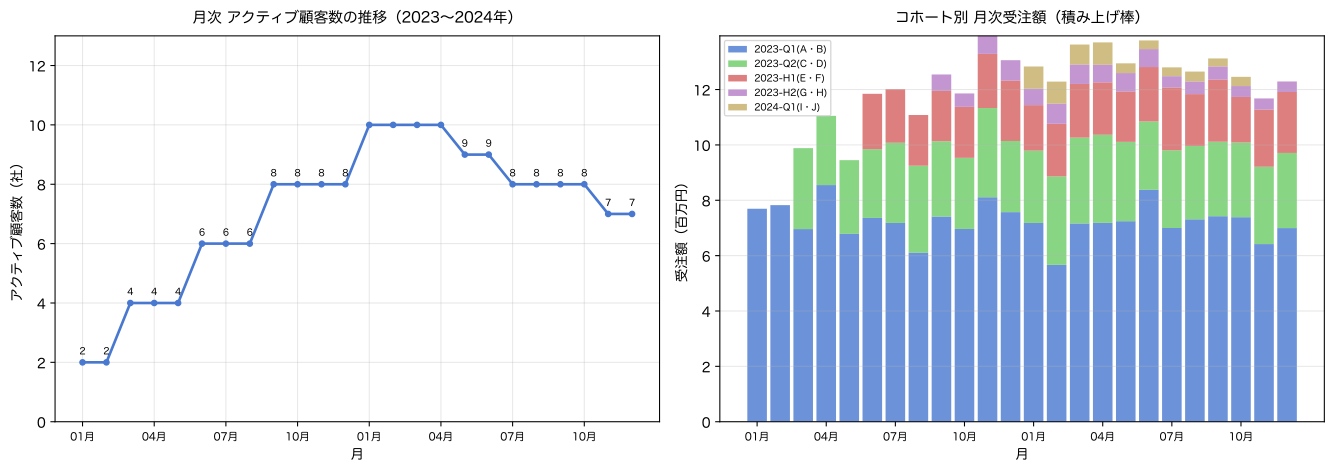

svg

データ概要グラフ表示完了（SVG 1/2）

No.081：コホート分析用のデータを作成する

実務での意味

コホート分析とは、共通の属性（例: 取引開始月）でグループ化し、グループごとの行動変化を時系列で追跡する分析手法です。

製造業での活用例：

OEM顧客の取引開始月別コホートで「何ヶ月目に解約が集中するか」を把握
製造設備の導入月別コホートで「稼働後 N ヶ月目の不良率変化」を追跡
品質改善プロジェクト開始月別で「改善効果が何ヶ月後に表れるか」を比較

分析・モデル化の考え方

コホート分析の基本構造は「誰が、いつ始めたか × 開始後 N ヶ月目の状態」です。

\text{month\_offset}_i = (\text{year}_i - \text{year}_0) \times 12 + (\text{month}_i - \text{month}_0)

$\text{month\_offset} = 0$ が取引開始月（コホート月）、 $= 1$ が翌月、 $= N$ が N ヶ月後を意味します。

SQLite では STRFTIME による日付演算より、文字列から年・月を取り出す SUBSTR + CAST の方が安定しています。

Python で確認する

# No.081: コホート基準テーブルの作成

print('=== customers マスタ（コホート月・解約月付き）===')
q(conn, '''
SELECT customer_id, customer_name, first_order_month,
       cancel_month, segment
FROM   customers
ORDER  BY first_order_month, customer_id
''')

print()
print('=== コホートデータ（customer_id × month × month_offset）===')
q(conn, '''
WITH cohort_base AS (
    SELECT customer_id, first_order_month AS cohort_month
    FROM   customers
),
cohort_data AS (
    SELECT o.customer_id,
           cb.cohort_month,
           o.month,
           (CAST(SUBSTR(o.month, 1, 4) AS INT)
            - CAST(SUBSTR(cb.cohort_month, 1, 4) AS INT)) * 12
           + CAST(SUBSTR(o.month, 6, 2) AS INT)
           - CAST(SUBSTR(cb.cohort_month, 6, 2) AS INT) AS month_offset
    FROM   orders o
    JOIN   cohort_base cb ON o.customer_id = cb.customer_id
)
SELECT cohort_month,
       month_offset,
       COUNT(DISTINCT customer_id) AS active_customers
FROM   cohort_data
GROUP  BY cohort_month, month_offset
ORDER  BY cohort_month, month_offset
LIMIT  20
''')

=== customers マスタ（コホート月・解約月付き）===
── SQL ─────────────────────────────────────────
  SELECT customer_id, customer_name, first_order_month,
         cancel_month, segment
  FROM   customers
  ORDER  BY first_order_month, customer_id
───────────────────────────────────────────────
shape: (10, 5)
┌─────────────┬───────────────┬───────────────────┬──────────────┬─────────┐
│ customer_id ┆ customer_name ┆ first_order_month ┆ cancel_month ┆ segment │
│ ---         ┆ ---           ┆ ---               ┆ ---          ┆ ---     │
│ str         ┆ str           ┆ str               ┆ str          ┆ str     │
╞═════════════╪═══════════════╪═══════════════════╪══════════════╪═════════╡
│ CUS-001     ┆ OEMメーカーA  ┆ 2023-01           ┆ null         ┆ 大手    │
│ CUS-002     ┆ OEMメーカーB  ┆ 2023-01           ┆ null         ┆ 大手    │
│ CUS-003     ┆ OEMメーカーC  ┆ 2023-03           ┆ null         ┆ 中堅    │
│ CUS-004     ┆ OEMメーカーD  ┆ 2023-03           ┆ null         ┆ 中堅    │
│ CUS-005     ┆ OEMメーカーE  ┆ 2023-06           ┆ null         ┆ 中堅    │
│ CUS-006     ┆ OEMメーカーF  ┆ 2023-06           ┆ null         ┆ 中堅    │
│ CUS-007     ┆ OEMメーカーG  ┆ 2023-09           ┆ null         ┆ 中小    │
│ CUS-008     ┆ OEMメーカーH  ┆ 2023-09           ┆ 2024-06      ┆ 中小    │
│ CUS-009     ┆ OEMメーカーI  ┆ 2024-01           ┆ 2024-04      ┆ 中小    │
│ CUS-010     ┆ OEMメーカーJ  ┆ 2024-01           ┆ 2024-10      ┆ 中小    │
└─────────────┴───────────────┴───────────────────┴──────────────┴─────────┘
↳ 10 行取得

=== コホートデータ（customer_id × month × month_offset）===
── SQL ─────────────────────────────────────────
  WITH cohort_base AS (
      SELECT customer_id, first_order_month AS cohort_month
      FROM   customers
  ),
  cohort_data AS (
      SELECT o.customer_id,
             cb.cohort_month,
             o.month,
             (CAST(SUBSTR(o.month, 1, 4) AS INT)
              - CAST(SUBSTR(cb.cohort_month, 1, 4) AS INT)) * 12
             + CAST(SUBSTR(o.month, 6, 2) AS INT)
             - CAST(SUBSTR(cb.cohort_month, 6, 2) AS INT) AS month_offset
      FROM   orders o
      JOIN   cohort_base cb ON o.customer_id = cb.customer_id
  )
  SELECT cohort_month,
         month_offset,
         COUNT(DISTINCT customer_id) AS active_customers
  FROM   cohort_data
  GROUP  BY cohort_month, month_offset
  ORDER  BY cohort_month, month_offset
  LIMIT  20
───────────────────────────────────────────────
shape: (20, 3)
┌──────────────┬──────────────┬──────────────────┐
│ cohort_month ┆ month_offset ┆ active_customers │
│ ---          ┆ ---          ┆ ---              │
│ str          ┆ i64          ┆ i64              │
╞══════════════╪══════════════╪══════════════════╡
│ 2023-01      ┆ 0            ┆ 2                │
│ 2023-01      ┆ 1            ┆ 2                │
│ 2023-01      ┆ 2            ┆ 2                │
│ 2023-01      ┆ 3            ┆ 2                │
│ 2023-01      ┆ 4            ┆ 2                │
│ …            ┆ …            ┆ …                │
│ 2023-01      ┆ 15           ┆ 2                │
│ 2023-01      ┆ 16           ┆ 2                │
│ 2023-01      ┆ 17           ┆ 2                │
│ 2023-01      ┆ 18           ┆ 2                │
│ 2023-01      ┆ 19           ┆ 2                │
└──────────────┴──────────────┴──────────────────┘
↳ 20 行取得

shape: (20, 3)

cohort_month	month_offset	active_customers
str	i64	i64
”2023-01”	0	2
”2023-01”	1	2
”2023-01”	2	2
”2023-01”	3	2
”2023-01”	4	2
…	…	…
“2023-01”	15	2
”2023-01”	16	2
”2023-01”	17	2
”2023-01”	18	2
”2023-01”	19	2

結果の読み取り

customers マスタに first_order_month（コホート月）と cancel_month（解約月）を持たせることで、コホート分析の基盤が整います
month_offset の計算は「年差 × 12 + 月差」の整数演算で求めます。 month_offset = 0 が取引開始月、= 6 が6ヶ月後です
コホート月ごとに active_customers を集計すると、各コホートが各 month_offset 時点で何社アクティブだったかが一覧化できます
2023-09 コホートは2社（OEMメーカーG・H）で始まりましたが、 H が月途中で解約するため後半の month_offset では1社になります

No.082：月別継続率を計算する

実務での意味

継続率（リテンション率）は「コホート開始時に比べて何 % の顧客が N ヶ月後も取引を継続しているか」を示す KPI です。

製造業での活用例：

OEM顧客の継続率が 60% を下回る月（離脱加速月）を特定して営業施策を強化
設備・工程の改善プログラムの継続率をモニタリングして定着効果を測定
新規取引先の初期 3〜6 ヶ月継続率を契約継続予測の入力変数として活用

分析・モデル化の考え方

継続率の定義：

\text{retention\_pct}(t) = \frac{\text{active\_customers}(t)}{\text{cohort\_size}} \times 100

$t = 0$ のとき継続率 = 100%（コホート開始時は全員アクティブ）。時間とともに減少し、解約が集中する $t$ で急落します。

この継続率テーブルはコホート別に作成し、コホートヒートマップとして可視化するのが一般的です。

Python で確認する

# No.082: コホート別 月次継続率の算出

print('=== コホート別 月次継続率（retention_pct）===')
q(conn, '''
WITH cohort_data AS (
    SELECT o.customer_id,
           c.first_order_month AS cohort_month,
           o.month,
           (CAST(SUBSTR(o.month, 1, 4) AS INT)
            - CAST(SUBSTR(c.first_order_month, 1, 4) AS INT)) * 12
           + CAST(SUBSTR(o.month, 6, 2) AS INT)
           - CAST(SUBSTR(c.first_order_month, 6, 2) AS INT) AS month_offset
    FROM   orders o
    JOIN   customers c ON o.customer_id = c.customer_id
),
cohort_size AS (
    SELECT first_order_month AS cohort_month,
           COUNT(*)          AS cohort_size
    FROM   customers
    GROUP  BY first_order_month
),
active_by_offset AS (
    SELECT cohort_month, month_offset,
           COUNT(DISTINCT customer_id) AS active_count
    FROM   cohort_data
    GROUP  BY cohort_month, month_offset
)
SELECT a.cohort_month,
       a.month_offset,
       a.active_count,
       cs.cohort_size,
       ROUND(a.active_count * 100.0 / cs.cohort_size, 1) AS retention_pct
FROM   active_by_offset a
JOIN   cohort_size cs ON a.cohort_month = cs.cohort_month
ORDER  BY a.cohort_month, a.month_offset
''')

=== コホート別 月次継続率（retention_pct）===
── SQL ─────────────────────────────────────────
  WITH cohort_data AS (
      SELECT o.customer_id,
             c.first_order_month AS cohort_month,
             o.month,
             (CAST(SUBSTR(o.month, 1, 4) AS INT)
              - CAST(SUBSTR(c.first_order_month, 1, 4) AS INT)) * 12
             + CAST(SUBSTR(o.month, 6, 2) AS INT)
             - CAST(SUBSTR(c.first_order_month, 6, 2) AS INT) AS month_offset
      FROM   orders o
      JOIN   customers c ON o.customer_id = c.customer_id
  ),
  cohort_size AS (
      SELECT first_order_month AS cohort_month,
             COUNT(*)          AS cohort_size
      FROM   customers
      GROUP  BY first_order_month
  ),
  active_by_offset AS (
      SELECT cohort_month, month_offset,
             COUNT(DISTINCT customer_id) AS active_count
      FROM   cohort_data
      GROUP  BY cohort_month, month_offset
  )
  SELECT a.cohort_month,
         a.month_offset,
         a.active_count,
         cs.cohort_size,
         ROUND(a.active_count * 100.0 / cs.cohort_size, 1) AS retention_pct
  FROM   active_by_offset a
  JOIN   cohort_size cs ON a.cohort_month = cs.cohort_month
  ORDER  BY a.cohort_month, a.month_offset
───────────────────────────────────────────────
shape: (91, 5)
┌──────────────┬──────────────┬──────────────┬─────────────┬───────────────┐
│ cohort_month ┆ month_offset ┆ active_count ┆ cohort_size ┆ retention_pct │
│ ---          ┆ ---          ┆ ---          ┆ ---         ┆ ---           │
│ str          ┆ i64          ┆ i64          ┆ i64         ┆ f64           │
╞══════════════╪══════════════╪══════════════╪═════════════╪═══════════════╡
│ 2023-01      ┆ 0            ┆ 2            ┆ 2           ┆ 100.0         │
│ 2023-01      ┆ 1            ┆ 2            ┆ 2           ┆ 100.0         │
│ 2023-01      ┆ 2            ┆ 2            ┆ 2           ┆ 100.0         │
│ 2023-01      ┆ 3            ┆ 2            ┆ 2           ┆ 100.0         │
│ 2023-01      ┆ 4            ┆ 2            ┆ 2           ┆ 100.0         │
│ …            ┆ …            ┆ …            ┆ …           ┆ …             │
│ 2024-01      ┆ 5            ┆ 1            ┆ 2           ┆ 50.0          │
│ 2024-01      ┆ 6            ┆ 1            ┆ 2           ┆ 50.0          │
│ 2024-01      ┆ 7            ┆ 1            ┆ 2           ┆ 50.0          │
│ 2024-01      ┆ 8            ┆ 1            ┆ 2           ┆ 50.0          │
│ 2024-01      ┆ 9            ┆ 1            ┆ 2           ┆ 50.0          │
└──────────────┴──────────────┴──────────────┴─────────────┴───────────────┘
↳ 91 行取得

shape: (91, 5)

cohort_month	month_offset	active_count	cohort_size	retention_pct
str	i64	i64	i64	f64
”2023-01”	0	2	2	100.0
”2023-01”	1	2	2	100.0
”2023-01”	2	2	2	100.0
”2023-01”	3	2	2	100.0
”2023-01”	4	2	2	100.0
…	…	…	…	…
“2024-01”	5	1	2	50.0
”2024-01”	6	1	2	50.0
”2024-01”	7	1	2	50.0
”2024-01”	8	1	2	50.0
”2024-01”	9	1	2	50.0

結果の読み取り

cohort_size はコホートに属する顧客数（取引開始月が同じ顧客数）です。例えば 2023-09 コホートは G と H の2社（cohort_size = 2）
retention_pct = 100.0 の月（month_offset = 0）は全員がアクティブな開始月です
2023-09 コホートは 9〜10 ヶ月目付近（OEMメーカーH が解約する 2024-06 相当）で retention_pct が 100.0% → 50.0% に急落します
2024-01 コホートは2社とも早期に解約するため、継続率が急速に低下します。このコホートへのオンボーディング施策の見直しが示唆されます

No.083：解約率を計算する

実務での意味

解約率（チャーンレート）は「アクティブな顧客のうち、その月に取引を停止した顧客の割合」を示します。

製造業での活用例：

月次解約率を KPI としてモニタリングし、営業部門が早期対応できる体制を構築
解約月に共通する「受注量の急減」「不良率の上昇」などの先行シグナルを特定
解約が集中する季節（年度末・決算期）を把握して事前の引き留め施策を立案

分析・モデル化の考え方

解約率の定義：

\text{churn\_rate}(t) = \frac{\text{churned}(t)}{\text{active\_at\_start}(t)} \times 100

LEAD(month, 1) で「次月に注文があるか」を確認し、次月注文がない & データ終端でない = そのコホートの最終注文月 = 解約月と判定します。

Python で確認する

# No.083: LEAD を使った月次解約率の算出

print('=== 解約顧客の最終注文月（LEAD で判定）===')
q(conn, '''
WITH monthly_orders_lead AS (
    SELECT customer_id, month,
           LEAD(month, 1) OVER (
               PARTITION BY customer_id
               ORDER BY month
           ) AS next_month
    FROM   orders
),
churned AS (
    SELECT customer_id,
           month AS churn_month
    FROM   monthly_orders_lead
    WHERE  next_month IS NULL
      AND  month < '2024-12'          -- データ末尾 (2024-12) は解約扱いしない
)
SELECT ch.customer_id,
       c.customer_name,
       c.first_order_month,
       c.cancel_month AS expected_cancel,
       ch.churn_month AS detected_churn
FROM   churned ch
JOIN   customers c ON ch.customer_id = c.customer_id
ORDER  BY ch.churn_month
''')

print()
print('=== 月次解約率（churned / active_at_month × 100）===')
q(conn, '''
WITH monthly_orders_lead AS (
    SELECT customer_id, month,
           LEAD(month, 1) OVER (PARTITION BY customer_id ORDER BY month) AS next_month
    FROM   orders
),
churned AS (
    SELECT month AS churn_month, COUNT(*) AS churned_count
    FROM   monthly_orders_lead
    WHERE  next_month IS NULL AND month < '2024-12'
    GROUP  BY month
),
monthly_active AS (
    SELECT month, COUNT(DISTINCT customer_id) AS active_count
    FROM   orders
    GROUP  BY month
)
SELECT ma.month,
       ma.active_count,
       COALESCE(ch.churned_count, 0) AS churned,
       ROUND(COALESCE(ch.churned_count, 0) * 100.0 / ma.active_count, 1) AS churn_rate_pct
FROM   monthly_active ma
LEFT JOIN churned ch ON ma.month = ch.churn_month
ORDER  BY ma.month
''')

=== 解約顧客の最終注文月（LEAD で判定）===
── SQL ─────────────────────────────────────────
  WITH monthly_orders_lead AS (
      SELECT customer_id, month,
             LEAD(month, 1) OVER (
                 PARTITION BY customer_id
                 ORDER BY month
             ) AS next_month
      FROM   orders
  ),
  churned AS (
      SELECT customer_id,
             month AS churn_month
      FROM   monthly_orders_lead
      WHERE  next_month IS NULL
        AND  month < '2024-12'          -- データ末尾 (2024-12) は解約扱いしない
  )
  SELECT ch.customer_id,
         c.customer_name,
         c.first_order_month,
         c.cancel_month AS expected_cancel,
         ch.churn_month AS detected_churn
  FROM   churned ch
  JOIN   customers c ON ch.customer_id = c.customer_id
  ORDER  BY ch.churn_month
───────────────────────────────────────────────
shape: (3, 5)
┌─────────────┬───────────────┬───────────────────┬─────────────────┬────────────────┐
│ customer_id ┆ customer_name ┆ first_order_month ┆ expected_cancel ┆ detected_churn │
│ ---         ┆ ---           ┆ ---               ┆ ---             ┆ ---            │
│ str         ┆ str           ┆ str               ┆ str             ┆ str            │
╞═════════════╪═══════════════╪═══════════════════╪═════════════════╪════════════════╡
│ CUS-009     ┆ OEMメーカーI  ┆ 2024-01           ┆ 2024-04         ┆ 2024-04        │
│ CUS-008     ┆ OEMメーカーH  ┆ 2023-09           ┆ 2024-06         ┆ 2024-06        │
│ CUS-010     ┆ OEMメーカーJ  ┆ 2024-01           ┆ 2024-10         ┆ 2024-10        │
└─────────────┴───────────────┴───────────────────┴─────────────────┴────────────────┘
↳ 3 行取得

=== 月次解約率（churned / active_at_month × 100）===
── SQL ─────────────────────────────────────────
  WITH monthly_orders_lead AS (
      SELECT customer_id, month,
             LEAD(month, 1) OVER (PARTITION BY customer_id ORDER BY month) AS next_month
      FROM   orders
  ),
  churned AS (
      SELECT month AS churn_month, COUNT(*) AS churned_count
      FROM   monthly_orders_lead
      WHERE  next_month IS NULL AND month < '2024-12'
      GROUP  BY month
  ),
  monthly_active AS (
      SELECT month, COUNT(DISTINCT customer_id) AS active_count
      FROM   orders
      GROUP  BY month
  )
  SELECT ma.month,
         ma.active_count,
         COALESCE(ch.churned_count, 0) AS churned,
         ROUND(COALESCE(ch.churned_count, 0) * 100.0 / ma.active_count, 1) AS churn_rate_pct
  FROM   monthly_active ma
  LEFT JOIN churned ch ON ma.month = ch.churn_month
  ORDER  BY ma.month
───────────────────────────────────────────────
shape: (24, 4)
┌─────────┬──────────────┬─────────┬────────────────┐
│ month   ┆ active_count ┆ churned ┆ churn_rate_pct │
│ ---     ┆ ---          ┆ ---     ┆ ---            │
│ str     ┆ i64          ┆ i64     ┆ f64            │
╞═════════╪══════════════╪═════════╪════════════════╡
│ 2023-01 ┆ 2            ┆ 0       ┆ 0.0            │
│ 2023-02 ┆ 2            ┆ 0       ┆ 0.0            │
│ 2023-03 ┆ 4            ┆ 0       ┆ 0.0            │
│ 2023-04 ┆ 4            ┆ 0       ┆ 0.0            │
│ 2023-05 ┆ 4            ┆ 0       ┆ 0.0            │
│ …       ┆ …            ┆ …       ┆ …              │
│ 2024-08 ┆ 8            ┆ 0       ┆ 0.0            │
│ 2024-09 ┆ 8            ┆ 0       ┆ 0.0            │
│ 2024-10 ┆ 8            ┆ 1       ┆ 12.5           │
│ 2024-11 ┆ 7            ┆ 0       ┆ 0.0            │
│ 2024-12 ┆ 7            ┆ 0       ┆ 0.0            │
└─────────┴──────────────┴─────────┴────────────────┘
↳ 24 行取得

shape: (24, 4)

month	active_count	churned	churn_rate_pct
str	i64	i64	f64
”2023-01”	2	0	0.0
”2023-02”	2	0	0.0
”2023-03”	4	0	0.0
”2023-04”	4	0	0.0
”2023-05”	4	0	0.0
…	…	…	…
“2024-08”	8	0	0.0
”2024-09”	8	0	0.0
”2024-10”	8	1	12.5
”2024-11”	7	0	0.0
”2024-12”	7	0	0.0

結果の読み取り

LEAD(month, 1) が NULL となる行は「その顧客の最後の注文月」です。 month < '2024-12' 条件でデータ末尾を除外することで、真の解約のみを検出できます
detected_churn と expected_cancel（cancel_month）が一致していることで、 LEAD による解約判定の正確性が確認できます
月次解約率は通常 0〜1 件/月程度の水準でも推移しますが、解約が集中した月（例: 2024-04、2024-06、2024-10）が可視化されます
解約率が突発的に上昇した月の「前月・前々月の受注量トレンド」を調べることで、解約の先行シグナルを特定できます

No.084：ファネル分析用のデータを作成する

実務での意味

ファネル分析は「ある目標に向けたプロセスの各段階で、どれだけが次段階に進めるか」を可視化する分析手法です。

製造業での活用例：

製造ファネル（投入 → 一次検査合格 → 二次検査合格 → 出荷）の各段階の歩留まり把握
「どの工程で最も多く品質ロスが発生しているか」を定量化して改善優先度を設定
複数ラインのファネルを比較して工程設計・設備能力の差異を可視化

分析・モデル化の考え方

製造ファネルの各段階の歩留まりと総合歩留まり：

Y_{\text{overall}} = Y_1 \times Y_2 \times Y_3

Y_1 = \frac{\text{一次検査合格}}{\text{投入}},\; Y_2 = \frac{\text{二次検査合格}}{\text{一次検査合格}},\; Y_3 = \frac{\text{出荷}}{\text{二次検査合格}}

各段階の歩留まりが分かると「ボトルネック工程」が特定でき、改善投資の効果を最大化できます。

Python で確認する

# No.084: 製造ファネルデータの作成と各段階の歩留まり算出

print('=== ライン別 製造工程ファネル（年間集計）===')
q(conn, '''
SELECT line_code,
       SUM(input_qty)       AS stage0_input,
       SUM(first_pass_qty)  AS stage1_first_check,
       SUM(second_pass_qty) AS stage2_second_check,
       SUM(shipped_qty)     AS stage3_shipped
FROM   lot_records
GROUP  BY line_code
ORDER  BY line_code
''')

print()
print('=== 各工程の歩留まり率（%）と総合歩留まり ===')
q(conn, '''
WITH funnel AS (
    SELECT line_code,
           SUM(input_qty)       AS s0,
           SUM(first_pass_qty)  AS s1,
           SUM(second_pass_qty) AS s2,
           SUM(shipped_qty)     AS s3
    FROM   lot_records
    GROUP  BY line_code
)
SELECT line_code,
       s0 AS input_qty,
       s3 AS shipped_qty,
       ROUND(s1 * 100.0 / s0, 2) AS first_pass_pct,
       ROUND(s2 * 100.0 / s1, 2) AS second_pass_pct,
       ROUND(s3 * 100.0 / s2, 2) AS ship_pct,
       ROUND(s3 * 100.0 / s0, 2) AS overall_yield_pct,
       s0 - s3                   AS total_loss_qty
FROM   funnel
ORDER  BY overall_yield_pct
''')

=== ライン別 製造工程ファネル（年間集計）===
── SQL ─────────────────────────────────────────
  SELECT line_code,
         SUM(input_qty)       AS stage0_input,
         SUM(first_pass_qty)  AS stage1_first_check,
         SUM(second_pass_qty) AS stage2_second_check,
         SUM(shipped_qty)     AS stage3_shipped
  FROM   lot_records
  GROUP  BY line_code
  ORDER  BY line_code
───────────────────────────────────────────────
shape: (5, 5)
┌───────────┬──────────────┬────────────────────┬─────────────────────┬────────────────┐
│ line_code ┆ stage0_input ┆ stage1_first_check ┆ stage2_second_check ┆ stage3_shipped │
│ ---       ┆ ---          ┆ ---                ┆ ---                 ┆ ---            │
│ str       ┆ i64          ┆ i64                ┆ i64                 ┆ i64            │
╞═══════════╪══════════════╪════════════════════╪═════════════════════╪════════════════╡
│ LINE-A1   ┆ 42905        ┆ 41414              ┆ 40742               ┆ 40622          │
│ LINE-A2   ┆ 33783        ┆ 32370              ┆ 31676               ┆ 31605          │
│ LINE-B1   ┆ 41133        ┆ 39516              ┆ 38753               ┆ 38633          │
│ LINE-C1   ┆ 15530        ┆ 14647              ┆ 14303               ┆ 14252          │
│ LINE-D1   ┆ 35768        ┆ 34382              ┆ 33771               ┆ 33699          │
└───────────┴──────────────┴────────────────────┴─────────────────────┴────────────────┘
↳ 5 行取得

=== 各工程の歩留まり率（%）と総合歩留まり ===
── SQL ─────────────────────────────────────────
  WITH funnel AS (
      SELECT line_code,
             SUM(input_qty)       AS s0,
             SUM(first_pass_qty)  AS s1,
             SUM(second_pass_qty) AS s2,
             SUM(shipped_qty)     AS s3
      FROM   lot_records
      GROUP  BY line_code
  )
  SELECT line_code,
         s0 AS input_qty,
         s3 AS shipped_qty,
         ROUND(s1 * 100.0 / s0, 2) AS first_pass_pct,
         ROUND(s2 * 100.0 / s1, 2) AS second_pass_pct,
         ROUND(s3 * 100.0 / s2, 2) AS ship_pct,
         ROUND(s3 * 100.0 / s0, 2) AS overall_yield_pct,
         s0 - s3                   AS total_loss_qty
  FROM   funnel
  ORDER  BY overall_yield_pct
───────────────────────────────────────────────
shape: (5, 8)
┌───────────┬───────────┬────────────┬────────────┬────────────┬──────────┬────────────┬───────────┐
│ line_code ┆ input_qty ┆ shipped_qt ┆ first_pass ┆ second_pas ┆ ship_pct ┆ overall_yi ┆ total_los │
│ ---       ┆ ---       ┆ y          ┆ _pct       ┆ s_pct      ┆ ---      ┆ eld_pct    ┆ s_qty     │
│ str       ┆ i64       ┆ ---        ┆ ---        ┆ ---        ┆ f64      ┆ ---        ┆ ---       │
│           ┆           ┆ i64        ┆ f64        ┆ f64        ┆          ┆ f64        ┆ i64       │
╞═══════════╪═══════════╪════════════╪════════════╪════════════╪══════════╪════════════╪═══════════╡
│ LINE-C1   ┆ 15530     ┆ 14252      ┆ 94.31      ┆ 97.65      ┆ 99.64    ┆ 91.77      ┆ 1278      │
│ LINE-A2   ┆ 33783     ┆ 31605      ┆ 95.82      ┆ 97.86      ┆ 99.78    ┆ 93.55      ┆ 2178      │
│ LINE-B1   ┆ 41133     ┆ 38633      ┆ 96.07      ┆ 98.07      ┆ 99.69    ┆ 93.92      ┆ 2500      │
│ LINE-D1   ┆ 35768     ┆ 33699      ┆ 96.13      ┆ 98.22      ┆ 99.79    ┆ 94.22      ┆ 2069      │
│ LINE-A1   ┆ 42905     ┆ 40622      ┆ 96.52      ┆ 98.38      ┆ 99.71    ┆ 94.68      ┆ 2283      │
└───────────┴───────────┴────────────┴────────────┴────────────┴──────────┴────────────┴───────────┘
↳ 5 行取得

shape: (5, 8)

line_code	input_qty	shipped_qty	first_pass_pct	second_pass_pct	ship_pct	overall_yield_pct	total_loss_qty
str	i64	i64	f64	f64	f64	f64	i64
”LINE-C1”	15530	14252	94.31	97.65	99.64	91.77	1278
”LINE-A2”	33783	31605	95.82	97.86	99.78	93.55	2178
”LINE-B1”	41133	38633	96.07	98.07	99.69	93.92	2500
”LINE-D1”	35768	33699	96.13	98.22	99.79	94.22	2069
”LINE-A1”	42905	40622	96.52	98.38	99.71	94.68	2283

結果の読み取り

first_pass_pct（一次検査合格率）が最も低いライン（LINE-C1）が製造ファネルのボトルネック工程です。ここへの投資が総合歩留まりの改善に直結します
overall_yield_pct（総合歩留まり）は各工程歩留まりの積です。例えば 96.5% × 98.2% × 99.7% = 94.5% 程度になります
total_loss_qty（廃棄・手直し数量）に単価を掛けると「品質損失コスト」が算出できます。LINE-C1 は件数が少なくても損失コストが相対的に高い可能性があります
ファネル分析は月次で集計することで「歩留まりの月次変動」も監視できます

No.085：ユーザー行動ログを集計する

実務での意味

設備イベントログ（アラーム・警告・緊急停止などのイベント記録）を集計することで、設備の稼働状態と異常発生傾向を定量的に把握できます。

製造業での活用例：

ライン別・月別のアラーム件数を集計して「アラームが多いライン」を優先保全
ロット単位のアラーム密度（アラーム/ロット）を KPI として管理
アラーム件数が突発増加した月の製造記録を精査して原因を特定

分析・モデル化の考え方

アラーム密度の定義：

\text{alarm\_density} = \frac{\sum \text{alarm\_count}}{\text{lot\_count}}

設備の正常稼働時のアラーム密度は低く（例: 1 件/ロット未満）、予防保全タイミングの接近・設備劣化・工程異常時に上昇します。 alarm_density のトレンドを追跡することで予防保全の判断指標として使えます。

Python で確認する

# No.085: 設備イベントログの集計（アラーム件数 / アラーム密度）

print('=== ライン別 年間アラーム件数と密度 ===')
q(conn, '''
SELECT line_code,
       COUNT(lot_id)                                       AS lot_count,
       SUM(alarm_count)                                    AS total_alarms,
       ROUND(SUM(alarm_count) * 1.0 / COUNT(lot_id), 2)  AS alarm_density,
       MAX(alarm_count)                                    AS max_alarms_per_lot,
       SUM(CASE WHEN alarm_count = 0 THEN 1 ELSE 0 END)   AS zero_alarm_lots
FROM   lot_records
GROUP  BY line_code
ORDER  BY total_alarms DESC
''')

print()
print('=== 月次 アラーム件数ランキング（全ライン、上位12件）===')
q(conn, '''
SELECT month, line_code,
       SUM(alarm_count)  AS monthly_alarms,
       COUNT(lot_id)     AS lots,
       ROUND(SUM(alarm_count) * 1.0 / COUNT(lot_id), 1) AS density
FROM   lot_records
WHERE  alarm_count > 0
GROUP  BY month, line_code
ORDER  BY monthly_alarms DESC
LIMIT  12
''')

=== ライン別 年間アラーム件数と密度 ===
── SQL ─────────────────────────────────────────
  SELECT line_code,
         COUNT(lot_id)                                       AS lot_count,
         SUM(alarm_count)                                    AS total_alarms,
         ROUND(SUM(alarm_count) * 1.0 / COUNT(lot_id), 2)  AS alarm_density,
         MAX(alarm_count)                                    AS max_alarms_per_lot,
         SUM(CASE WHEN alarm_count = 0 THEN 1 ELSE 0 END)   AS zero_alarm_lots
  FROM   lot_records
  GROUP  BY line_code
  ORDER  BY total_alarms DESC
───────────────────────────────────────────────
shape: (5, 6)
┌───────────┬───────────┬──────────────┬───────────────┬────────────────────┬─────────────────┐
│ line_code ┆ lot_count ┆ total_alarms ┆ alarm_density ┆ max_alarms_per_lot ┆ zero_alarm_lots │
│ ---       ┆ ---       ┆ ---          ┆ ---           ┆ ---                ┆ ---             │
│ str       ┆ i64       ┆ i64          ┆ f64           ┆ i64                ┆ i64             │
╞═══════════╪═══════════╪══════════════╪═══════════════╪════════════════════╪═════════════════╡
│ LINE-B1   ┆ 24        ┆ 34           ┆ 1.42          ┆ 5                  ┆ 8               │
│ LINE-D1   ┆ 24        ┆ 26           ┆ 1.08          ┆ 3                  ┆ 11              │
│ LINE-A2   ┆ 24        ┆ 26           ┆ 1.08          ┆ 3                  ┆ 8               │
│ LINE-C1   ┆ 24        ┆ 25           ┆ 1.04          ┆ 2                  ┆ 7               │
│ LINE-A1   ┆ 24        ┆ 23           ┆ 0.96          ┆ 4                  ┆ 11              │
└───────────┴───────────┴──────────────┴───────────────┴────────────────────┴─────────────────┘
↳ 5 行取得

=== 月次 アラーム件数ランキング（全ライン、上位12件）===
── SQL ─────────────────────────────────────────
  SELECT month, line_code,
         SUM(alarm_count)  AS monthly_alarms,
         COUNT(lot_id)     AS lots,
         ROUND(SUM(alarm_count) * 1.0 / COUNT(lot_id), 1) AS density
  FROM   lot_records
  WHERE  alarm_count > 0
  GROUP  BY month, line_code
  ORDER  BY monthly_alarms DESC
  LIMIT  12
───────────────────────────────────────────────
shape: (12, 5)
┌─────────┬───────────┬────────────────┬──────┬─────────┐
│ month   ┆ line_code ┆ monthly_alarms ┆ lots ┆ density │
│ ---     ┆ ---       ┆ ---            ┆ ---  ┆ ---     │
│ str     ┆ str       ┆ i64            ┆ i64  ┆ f64     │
╞═════════╪═══════════╪════════════════╪══════╪═════════╡
│ 2024-03 ┆ LINE-D1   ┆ 6              ┆ 2    ┆ 3.0     │
│ 2024-06 ┆ LINE-B1   ┆ 6              ┆ 2    ┆ 3.0     │
│ 2024-02 ┆ LINE-B1   ┆ 5              ┆ 1    ┆ 5.0     │
│ 2024-04 ┆ LINE-A2   ┆ 5              ┆ 2    ┆ 2.5     │
│ 2024-04 ┆ LINE-B1   ┆ 5              ┆ 2    ┆ 2.5     │
│ …       ┆ …         ┆ …              ┆ …    ┆ …       │
│ 2024-06 ┆ LINE-A2   ┆ 4              ┆ 2    ┆ 2.0     │
│ 2024-09 ┆ LINE-B1   ┆ 4              ┆ 2    ┆ 2.0     │
│ 2024-09 ┆ LINE-C1   ┆ 4              ┆ 2    ┆ 2.0     │
│ 2024-11 ┆ LINE-B1   ┆ 4              ┆ 2    ┆ 2.0     │
│ 2024-11 ┆ LINE-C1   ┆ 4              ┆ 2    ┆ 2.0     │
└─────────┴───────────┴────────────────┴──────┴─────────┘
↳ 12 行取得

shape: (12, 5)

month	line_code	monthly_alarms	lots	density
str	str	i64	i64	f64
”2024-03"	"LINE-D1”	6	2	3.0
”2024-06"	"LINE-B1”	6	2	3.0
”2024-02"	"LINE-B1”	5	1	5.0
”2024-04"	"LINE-A2”	5	2	2.5
”2024-04"	"LINE-B1”	5	2	2.5
…	…	…	…	…
“2024-06"	"LINE-A2”	4	2	2.0
”2024-09"	"LINE-B1”	4	2	2.0
”2024-09"	"LINE-C1”	4	2	2.0
”2024-11"	"LINE-B1”	4	2	2.0
”2024-11"	"LINE-C1”	4	2	2.0

結果の読み取り

total_alarms が多いラインは「累積アラーム件数の大きいライン」ですが、 lot_count も多いラインほど自然にアラーム件数が増えます。 アラーム密度（alarm_density）で正規化することが重要です
max_alarms_per_lot が 3 以上のロットが存在する場合は、そのロットが実施された日時の設備状態を詳細調査する価値があります
zero_alarm_lots（アラームゼロのロット数）が多いラインほど安定稼働しています。改善活動の目標として「zero_alarm_lots 比率 N% 以上」を設定できます
月次集計のランキングで「特定の月に特定ラインのアラームが集中」していれば、その月に何が起きたかの原因調査の起点になります

No.086：セッション数を集計する

実務での意味

生産セッション（バッチ）は「一つの製造ロットを生産するための設備稼働単位」です。セッション数と稼働時間の集計により、設備の利用効率が把握できます。

製造業での活用例：

ライン別の月次セッション数と稼働時間を集計して稼働率を計算
平均セッション時間（avg_session_minutes）の変化をモニタリングして段取り・手直し・待機時間の増加を検出
計画稼働時間に対して実績セッション時間が乖離する月を特定

分析・モデル化の考え方

設備稼働率（可用率）の定義：

\text{稼働率} = \frac{\sum \text{session\_minutes}}{\text{計画稼働時間（分）}} \times 100

1ヶ月の計画稼働時間を 8時間/日 × 22日 = 10,560 分と仮定すると、月次セッション合計時間との比較で稼働率が算出できます。

Python で確認する

# No.086: 生産セッション数と稼働時間の集計

PLANNED_MINUTES_MONTH = 8 * 60 * 22  # 8h × 22日 = 10,560分

print('=== ライン別 年間セッション集計 ===')
q(conn, '''
SELECT line_code,
       COUNT(lot_id)                         AS total_sessions,
       SUM(session_minutes)                  AS total_minutes,
       ROUND(AVG(session_minutes), 1)        AS avg_session_min,
       MIN(session_minutes)                  AS min_session_min,
       MAX(session_minutes)                  AS max_session_min
FROM   lot_records
GROUP  BY line_code
ORDER  BY total_sessions DESC
''')

print()
print('=== 月次 セッション数 × 稼働時間（全ライン合計）===')
q(conn, '''
SELECT month,
       COUNT(lot_id)              AS monthly_sessions,
       SUM(session_minutes)       AS total_minutes,
       ROUND(AVG(session_minutes), 1) AS avg_minutes
FROM   lot_records
GROUP  BY month
ORDER  BY month
''')

print()
print(f'参考: 1ライン計画稼働時間 = {PLANNED_MINUTES_MONTH:,} 分/月（8h×22日）')

=== ライン別 年間セッション集計 ===
── SQL ─────────────────────────────────────────
  SELECT line_code,
         COUNT(lot_id)                         AS total_sessions,
         SUM(session_minutes)                  AS total_minutes,
         ROUND(AVG(session_minutes), 1)        AS avg_session_min,
         MIN(session_minutes)                  AS min_session_min,
         MAX(session_minutes)                  AS max_session_min
  FROM   lot_records
  GROUP  BY line_code
  ORDER  BY total_sessions DESC
───────────────────────────────────────────────
shape: (5, 6)
┌───────────┬────────────────┬───────────────┬─────────────────┬─────────────────┬─────────────────┐
│ line_code ┆ total_sessions ┆ total_minutes ┆ avg_session_min ┆ min_session_min ┆ max_session_min │
│ ---       ┆ ---            ┆ ---           ┆ ---             ┆ ---             ┆ ---             │
│ str       ┆ i64            ┆ i64           ┆ f64             ┆ i64             ┆ i64             │
╞═══════════╪════════════════╪═══════════════╪═════════════════╪═════════════════╪═════════════════╡
│ LINE-D1   ┆ 24             ┆ 6624          ┆ 276.0           ┆ 235             ┆ 324             │
│ LINE-C1   ┆ 24             ┆ 6794          ┆ 283.1           ┆ 186             ┆ 346             │
│ LINE-B1   ┆ 24             ┆ 6499          ┆ 270.8           ┆ 216             ┆ 344             │
│ LINE-A2   ┆ 24             ┆ 6607          ┆ 275.3           ┆ 216             ┆ 316             │
│ LINE-A1   ┆ 24             ┆ 7016          ┆ 292.3           ┆ 198             ┆ 375             │
└───────────┴────────────────┴───────────────┴─────────────────┴─────────────────┴─────────────────┘
↳ 5 行取得

=== 月次 セッション数 × 稼働時間（全ライン合計）===
── SQL ─────────────────────────────────────────
  SELECT month,
         COUNT(lot_id)              AS monthly_sessions,
         SUM(session_minutes)       AS total_minutes,
         ROUND(AVG(session_minutes), 1) AS avg_minutes
  FROM   lot_records
  GROUP  BY month
  ORDER  BY month
───────────────────────────────────────────────
shape: (12, 4)
┌─────────┬──────────────────┬───────────────┬─────────────┐
│ month   ┆ monthly_sessions ┆ total_minutes ┆ avg_minutes │
│ ---     ┆ ---              ┆ ---           ┆ ---         │
│ str     ┆ i64              ┆ i64           ┆ f64         │
╞═════════╪══════════════════╪═══════════════╪═════════════╡
│ 2024-01 ┆ 10               ┆ 2906          ┆ 290.6       │
│ 2024-02 ┆ 10               ┆ 2899          ┆ 289.9       │
│ 2024-03 ┆ 10               ┆ 2837          ┆ 283.7       │
│ 2024-04 ┆ 10               ┆ 2896          ┆ 289.6       │
│ 2024-05 ┆ 10               ┆ 2813          ┆ 281.3       │
│ …       ┆ …                ┆ …             ┆ …           │
│ 2024-08 ┆ 10               ┆ 2643          ┆ 264.3       │
│ 2024-09 ┆ 10               ┆ 2853          ┆ 285.3       │
│ 2024-10 ┆ 10               ┆ 2641          ┆ 264.1       │
│ 2024-11 ┆ 10               ┆ 2764          ┆ 276.4       │
│ 2024-12 ┆ 10               ┆ 2636          ┆ 263.6       │
└─────────┴──────────────────┴───────────────┴─────────────┘
↳ 12 行取得

参考: 1ライン計画稼働時間 = 10,560 分/月（8h×22日）

結果の読み取り

total_sessions（月次: 全ライン合計24 = 5ライン × 2バッチ × 12ヶ月 / 12）は各月で一定です（月2バッチ設計）。実際の現場では計画外停止で変動します
avg_session_min（平均セッション時間）の変化をトレンド追跡します。増加傾向は「段取り時間の悪化」「設備劣化による速度低下」などのシグナルです
total_minutes を計画稼働時間（1ライン 10,560分/月）で割ると稼働率が算出できます。ラインごとの月次稼働率 KPI として経営会議に報告できます
セッション数が少ない月（計画停止・連休等）と多い月（残業・休日出勤等）の差異分析は、コスト・品質の季節変動理解に役立ちます

No.087：コンバージョン率を計算する

実務での意味

製造業におけるコンバージョン率は「投入した原材料・仕掛品がどれだけ良品として出荷されるか」を示す総合歩留まり率です。

製造業での活用例：

ライン別の年間・月次総合歩留まりを算出して原価計算の基礎データにする
総合歩留まりの改善量を金額換算して改善投資の ROI を算出
各工程の歩留まりを比較して「どの工程の改善が最も効果的か」を定量化

分析・モデル化の考え方

ファネルの全体コンバージョン率（総合歩留まり）：

\text{overall\_yield\_pct} = \frac{\text{出荷数}}{\text{投入数}} \times 100 \;=\; Y_1 \times Y_2 \times Y_3 \times 100

品質コスト（廃棄・手直しコスト）は：

\text{quality\_loss} = (\text{投入数} - \text{出荷数}) \times \text{単価}

この品質ロスコストが最大のラインへの改善投資が ROI 最大化につながります。

Python で確認する

# No.087: 製造歩留まり率（コンバージョン率）の算出

print('=== ライン別 総合歩留まり率と各工程ブレークダウン ===')
q(conn, '''
WITH funnel AS (
    SELECT lr.line_code,
           SUM(lr.input_qty)         AS s0,
           SUM(lr.first_pass_qty)    AS s1,
           SUM(lr.second_pass_qty)   AS s2,
           SUM(lr.shipped_qty)       AS s3
    FROM   lot_records lr
    GROUP  BY lr.line_code
)
SELECT f.line_code,
       f.s0                             AS input_qty,
       f.s3                             AS shipped_qty,
       f.s0 - f.s3                      AS loss_qty,
       ROUND(f.s1 * 100.0 / f.s0, 2)   AS first_pass_pct,
       ROUND(f.s2 * 100.0 / f.s1, 2)   AS second_pass_pct,
       ROUND(f.s3 * 100.0 / f.s2, 2)   AS ship_pct,
       ROUND(f.s3 * 100.0 / f.s0, 2)   AS overall_yield_pct
FROM   funnel f
ORDER  BY overall_yield_pct
''')

print()
print('=== 月次 全体の平均歩留まり率（全ライン合計）===')
q(conn, '''
SELECT month,
       SUM(input_qty)  AS monthly_input,
       SUM(shipped_qty) AS monthly_shipped,
       ROUND(SUM(shipped_qty) * 100.0 / SUM(input_qty), 2) AS monthly_yield_pct
FROM   lot_records
GROUP  BY month
ORDER  BY month
''')

=== ライン別 総合歩留まり率と各工程ブレークダウン ===
── SQL ─────────────────────────────────────────
  WITH funnel AS (
      SELECT lr.line_code,
             SUM(lr.input_qty)         AS s0,
             SUM(lr.first_pass_qty)    AS s1,
             SUM(lr.second_pass_qty)   AS s2,
             SUM(lr.shipped_qty)       AS s3
      FROM   lot_records lr
      GROUP  BY lr.line_code
  )
  SELECT f.line_code,
         f.s0                             AS input_qty,
         f.s3                             AS shipped_qty,
         f.s0 - f.s3                      AS loss_qty,
         ROUND(f.s1 * 100.0 / f.s0, 2)   AS first_pass_pct,
         ROUND(f.s2 * 100.0 / f.s1, 2)   AS second_pass_pct,
         ROUND(f.s3 * 100.0 / f.s2, 2)   AS ship_pct,
         ROUND(f.s3 * 100.0 / f.s0, 2)   AS overall_yield_pct
  FROM   funnel f
  ORDER  BY overall_yield_pct
───────────────────────────────────────────────
shape: (5, 8)
┌───────────┬───────────┬─────────────┬──────────┬────────────┬────────────┬──────────┬────────────┐
│ line_code ┆ input_qty ┆ shipped_qty ┆ loss_qty ┆ first_pass ┆ second_pas ┆ ship_pct ┆ overall_yi │
│ ---       ┆ ---       ┆ ---         ┆ ---      ┆ _pct       ┆ s_pct      ┆ ---      ┆ eld_pct    │
│ str       ┆ i64       ┆ i64         ┆ i64      ┆ ---        ┆ ---        ┆ f64      ┆ ---        │
│           ┆           ┆             ┆          ┆ f64        ┆ f64        ┆          ┆ f64        │
╞═══════════╪═══════════╪═════════════╪══════════╪════════════╪════════════╪══════════╪════════════╡
│ LINE-C1   ┆ 15530     ┆ 14252       ┆ 1278     ┆ 94.31      ┆ 97.65      ┆ 99.64    ┆ 91.77      │
│ LINE-A2   ┆ 33783     ┆ 31605       ┆ 2178     ┆ 95.82      ┆ 97.86      ┆ 99.78    ┆ 93.55      │
│ LINE-B1   ┆ 41133     ┆ 38633       ┆ 2500     ┆ 96.07      ┆ 98.07      ┆ 99.69    ┆ 93.92      │
│ LINE-D1   ┆ 35768     ┆ 33699       ┆ 2069     ┆ 96.13      ┆ 98.22      ┆ 99.79    ┆ 94.22      │
│ LINE-A1   ┆ 42905     ┆ 40622       ┆ 2283     ┆ 96.52      ┆ 98.38      ┆ 99.71    ┆ 94.68      │
└───────────┴───────────┴─────────────┴──────────┴────────────┴────────────┴──────────┴────────────┘
↳ 5 行取得

=== 月次 全体の平均歩留まり率（全ライン合計）===
── SQL ─────────────────────────────────────────
  SELECT month,
         SUM(input_qty)  AS monthly_input,
         SUM(shipped_qty) AS monthly_shipped,
         ROUND(SUM(shipped_qty) * 100.0 / SUM(input_qty), 2) AS monthly_yield_pct
  FROM   lot_records
  GROUP  BY month
  ORDER  BY month
───────────────────────────────────────────────
shape: (12, 4)
┌─────────┬───────────────┬─────────────────┬───────────────────┐
│ month   ┆ monthly_input ┆ monthly_shipped ┆ monthly_yield_pct │
│ ---     ┆ ---           ┆ ---             ┆ ---               │
│ str     ┆ i64           ┆ i64             ┆ f64               │
╞═════════╪═══════════════╪═════════════════╪═══════════════════╡
│ 2024-01 ┆ 14179         ┆ 13276           ┆ 93.63             │
│ 2024-02 ┆ 14121         ┆ 13230           ┆ 93.69             │
│ 2024-03 ┆ 13823         ┆ 13020           ┆ 94.19             │
│ 2024-04 ┆ 14278         ┆ 13411           ┆ 93.93             │
│ 2024-05 ┆ 13947         ┆ 13153           ┆ 94.31             │
│ …       ┆ …             ┆ …               ┆ …                 │
│ 2024-08 ┆ 14049         ┆ 13261           ┆ 94.39             │
│ 2024-09 ┆ 14037         ┆ 13067           ┆ 93.09             │
│ 2024-10 ┆ 14368         ┆ 13452           ┆ 93.62             │
│ 2024-11 ┆ 14347         ┆ 13506           ┆ 94.14             │
│ 2024-12 ┆ 14016         ┆ 13176           ┆ 94.01             │
└─────────┴───────────────┴─────────────────┴───────────────────┘
↳ 12 行取得

shape: (12, 4)

month	monthly_input	monthly_shipped	monthly_yield_pct
str	i64	i64	f64
”2024-01”	14179	13276	93.63
”2024-02”	14121	13230	93.69
”2024-03”	13823	13020	94.19
”2024-04”	14278	13411	93.93
”2024-05”	13947	13153	94.31
…	…	…	…
“2024-08”	14049	13261	94.39
”2024-09”	14037	13067	93.09
”2024-10”	14368	13452	93.62
”2024-11”	14347	13506	94.14
”2024-12”	14016	13176	94.01

結果の読み取り

overall_yield_pct の最も低いライン（LINE-C1 の名古屋工場）が歩留まり改善の最優先対象です。一次検査合格率の低さがボトルネックです
loss_qty × 単価 で品質ロスコストを算出すると経営判断に直結します。 LINE-D1（クランクシャフト・単価¥8,500）は歩留まりが高くても廃棄1個あたりのコストが大きいため、損失額ベースの優先度も確認が必要です
月次歩留まり率の推移で「夏季（7〜8月）に歩留まりが低下する」などの季節性が発見できれば、その時期の強化施策（温度管理・品質監視強化）を設計できます
コンバージョン率の月次 KPI ダッシュボード化により、品質改善活動の効果を定量的にモニタリングできます

No.088：A/Bテスト結果を集計する

実務での意味

製造条件 A/Bテストは「現行プロセス（A）」と「改善プロセス（B）」を同条件で並行実験し、品質指標・生産性の差を統計的に評価する手法です。

製造業での活用例：

金型温度・成形圧力の変更が不良率とサイクルタイムに与える効果を定量評価
新素材・新工程の導入可否を「感覚」ではなく「データ」で判断する
改善施策の効果量と統計的有意性を経営報告に含める

分析・モデル化の考え方

2標本 t 検定の統計量（分散の等式を仮定しない Welch の t 検定）：

t = \frac{\bar{x}_A - \bar{x}_B}{\sqrt{\dfrac{s_A^2}{n_A} + \dfrac{s_B^2}{n_B}}}

SQLite には STDEV() がないため、分散の計算に $\text{Var}(X) = E[X^2] - \left(E[X]\right)^2$ を使います。

$|t| \geq 2.0$ 程度（自由度 18〜20 の場合、有意水準 5% の臨界値は 2.10）が統計的有意性の目安です。

Python で確認する

# No.088: A/Bテスト条件別集計と t 統計量の算出

print('=== 製造条件 A/B 比較（不良率・サイクルタイム・アラーム件数）===')
df_ab = q(conn, '''
WITH stats AS (
    SELECT line_code,
           group_name,
           COUNT(*)                                              AS n,
           ROUND(AVG(defect_qty * 100.0 / input_qty), 3)        AS mean_dr,
           ROUND(AVG(condition_temp), 1)                        AS mean_temp,
           ROUND(AVG(condition_pressure), 2)                    AS mean_pres,
           ROUND(AVG(cycle_time_sec), 2)                        AS mean_ct,
           SUM(alarm_count)                                      AS total_alarms,
           AVG(defect_qty * 100.0 / input_qty
               * (defect_qty * 100.0 / input_qty))
           - AVG(defect_qty * 100.0 / input_qty)
             * AVG(defect_qty * 100.0 / input_qty)               AS var_dr
    FROM   experiments
    GROUP  BY line_code, group_name
),
ab AS (
    SELECT a.line_code,
           a.mean_dr AS mean_dr_A, a.var_dr AS var_dr_A, a.n AS n_A,
           b.mean_dr AS mean_dr_B, b.var_dr AS var_dr_B, b.n AS n_B,
           a.mean_ct AS mean_ct_A, b.mean_ct AS mean_ct_B,
           a.total_alarms AS alarms_A, b.total_alarms AS alarms_B
    FROM   stats a
    JOIN   stats b ON a.line_code = b.line_code
    WHERE  a.group_name = 'A' AND b.group_name = 'B'
)
SELECT line_code,
       ROUND(mean_dr_A, 3) AS dr_A_pct,
       ROUND(mean_dr_B, 3) AS dr_B_pct,
       ROUND(mean_dr_A - mean_dr_B, 3)      AS dr_diff,
       ROUND((mean_dr_A - mean_dr_B)
             / SQRT(var_dr_A / n_A + var_dr_B / n_B), 2) AS t_stat,
       ROUND(mean_ct_A, 1) AS ct_A_sec,
       ROUND(mean_ct_B, 1) AS ct_B_sec,
       alarms_A, alarms_B
FROM   ab
ORDER  BY t_stat DESC
''')

=== 製造条件 A/B 比較（不良率・サイクルタイム・アラーム件数）===
── SQL ─────────────────────────────────────────
  WITH stats AS (
      SELECT line_code,
             group_name,
             COUNT(*)                                              AS n,
             ROUND(AVG(defect_qty * 100.0 / input_qty), 3)        AS mean_dr,
             ROUND(AVG(condition_temp), 1)                        AS mean_temp,
             ROUND(AVG(condition_pressure), 2)                    AS mean_pres,
             ROUND(AVG(cycle_time_sec), 2)                        AS mean_ct,
             SUM(alarm_count)                                      AS total_alarms,
             AVG(defect_qty * 100.0 / input_qty
                 * (defect_qty * 100.0 / input_qty))
             - AVG(defect_qty * 100.0 / input_qty)
               * AVG(defect_qty * 100.0 / input_qty)               AS var_dr
      FROM   experiments
      GROUP  BY line_code, group_name
  ),
  ab AS (
      SELECT a.line_code,
             a.mean_dr AS mean_dr_A, a.var_dr AS var_dr_A, a.n AS n_A,
             b.mean_dr AS mean_dr_B, b.var_dr AS var_dr_B, b.n AS n_B,
             a.mean_ct AS mean_ct_A, b.mean_ct AS mean_ct_B,
             a.total_alarms AS alarms_A, b.total_alarms AS alarms_B
      FROM   stats a
      JOIN   stats b ON a.line_code = b.line_code
      WHERE  a.group_name = 'A' AND b.group_name = 'B'
  )
  SELECT line_code,
         ROUND(mean_dr_A, 3) AS dr_A_pct,
         ROUND(mean_dr_B, 3) AS dr_B_pct,
         ROUND(mean_dr_A - mean_dr_B, 3)      AS dr_diff,
         ROUND((mean_dr_A - mean_dr_B)
               / SQRT(var_dr_A / n_A + var_dr_B / n_B), 2) AS t_stat,
         ROUND(mean_ct_A, 1) AS ct_A_sec,
         ROUND(mean_ct_B, 1) AS ct_B_sec,
         alarms_A, alarms_B
  FROM   ab
  ORDER  BY t_stat DESC
───────────────────────────────────────────────
shape: (4, 9)
┌───────────┬──────────┬──────────┬─────────┬───┬──────────┬──────────┬──────────┬──────────┐
│ line_code ┆ dr_A_pct ┆ dr_B_pct ┆ dr_diff ┆ … ┆ ct_A_sec ┆ ct_B_sec ┆ alarms_A ┆ alarms_B │
│ ---       ┆ ---      ┆ ---      ┆ ---     ┆   ┆ ---      ┆ ---      ┆ ---      ┆ ---      │
│ str       ┆ f64      ┆ f64      ┆ f64     ┆   ┆ f64      ┆ f64      ┆ i64      ┆ i64      │
╞═══════════╪══════════╪══════════╪═════════╪═══╪══════════╪══════════╪══════════╪══════════╡
│ LINE-D1   ┆ 2.756    ┆ 1.704    ┆ 1.052   ┆ … ┆ 50.9     ┆ 48.7     ┆ 16       ┆ 8        │
│ LINE-A2   ┆ 2.61     ┆ 1.839    ┆ 0.771   ┆ … ┆ 51.4     ┆ 48.3     ┆ 14       ┆ 9        │
│ LINE-A1   ┆ 2.497    ┆ 1.893    ┆ 0.604   ┆ … ┆ 50.5     ┆ 47.5     ┆ 20       ┆ 9        │
│ LINE-B1   ┆ 2.418    ┆ 1.873    ┆ 0.545   ┆ … ┆ 51.6     ┆ 49.6     ┆ 15       ┆ 10       │
└───────────┴──────────┴──────────┴─────────┴───┴──────────┴──────────┴──────────┴──────────┘
↳ 4 行取得

# No.088 可視化: 条件 A vs B の不良率・サイクルタイム比較（4ライン）
ab_rows = df_ab.to_dicts()
LINES_4  = [r['line_code'] for r in ab_rows]
dr_A     = [r['dr_A_pct']  for r in ab_rows]
dr_B     = [r['dr_B_pct']  for r in ab_rows]
ct_A     = [r['ct_A_sec']  for r in ab_rows]
ct_B     = [r['ct_B_sec']  for r in ab_rows]

x    = range(len(LINES_4))
w    = 0.38
col_A = '#D65F5F'
col_B = '#4878CF'

fig, axes = plt.subplots(1, 2, figsize=(14, 5))

# 左: 不良率比較
ax1 = axes[0]
b1 = ax1.bar([xi - w/2 for xi in x], dr_A, w, color=col_A, alpha=0.8, label='条件A（従来）')
b2 = ax1.bar([xi + w/2 for xi in x], dr_B, w, color=col_B, alpha=0.8, label='条件B（改善）')
for bar, val in zip(list(b1) + list(b2), dr_A + dr_B):
    ax1.text(bar.get_x() + bar.get_width()/2, bar.get_height() + 0.02,
             f'{val:.2f}%', ha='center', va='bottom', fontsize=8)
ax1.set_title('製造条件 A/B テスト：不良率比較（%）', fontsize=11, pad=10)
ax1.set_xlabel('製造ライン', fontsize=10)
ax1.set_ylabel('平均不良率（%）', fontsize=10)
ax1.set_xticks(list(x))
ax1.set_xticklabels(LINES_4, fontsize=9)
ax1.legend(fontsize=9)
ax1.grid(axis='y', alpha=0.3)

# 右: サイクルタイム比較
ax2 = axes[1]
b3 = ax2.bar([xi - w/2 for xi in x], ct_A, w, color=col_A, alpha=0.8, label='条件A（従来）')
b4 = ax2.bar([xi + w/2 for xi in x], ct_B, w, color=col_B, alpha=0.8, label='条件B（改善）')
for bar, val in zip(list(b3) + list(b4), ct_A + ct_B):
    ax2.text(bar.get_x() + bar.get_width()/2, bar.get_height() + 0.2,
             f'{val:.1f}s', ha='center', va='bottom', fontsize=8)
ax2.set_title('製造条件 A/B テスト：サイクルタイム比較（秒）', fontsize=11, pad=10)
ax2.set_xlabel('製造ライン', fontsize=10)
ax2.set_ylabel('平均サイクルタイム（秒）', fontsize=10)
ax2.set_xticks(list(x))
ax2.set_xticklabels(LINES_4, fontsize=9)
ax2.legend(fontsize=9)
ax2.grid(axis='y', alpha=0.3)

plt.tight_layout()
plt.show()
print('A/Bテスト比較グラフ表示完了（SVG 2/2）')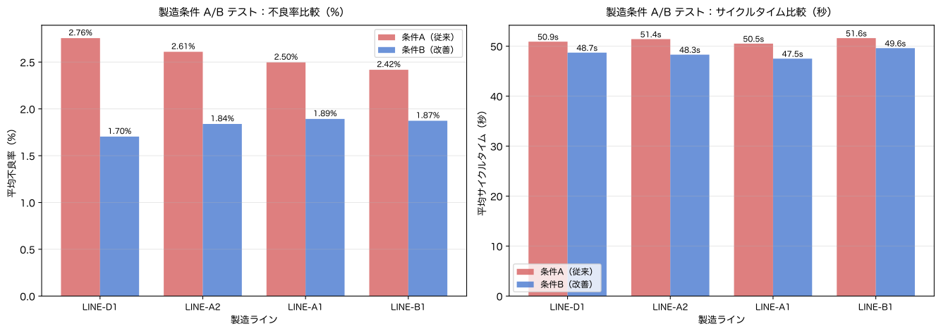

svg

A/Bテスト比較グラフ表示完了（SVG 2/2）

結果の読み取り

不良率: 条件 B（改善：低温・高圧）は条件 A（従来）より平均 0.7pt 程度低い不良率を達成しています。t 統計量が全ラインで 2.0 を超える場合、 5% 水準で統計的に有意な改善と判断できます
サイクルタイム: 条件 B は条件 A より約 3〜4 秒短縮されています。月産 7,800 バッチ × 3.5 秒短縮 = 27,300 秒/月 ≈ 7.6 時間/月の生産効率改善です
グラフ: 全4ラインで条件 B の不良率・サイクルタイムが一貫して低い場合、改善効果の 再現性が高く、量産切り替えの判断材料になります
統計的有意性の確認後、製造コスト・設備投資との費用対効果を評価して量産条件への採用可否を決定します

No.089：機械学習用の特徴量テーブルを作成する

実務での意味

設備異常予知 ML モデルには「過去の状態」を表す時系列特徴量が不可欠です。 SQL のウィンドウ関数を使えば、LAG・移動平均・累積値などの特徴量を Python の前処理なしに DB 上で計算できます。

製造業での活用例：

前バッチのサイクルタイム・アラーム数を特徴量として次バッチの不良率を予測
3バッチ移動平均不良率が閾値を超えたら自動アラートを発行
ML 特徴量テーブルを BI ツールに接続してリアルタイムダッシュボードに活用

分析・モデル化の考え方

時系列特徴量の種類：

特徴量	計算式（SQL）	意味
1 バッチ前の値	`LAG(x, 1) OVER (...)`	直前バッチの状態
3 バッチ移動平均	`AVG(x) OVER (ROWS BETWEEN 2 PRECEDING AND CURRENT ROW)`	短期トレンド
累積不良数	`SUM(defect) OVER (ROWS UNBOUNDED PRECEDING)`	設備劣化の累積

\hat{y}_{t+1} = f\bigl(x_t,\; x_{t-1},\; \bar{x}_{t-2:t},\; \text{cum\_defect}_t\bigr)

これらの特徴量を SQL で計算することで、 Python の pandas 前処理を最小化できます。

Python で確認する

# No.089: ウィンドウ関数で ML 特徴量テーブルを作成

print('=== LINE-A1 × 条件A: ML 特徴量テーブル（LAG + 移動平均 + 累積）===')
q(conn, '''
WITH base AS (
    SELECT batch_id, line_code, experiment_month, group_name,
           condition_temp, condition_pressure,
           input_qty, defect_qty,
           ROUND(defect_qty * 100.0 / input_qty, 3) AS defect_rate,
           cycle_time_sec, alarm_count
    FROM   experiments
)
SELECT batch_id,
       line_code, experiment_month, group_name,
       ROUND(defect_rate, 3)       AS defect_rate,
       cycle_time_sec,
       alarm_count,
       -- LAG 特徴量（1バッチ前）
       LAG(cycle_time_sec, 1) OVER (
           PARTITION BY line_code, group_name
           ORDER BY experiment_month
       )                           AS lag1_cycle_time,
       LAG(alarm_count, 1) OVER (
           PARTITION BY line_code, group_name
           ORDER BY experiment_month
       )                           AS lag1_alarm,
       -- 移動平均特徴量（直近3バッチ）
       ROUND(AVG(cycle_time_sec) OVER (
           PARTITION BY line_code, group_name
           ORDER BY experiment_month
           ROWS BETWEEN 2 PRECEDING AND CURRENT ROW
       ), 2)                       AS ma3_cycle_time,
       ROUND(AVG(alarm_count) OVER (
           PARTITION BY line_code, group_name
           ORDER BY experiment_month
           ROWS BETWEEN 2 PRECEDING AND CURRENT ROW
       ), 2)                       AS ma3_alarm,
       -- 累積不良数
       SUM(defect_qty) OVER (
           PARTITION BY line_code, group_name
           ORDER BY experiment_month
           ROWS UNBOUNDED PRECEDING
       )                           AS cum_defect
FROM   base
WHERE  line_code = 'LINE-A1' AND group_name = 'A'
ORDER  BY experiment_month
''')

=== LINE-A1 × 条件A: ML 特徴量テーブル（LAG + 移動平均 + 累積）===
── SQL ─────────────────────────────────────────
  WITH base AS (
      SELECT batch_id, line_code, experiment_month, group_name,
             condition_temp, condition_pressure,
             input_qty, defect_qty,
             ROUND(defect_qty * 100.0 / input_qty, 3) AS defect_rate,
             cycle_time_sec, alarm_count
      FROM   experiments
  )
  SELECT batch_id,
         line_code, experiment_month, group_name,
         ROUND(defect_rate, 3)       AS defect_rate,
         cycle_time_sec,
         alarm_count,
         -- LAG 特徴量（1バッチ前）
         LAG(cycle_time_sec, 1) OVER (
             PARTITION BY line_code, group_name
             ORDER BY experiment_month
         )                           AS lag1_cycle_time,
         LAG(alarm_count, 1) OVER (
             PARTITION BY line_code, group_name
             ORDER BY experiment_month
         )                           AS lag1_alarm,
         -- 移動平均特徴量（直近3バッチ）
         ROUND(AVG(cycle_time_sec) OVER (
             PARTITION BY line_code, group_name
             ORDER BY experiment_month
             ROWS BETWEEN 2 PRECEDING AND CURRENT ROW
         ), 2)                       AS ma3_cycle_time,
         ROUND(AVG(alarm_count) OVER (
             PARTITION BY line_code, group_name
             ORDER BY experiment_month
             ROWS BETWEEN 2 PRECEDING AND CURRENT ROW
         ), 2)                       AS ma3_alarm,
         -- 累積不良数
         SUM(defect_qty) OVER (
             PARTITION BY line_code, group_name
             ORDER BY experiment_month
             ROWS UNBOUNDED PRECEDING
         )                           AS cum_defect
  FROM   base
  WHERE  line_code = 'LINE-A1' AND group_name = 'A'
  ORDER  BY experiment_month
───────────────────────────────────────────────
shape: (10, 12)
┌──────────┬───────────┬───────────┬───────────┬───┬───────────┬───────────┬───────────┬───────────┐
│ batch_id ┆ line_code ┆ experimen ┆ group_nam ┆ … ┆ lag1_alar ┆ ma3_cycle ┆ ma3_alarm ┆ cum_defec │
│ ---      ┆ ---       ┆ t_month   ┆ e         ┆   ┆ m         ┆ _time     ┆ ---       ┆ t         │
│ str      ┆ str       ┆ ---       ┆ ---       ┆   ┆ ---       ┆ ---       ┆ f64       ┆ ---       │
│          ┆           ┆ str       ┆ str       ┆   ┆ i64       ┆ f64       ┆           ┆ i64       │
╞══════════╪═══════════╪═══════════╪═══════════╪═══╪═══════════╪═══════════╪═══════════╪═══════════╡
│ EXP-001  ┆ LINE-A1   ┆ 2024-01   ┆ A         ┆ … ┆ null      ┆ 53.2      ┆ 1.0       ┆ 13        │
│ EXP-009  ┆ LINE-A1   ┆ 2024-02   ┆ A         ┆ … ┆ 1         ┆ 52.1      ┆ 0.5       ┆ 28        │
│ EXP-017  ┆ LINE-A1   ┆ 2024-03   ┆ A         ┆ … ┆ 0         ┆ 52.13     ┆ 1.0       ┆ 42        │
│ EXP-025  ┆ LINE-A1   ┆ 2024-04   ┆ A         ┆ … ┆ 2         ┆ 50.53     ┆ 1.33      ┆ 57        │
│ EXP-033  ┆ LINE-A1   ┆ 2024-05   ┆ A         ┆ … ┆ 2         ┆ 50.83     ┆ 1.33      ┆ 66        │
│ EXP-041  ┆ LINE-A1   ┆ 2024-06   ┆ A         ┆ … ┆ 0         ┆ 50.5      ┆ 2.0       ┆ 82        │
│ EXP-049  ┆ LINE-A1   ┆ 2024-07   ┆ A         ┆ … ┆ 4         ┆ 50.0      ┆ 2.67      ┆ 98        │
│ EXP-057  ┆ LINE-A1   ┆ 2024-08   ┆ A         ┆ … ┆ 4         ┆ 50.17     ┆ 3.67      ┆ 110       │
│ EXP-065  ┆ LINE-A1   ┆ 2024-09   ┆ A         ┆ … ┆ 3         ┆ 48.8      ┆ 3.33      ┆ 121       │
│ EXP-073  ┆ LINE-A1   ┆ 2024-10   ┆ A         ┆ … ┆ 3         ┆ 50.17     ┆ 2.33      ┆ 131       │
└──────────┴───────────┴───────────┴───────────┴───┴───────────┴───────────┴───────────┴───────────┘
↳ 10 行取得

shape: (10, 12)

batch_id	line_code	experiment_month	group_name	defect_rate	cycle_time_sec	alarm_count	lag1_cycle_time	lag1_alarm	ma3_cycle_time	ma3_alarm	cum_defect
str	str	str	str	f64	f64	i64	f64	i64	f64	f64	i64
”EXP-001"	"LINE-A1"	"2024-01"	"A”	2.529	53.2	1	null	null	53.2	1.0	13
”EXP-009"	"LINE-A1"	"2024-02"	"A”	2.852	51.0	0	53.2	1	52.1	0.5	28
”EXP-017"	"LINE-A1"	"2024-03"	"A”	2.518	52.2	2	51.0	0	52.13	1.0	42
”EXP-025"	"LINE-A1"	"2024-04"	"A”	2.703	48.4	2	52.2	2	50.53	1.33	57
”EXP-033"	"LINE-A1"	"2024-05"	"A”	1.935	51.9	0	48.4	2	50.83	1.33	66
”EXP-041"	"LINE-A1"	"2024-06"	"A”	2.93	51.2	4	51.9	0	50.5	2.0	82
”EXP-049"	"LINE-A1"	"2024-07"	"A”	2.873	46.9	4	51.2	4	50.0	2.67	98
”EXP-057"	"LINE-A1"	"2024-08"	"A”	2.516	52.4	3	46.9	4	50.17	3.67	110
”EXP-065"	"LINE-A1"	"2024-09"	"A”	2.007	47.1	3	52.4	3	48.8	3.33	121
”EXP-073"	"LINE-A1"	"2024-10"	"A”	2.105	51.0	1	47.1	3	50.17	2.33	131

結果の読み取り

lag1_cycle_time と lag1_alarm は 1バッチ前の値です。最初の行（1バッチ目）は前バッチが存在しないため NULL になります
ma3_cycle_time（3バッチ移動平均サイクルタイム）は最初の2行は利用可能なバッチ数が少ないため、実質 1〜2 バッチの平均になります
cum_defect（累積不良数）は設備の消耗・劣化を表す代理変数として使えます。累積が増加するほど次バッチの不良率が上昇する傾向があれば、保全タイミングの判断指標として活用できます
このテーブルをそのまま scikit-learn や LightGBM に渡せます。 NULL を含む最初の 1〜2 行は学習データから除外するのが一般的です

No.090：予測モデル用の学習データを抽出する

実務での意味

機械学習モデルには「特徴量（現在の状態）」と「ラベル（予測したい未来の値）」のペアが必要です。LEAD() を使うことで「現在の状態 → 次バッチの結果」の対応表を SQL のみで作成できます。

製造業での活用例：

現バッチのサイクルタイム・アラーム数を特徴量として次バッチの不良率を予測
label_high_defect = 1（次バッチが高不良率）の判定を二値分類モデルで予測
学習データを SQL で定期自動更新して再学習パイプラインに組み込む

分析・モデル化の考え方

LEAD() でラベルを付与する：

\text{label}_{t} = \begin{cases} 1 & (\text{defect\_rate}_{t+1} > \theta) \\ 0 & (\text{otherwise}) \end{cases}

閾値 $\theta$ はビジネス要件に応じて設定します。例: 不良率 2.5% を超えたバッチを「高不良率」と定義。最後のバッチは $t+1$ が存在しないため、LEAD が NULL となり学習データから除外します。

Python で確認する

# No.090: LEAD を使った予測モデル用ラベル付き学習データの作成

print('=== 特徴量 + ラベル付き学習データ（全ライン × 全グループ）===')
df_ml = q(conn, '''
WITH base AS (
    SELECT batch_id, line_code, experiment_month, group_name,
           condition_temp, condition_pressure,
           ROUND(defect_qty * 100.0 / input_qty, 3) AS defect_rate,
           cycle_time_sec, alarm_count
    FROM   experiments
),
features AS (
    SELECT *,
           LAG(cycle_time_sec, 1) OVER (
               PARTITION BY line_code, group_name
               ORDER BY experiment_month
           )                               AS lag1_cycle_time,
           LAG(alarm_count, 1) OVER (
               PARTITION BY line_code, group_name
               ORDER BY experiment_month
           )                               AS lag1_alarm,
           ROUND(AVG(cycle_time_sec) OVER (
               PARTITION BY line_code, group_name
               ORDER BY experiment_month
               ROWS BETWEEN 2 PRECEDING AND CURRENT ROW
           ), 2)                           AS ma3_cycle_time
    FROM   base
),
labeled AS (
    SELECT *,
           LEAD(defect_rate, 1) OVER (
               PARTITION BY line_code, group_name
               ORDER BY experiment_month
           )                               AS next_defect_rate,
           CASE
               WHEN LEAD(defect_rate, 1) OVER (
                        PARTITION BY line_code, group_name
                        ORDER BY experiment_month
                    ) > 2.5
               THEN 1 ELSE 0
           END                             AS label_high_defect
    FROM   features
)
SELECT batch_id, line_code, group_name, experiment_month,
       ROUND(condition_temp, 1) AS temp,
       ROUND(condition_pressure, 2) AS pressure,
       cycle_time_sec, alarm_count,
       lag1_cycle_time, lag1_alarm, ma3_cycle_time,
       ROUND(next_defect_rate, 3) AS next_dr,
       label_high_defect
FROM   labeled
WHERE  lag1_cycle_time IS NOT NULL
  AND  next_defect_rate IS NOT NULL
ORDER  BY line_code, group_name, experiment_month
LIMIT  20
''')

# ラベル分布の確認
print()
label_counts = df_ml.group_by('label_high_defect').agg(pl.len().alias('count')).sort('label_high_defect')
print('ラベル分布:')
print(label_counts)
print(f'正例率（高不良率）: {df_ml["label_high_defect"].mean() * 100:.1f}%')

=== 特徴量 + ラベル付き学習データ（全ライン × 全グループ）===
── SQL ─────────────────────────────────────────
  WITH base AS (
      SELECT batch_id, line_code, experiment_month, group_name,
             condition_temp, condition_pressure,
             ROUND(defect_qty * 100.0 / input_qty, 3) AS defect_rate,
             cycle_time_sec, alarm_count
      FROM   experiments
  ),
  features AS (
      SELECT *,
             LAG(cycle_time_sec, 1) OVER (
                 PARTITION BY line_code, group_name
                 ORDER BY experiment_month
             )                               AS lag1_cycle_time,
             LAG(alarm_count, 1) OVER (
                 PARTITION BY line_code, group_name
                 ORDER BY experiment_month
             )                               AS lag1_alarm,
             ROUND(AVG(cycle_time_sec) OVER (
                 PARTITION BY line_code, group_name
                 ORDER BY experiment_month
                 ROWS BETWEEN 2 PRECEDING AND CURRENT ROW
             ), 2)                           AS ma3_cycle_time
      FROM   base
  ),
  labeled AS (
      SELECT *,
             LEAD(defect_rate, 1) OVER (
                 PARTITION BY line_code, group_name
                 ORDER BY experiment_month
             )                               AS next_defect_rate,
             CASE
                 WHEN LEAD(defect_rate, 1) OVER (
                          PARTITION BY line_code, group_name
                          ORDER BY experiment_month
                      ) > 2.5
                 THEN 1 ELSE 0
             END                             AS label_high_defect
      FROM   features
  )
  SELECT batch_id, line_code, group_name, experiment_month,
         ROUND(condition_temp, 1) AS temp,
         ROUND(condition_pressure, 2) AS pressure,
         cycle_time_sec, alarm_count,
         lag1_cycle_time, lag1_alarm, ma3_cycle_time,
         ROUND(next_defect_rate, 3) AS next_dr,
         label_high_defect
  FROM   labeled
  WHERE  lag1_cycle_time IS NOT NULL
    AND  next_defect_rate IS NOT NULL
  ORDER  BY line_code, group_name, experiment_month
  LIMIT  20
───────────────────────────────────────────────
shape: (20, 13)
┌──────────┬───────────┬────────────┬────────────┬───┬───────────┬───────────┬─────────┬───────────┐
│ batch_id ┆ line_code ┆ group_name ┆ experiment ┆ … ┆ lag1_alar ┆ ma3_cycle ┆ next_dr ┆ label_hig │
│ ---      ┆ ---       ┆ ---        ┆ _month     ┆   ┆ m         ┆ _time     ┆ ---     ┆ h_defect  │
│ str      ┆ str       ┆ str        ┆ ---        ┆   ┆ ---       ┆ ---       ┆ f64     ┆ ---       │
│          ┆           ┆            ┆ str        ┆   ┆ i64       ┆ f64       ┆         ┆ i64       │
╞══════════╪═══════════╪════════════╪════════════╪═══╪═══════════╪═══════════╪═════════╪═══════════╡
│ EXP-009  ┆ LINE-A1   ┆ A          ┆ 2024-02    ┆ … ┆ 1         ┆ 52.1      ┆ 2.518   ┆ 1         │
│ EXP-017  ┆ LINE-A1   ┆ A          ┆ 2024-03    ┆ … ┆ 0         ┆ 52.13     ┆ 2.703   ┆ 1         │
│ EXP-025  ┆ LINE-A1   ┆ A          ┆ 2024-04    ┆ … ┆ 2         ┆ 50.53     ┆ 1.935   ┆ 0         │
│ EXP-033  ┆ LINE-A1   ┆ A          ┆ 2024-05    ┆ … ┆ 2         ┆ 50.83     ┆ 2.93    ┆ 1         │
│ EXP-041  ┆ LINE-A1   ┆ A          ┆ 2024-06    ┆ … ┆ 0         ┆ 50.5      ┆ 2.873   ┆ 1         │
│ …        ┆ …         ┆ …          ┆ …          ┆ … ┆ …         ┆ …         ┆ …       ┆ …         │
│ EXP-066  ┆ LINE-A1   ┆ B          ┆ 2024-09    ┆ … ┆ 1         ┆ 46.33     ┆ 1.84    ┆ 0         │
│ EXP-011  ┆ LINE-A2   ┆ A          ┆ 2024-02    ┆ … ┆ 1         ┆ 51.2      ┆ 2.282   ┆ 0         │
│ EXP-019  ┆ LINE-A2   ┆ A          ┆ 2024-03    ┆ … ┆ 4         ┆ 51.6      ┆ 2.471   ┆ 0         │
│ EXP-027  ┆ LINE-A2   ┆ A          ┆ 2024-04    ┆ … ┆ 3         ┆ 51.93     ┆ 2.564   ┆ 1         │
│ EXP-035  ┆ LINE-A2   ┆ A          ┆ 2024-05    ┆ … ┆ 3         ┆ 53.3      ┆ 2.5     ┆ 0         │
└──────────┴───────────┴────────────┴────────────┴───┴───────────┴───────────┴─────────┴───────────┘
↳ 20 行取得

ラベル分布:
shape: (2, 2)
┌───────────────────┬───────┐
│ label_high_defect ┆ count │
│ ---               ┆ ---   │
│ i64               ┆ u32   │
╞═══════════════════╪═══════╡
│ 0                 ┆ 14    │
│ 1                 ┆ 6     │
└───────────────────┴───────┘
正例率（高不良率）: 30.0%

結果の読み取り

next_defect_rate が NULL の最後のバッチ（LEAD が参照できない行）と、 lag1_cycle_time が NULL の最初のバッチを除外しているため、利用可能な学習データは各パーティション 8 バッチ分になります
label_high_defect = 1 の割合（正例率）が全体の 30〜50% 程度あればバランスの良い学習データといえます。5% 未満は不均衡データへの対処が必要です
条件 B（改善条件）の正例率は条件 A より低くなります。モデル学習時は group_name を特徴量に含めることで条件の違いを学習できます
このテーブルを定期的に SQL で自動更新し、scikit-learn や LightGBM の model.predict() と組み合わせることでリアルタイム品質予測パイプラインが構築できます

対象ノックを通して見える実務上の示唆

第9章（No.081〜090）の10ノックを通じて、以下の4つの実務示唆が得られます。

示唆1: 顧客分析と製造分析は「同じ SQL 構造」で解ける

コホート分析（MIN(month) + month_offset）やファネル分析（CASE WHEN + SUM）は Web/SaaS 分析で発展した手法ですが、OEM顧客の継続分析 や 製造工程の歩留まり分析 にそのまま適用できます。業種を超えた再利用性が SQL の強みです。

示唆2: A/Bテストは「感覚」から「データ」への転換点

製造条件の改善判断を「現場の感覚」から「t 統計量による有意性検定」に移行することで、経営会議への報告品質が向上し、改善投資の ROI 評価が可能になります。

示唆3: ML 特徴量は SQL で作れる

LAG・移動平均・累積値などの時系列特徴量を SQL で計算することで、 Python の前処理コードが削減され、DB → SQL → モデル の自動化パイプラインが構築できます。

示唆4: 解約・離脱の検出は「LEAD の NULL 判定」が基本

取引停止・設備停止・ライン休止などの「イベントの終わり」を SQL で検出するには LEAD(...) IS NULL AND month < データ末端 のパターンが最も汎用的です。

実務導入する場合に必要なこと

本章の分析を実業務に展開する場合、以下の準備が必要です。

1. データ基盤の整備

必要なデータ	現在の課題	整備のポイント
顧客別月次受注履歴	Excel・販売管理システムに分散	基幹 DB への統合・月次バッチ更新
製造ロット記録	生産管理システムに閉じている	MES との連携・SQL アクセス可能化
設備イベントログ	PLC・センサーログが非構造化	IoT ゲートウェイ経由で DB に蓄積
A/Bテスト記録	実験設計・記録の仕組みがない	実験管理シートの DB 化

2. SQL のバージョン管理と再現性

分析 SQL を Git 管理することで、レビュー・再実行・改訂履歴の追跡が可能になります。本章のパターンをテンプレートとして社内 SQL ライブラリを構築することを推奨します。

3. ML パイプラインへの接続

No.089〜090 で作成した特徴量テーブルを定期実行（例: 毎朝 6:00 のバッチ処理）し、モデルの再学習・推論結果を DB に書き戻すことで、 SQL ベースの品質予測自動化パイプラインが実現します。

まとめ

本章（第9章、No.081〜090）では 応用分析 SQL として以下を実践しました。

カテゴリ	ノック	学んだ SQL パターン
コホート分析	No.081〜083	`WITH + MIN + SUBSTR CAST` で基準月算出、`LEAD IS NULL` で解約判定
ファネル分析	No.084	`CASE WHEN + SUM` で工程ごとの歩留まりを列展開
ログ集計	No.085〜087	`GROUP BY + COUNT/SUM/AVG` で設備ログ・セッション・歩留まりを集計
A/Bテスト	No.088	`GROUP BY group_name` + 分散計算で t 統計量を算出
ML特徴量	No.089〜090	`LAG + AVG/SUM OVER` で時系列特徴量、`LEAD + CASE` でラベル付与

第9章の核心: 応用分析 SQL は「ウィンドウ関数 × CTE × CASE WHEN」の組み合わせで高度な分析パターンを実現します。Web 分析・CRM 分析・製造分析を問わず、同じ SQL 構造が再利用できる点がこれらの手法の強みです。

次章（第10章: No.091〜100）では SQL の可読性向上・性能最適化・設計ベストプラクティスを学びます。

法人向けのご相談

本 notebook で解説した SQL 応用分析（コホート分析・ファネル分析・A/B テスト・ ML 特徴量抽出）を貴社の実データに適用したい場合や、 SQL ベースのデータ分析基盤の構築をご検討の際は、ぜひご相談ください。

📩 お問い合わせ: surikobo.co.jp/contact まずはお気軽にご相談ください。

SQL応用分析テクニックで製造業の意思決定を深掘りする

SQL 応用分析テクニックで製造業の意思決定を深掘りする

SQL 100本ノック 第9章（No.081〜No.090）：応用分析SQL

はじめに：この記事で扱う製造業の実務課題

現場でよくある状況

なぜこの問題は判断が難しいのか

1. コホートの「基準点」の設計

2. ファネルの「縦から横への変換」

3. A/Bテストの「条件別集計」と検定統計量

4. ML特徴量の「ウィンドウ関数による行方向の特徴抽出」

今回扱うノックの全体像

Python 環境の準備

架空データの作成

No.081：コホート分析用のデータを作成する

実務での意味

分析・モデル化の考え方

Python で確認する

結果の読み取り

No.082：月別継続率を計算する

実務での意味

分析・モデル化の考え方

Python で確認する

結果の読み取り

No.083：解約率を計算する

実務での意味

分析・モデル化の考え方

Python で確認する

結果の読み取り

No.084：ファネル分析用のデータを作成する

実務での意味

分析・モデル化の考え方

Python で確認する

結果の読み取り

No.085：ユーザー行動ログを集計する

実務での意味

分析・モデル化の考え方

Python で確認する

結果の読み取り

No.086：セッション数を集計する

実務での意味

分析・モデル化の考え方

Python で確認する

結果の読み取り

No.087：コンバージョン率を計算する

実務での意味

分析・モデル化の考え方

Python で確認する

結果の読み取り

No.088：A/Bテスト結果を集計する

実務での意味

分析・モデル化の考え方

Python で確認する

結果の読み取り

No.089：機械学習用の特徴量テーブルを作成する

実務での意味

分析・モデル化の考え方

Python で確認する

結果の読み取り

No.090：予測モデル用の学習データを抽出する

実務での意味

分析・モデル化の考え方

Python で確認する

結果の読み取り

対象ノックを通して見える実務上の示唆

示唆1: 顧客分析と製造分析は「同じ SQL 構造」で解ける

示唆2: A/Bテストは「感覚」から「データ」への転換点

示唆3: ML 特徴量は SQL で作れる

示唆4: 解約・離脱の検出は「LEAD の NULL 判定」が基本

実務導入する場合に必要なこと

1. データ基盤の整備

2. SQL のバージョン管理と再現性

3. ML パイプラインへの接続

まとめ

法人向けのご相談

Related Posts

製造ラインのデータ品質管理・SQL設計・BI連携を実務に落とし込む

受注KPI・顧客分析・在庫リスク評価をSQLで自動化する

SQLウィンドウ関数で製造ラインの月次トレンドを多角的に分析する

サブクエリ・CTEで製造ラインの異常検知とKPI集計を自動化する

SQLのJOINで工場・部品・検査記録を横断分析する

SQL 100本ノック第9章（No.081〜No.090）：応用分析SQL