
100 Exercises / SQL / 100 Exercise-Ups to SQL for Data Analysis
Deepening manufacturing decision-making with SQL application analysis techniques
Deepening Manufacturing Decision-Making with SQL Applied Analysis Techniques
SQL 100 Exercises Chapter 9 (No.081–No.090): Applied Analysis SQL
This article is No.9chapter in the “100 Exercises for SQL Basics for Data Analysis” series. Chapter 8 (No.071–080) taught the basics of practical data analysis such as SQL for inventory management and RFM analysis. In this chapter, as Applied Analysis SQL, we will cover cohort analysis, funnel analysis, A/B testing, Advanced patterns of data utilization, such as feature extraction for machine learning, are implemented in SQL.
[!NOTE] This material is a notebook previously used by Surikoubo (or personally by the representative, Kazuyama), and has been reconstructed, edited, and published with the company’s permission. All data listed is fictional and has no relation whatsoever to real companies, factories, or figures.
Introduction: Practical Challenges in Manufacturing Covered in This Article
This is a challenge faced by a joint project between the Corporate Planning Department + Production Technology Department of an automotive parts manufacturer.
Analysis of OEM customer order continuity + Manufacturing process optimization + Scientific verification of quality improvement effects
  1. Calculate the recurring order rate by cohort for OEM customers to assess the health of business relationships.
  2. Designing early warning signals for trading suspension risk by identifying the churn month
  3. Funnel analysis of yield at each stage of the manufacturing process (input→ inspection→ shipment)
  4. Quantitatively grasp actual operation status through aggregation of equipment operation logs and production sessions
  5. Statistically aggregate and compare the results of manufacturing condition improvement experiments (A/B tests)
  6. Creating feature tables and training data for equipment anomaly prediction models in SQL
Previously, these analyses were performed individually using Excel or BI tools, Since the data is spread across multiple tables, you can decide which tables to merge and aggregate using which SQL was unclear, and the analysis costs were high.
Applied Analysis Covered in This Chapter: By using SQL patterns, these analyses can be reproduced as SQL It can be standardized and automated.
Common situations on site
| Analysis Theme | Current Challenges | What can be solved with applied SQL |
|---|---|---|
| Cohort Analysis | Manually aggregate customer ledgers and order data by matching them in Excel | Generate cohort base month in WITH + MIN(month) GROUP BY |
| Retention and churn rates | At the end of each month, manually compare the customer list with the previous month via VLOOKUP. | LEAD() Automatically determines cancellation by referring to next month’s order order |
| Funnel Analysis | Copy and paste the values from separate sheets for each process | CASE WHEN + SUM() Yield for each process is arranged in a row. |
| Behavior Log Aggregation | Aggregating from large volumes of logs takes time | GROUP BY + COUNT / SUM Rapid monthly and equipment aggregation |
| A/B Test Aggregation | Manually compare averages and totals by condition for intuitive judgment | GROUP BY group_name automatically calculates conditional statistics |
| ML feature creation | Preprocessing with Python + pandas before adding to the model | Creating time series features in the database using SQL LAG / moving averages |
Applied Analysis SQL enables complex analysis to be completed within a database, You can minimize post-processing in Python and Excel.
Why is this issue so difficult to judge?
Applied Analysis: Let’s organize four points that are common in SQL and tend to stumble.
1. Designing the cohort’s “reference point”
The key to cohort analysis is defining “When to start.”
-- Use each customer's first order month as the baseline (cohort month)
SELECT customer_id, MIN(month) AS cohort_month
FROM orders GROUP BY customer_id
From this cohort_month, calculate “How many months (month_offset)” until now,
Calculate retention rates by cohort.
2. Transformation of the funnel from vertical to horizontal
For funnel analysis, you need to “arrange the number of cases in each process side by side as a column.”
SELECT SUM(input_qty) AS stage0_input,
       SUM(first_pass_qty) AS stage1_first_check,
       SUM(second_pass_qty) AS stage2_second_check
FROM lot_records GROUP BY line_code
3. “Conditional Tabulation” and Test Statistics for A/B Tests
Not only does it provide conditional averages in GROUP BY group_name,
Variance is also necessary for calculating the t test statistic.
Since SQLite does not have a STDEV(), we use .
4. “Extracting Line-Oriented Features Using Window Functions” for ML Features
LAG(alarm_count, 1) the number of alarms from the previous batch,
AVG(cycle_time) OVER (ROWS BETWEEN 2 PRECEDING AND CURRENT ROW)
We calculate the “time series feature” called the 3-batch moving average cycle time in SQL.
Overview of Exercise covered this time
| No. | Titles | Applications in manufacturing |
|---|---|---|
| 081 | Creating data for cohort analysis | Creation of cohort benchmark tables by month for OEM customer transactions |
| 082 | Calculating monthly retention rates | Calculation of Monthly Order Continuity Rates by Cohort |
| 083 | Calculating churn rate | Identifying trading suspension months and calculating monthly churn rates |
| 084 | Create data for funnel analysis | Yield funnel in the manufacturing process (input→ primary inspection→ secondary inspection→ shipment) |
| 085 | Aggregate user behavior logs | Monthly and line-by-line aggregation of equipment event logs (alarms and abnormalities) |
| 086 | Counting session counts | Aggregation of production batch (session) numbers and operating hours |
| 087 | Calculating conversion rates | Calculation of manufacturing yield (good product shipment rate relative to input quantity) |
| 088 | Aggregating A/B Test Results | Verification of the effectiveness of manufacturing condition improvement experiments (new process vs. conventional process) |
| 089 | Creating feature tables for machine learning | Creation of LAG / Moving Average Features for Equipment Anomaly Prediction Models |
| 090 | Extracting training data for predictive models | Extraction of training data (features + labels) from quality prediction models |
Preparing the Python environment
import subprocess, sys
res = subprocess.run(["sw_vers", "-productVersion"], capture_output=True, text=True)
print(f"macOS : {res.stdout.strip()}")
print(f"Python: {sys.version}")
macOS : 26.3
Python: 3.13.1 (main, Dec 3 2024, 17:59:52) [Clang 16.0.0 (clang-1600.0.26.4)]import sqlite3
import numpy as np
import polars as pl
import matplotlib
import matplotlib.pyplot as plt
matplotlib.rcParams['font.family'] = 'Hiragino Maru Gothic Pro'
%config InlineBackend.figure_format = 'svg'
np.random.seed(42)
print(f"sqlite3 : {sqlite3.sqlite_version}")
print(f"polars : {pl.__version__}")
print(f"numpy : {np.__version__}")
print(f"matplotlib: {matplotlib.__version__}")
print()
print("Library loading complete")sqlite3 : 3.47.2
polars : 1.42.1
numpy : 2.5.1
matplotlib: 3.11.0
Library loading completeCreation of Fictional Data
Scenario: Joint analysis project between the Corporate Planning Department + Production Technology Department of an automotive parts manufacturer Analysis Period: January 2023 – December 2024 (24 months) Table Structure: 4 tables
| Table Name | number of cases | Description |
|---|---|---|
customers | 10 items | OEM Customer Master (including cohort and churn months) |
orders | ~170 items | Monthly Order Records (Customer × Months) |
lot_records | 120 items | Manufacturing lot records (process funnels + session information) |
experiments | 80 items | A/B Test Experiment Batch Records |
Design Points:
- Staggered the start months (cohort months) of 10 OEM customers from January 2023 to January 2024.
- Three companies halted transactions midway (used to calculate churn rates by cohort)
- Manufacturing lot records are equipped with process funnels (input→inspection→shipping) for yield analysis.
- A/B testing compares defect rates and cycle times under manufacturing conditions: A (conventional) vs B (improved)
| customer | Trading start month | Contract Cancellation Month | segment |
|---|---|---|---|
| OEM Manufacturers A & B | 2023-01 | None | major hand |
| OEM manufacturer C.D | 2023-03 | None | backbone |
| OEM manufacturer E.F | 2023-06 | None | backbone |
| OEM Manufacturer G | 2023-09 | None | small and medium-sized |
| OEM Manufacturer H | 2023-09 | 2024-06 | Small and medium (contract cancellation) |
| OEM Manufacturer I | 2024-01 | 2024-04 | Small and medium (contract cancellation) |
| OEM Manufacturer J | 2024-01 | 2024-10 | Small and medium (contract cancellation) |
# ─────────────────────────────────────────────────────────────────────────
# SQL Helper Function
# ─────────────────────────────────────────────────────────────────────────
def q(conn, sql):
    '''SQL Run Polars DataFrame Display'''
    print('── SQL ─────────────────────────────────────────')
    for line in sql.strip().split('\n'):
        print(f'  {line}')
    print('───────────────────────────────────────────────')
    cur = conn.execute(sql.strip())
    rows = cur.fetchall()
    cols = [d[0] for d in cur.description]
    data = {col: [row[i] for row in rows] for i, col in enumerate(cols)}
    df = pl.DataFrame(data)
    print(df)
    print(f'↳ {len(rows)} Acquisition of Banking')
    return df

# ─────────────────────────────────────────────────────────────────────────
# Creating in-memory databases (4 tables)
# ─────────────────────────────────────────────────────────────────────────
conn = sqlite3.connect(':memory:')

conn.executescript('''
CREATE TABLE customers (
    customer_id       TEXT PRIMARY KEY,
    customer_name     TEXT NOT NULL,
    first_order_month TEXT NOT NULL,
    cancel_month      TEXT,
    segment           TEXT NOT NULL,
    base_qty          INTEGER NOT NULL,
    unit_price        INTEGER NOT NULL
);
CREATE TABLE orders (
    customer_id  TEXT    NOT NULL,
    month        TEXT    NOT NULL,
    ordered_qty  INTEGER NOT NULL,
    order_amount INTEGER NOT NULL,
    PRIMARY KEY (customer_id, month)
);
CREATE TABLE lot_records (
    lot_id          TEXT    PRIMARY KEY,
    month           TEXT    NOT NULL,
    line_code       TEXT    NOT NULL,
    input_qty       INTEGER NOT NULL,
    first_pass_qty  INTEGER NOT NULL,
    second_pass_qty INTEGER NOT NULL,
    shipped_qty     INTEGER NOT NULL,
    session_minutes INTEGER NOT NULL,
    alarm_count     INTEGER NOT NULL
);
CREATE TABLE experiments (
    batch_id           TEXT  PRIMARY KEY,
    line_code          TEXT  NOT NULL,
    experiment_month   TEXT  NOT NULL,
    group_name         TEXT  NOT NULL,
    condition_temp     REAL  NOT NULL,
    condition_pressure REAL  NOT NULL,
    input_qty          INTEGER NOT NULL,
    defect_qty         INTEGER NOT NULL,
    cycle_time_sec     REAL  NOT NULL,
    alarm_count        INTEGER NOT NULL
);
''')

# ── customers ──────────────────────────────────────────────────────────────
CUSTOMER_CONFIG = [
    # (cid,     cname,           first_m,    cancel_m,   seg,   base_qty, unit_price)
    ('CUS-001', 'OEMManufacturerA', '2023-01', None,      'major hand', 600, 5500),
    ('CUS-002', 'OEMManufacturerB', '2023-01', None,      'major hand', 850, 4800),
    ('CUS-003', 'OEMManufacturerC', '2023-03', None,      'backbone', 380, 3200),
    ('CUS-004', 'OEMManufacturerD', '2023-03', None,      'backbone', 420, 3800),
    ('CUS-005', 'OEMManufacturerE', '2023-06', None,      'backbone', 260, 2900),
    ('CUS-006', 'OEMManufacturerF', '2023-06', None,      'backbone', 340, 3500),
    ('CUS-007', 'OEMManufacturerG', '2023-09', None,      'small and medium-sized', 180, 2200),
    ('CUS-008', 'OEMManufacturerH', '2023-09', '2024-06', 'small and medium-sized', 140, 1800),
    ('CUS-009', 'OEMManufacturerI', '2024-01', '2024-04', 'small and medium-sized', 200, 2100),
    ('CUS-010', 'OEMManufacturerJ', '2024-01', '2024-10', 'small and medium-sized', 170, 1900),
]
conn.executemany('INSERT INTO customers VALUES (?,?,?,?,?,?,?)', CUSTOMER_CONFIG)

# ── orders ─────────────────────────────────────────────────────────────────
np.random.seed(42)
ALL_MONTHS = [f'{y}-{m:02d}' for y in [2023, 2024] for m in range(1, 13)]

order_records = []
for cid, cname, first_m, cancel_m, seg, base_qty, unit_price in CUSTOMER_CONFIG:
    last_m = cancel_m if cancel_m else '2024-12'
    for month in ALL_MONTHS:
        if first_m <= month <= last_m:
            qty = max(50, int(base_qty * (1 + np.random.normal(0, 0.12))))
            amount = qty * unit_price + int(np.random.normal(0, unit_price * 5))
            order_records.append((cid, month, qty, amount))
conn.executemany('INSERT INTO orders VALUES (?,?,?,?)', order_records)

# ── lot_records ────────────────────────────────────────────────────────────
np.random.seed(42)
LINE_CODES_LOT = ['LINE-A1', 'LINE-A2', 'LINE-B1', 'LINE-C1', 'LINE-D1']
MONTHS_2024    = [f'2024-{m:02d}' for m in range(1, 13)]
# (base_input, first_pass_rate, second_pass_rate, ship_rate)
LINE_YIELD = {
    'LINE-A1': (1800, 0.965, 0.982, 0.997),
    'LINE-A2': (1400, 0.958, 0.979, 0.998),
    'LINE-B1': (1700, 0.962, 0.980, 0.997),
    'LINE-C1': (650,  0.943, 0.975, 0.996),  # Nagoya: Low yield
    'LINE-D1': (1500, 0.961, 0.981, 0.998),
}
lot_records_data = []
lot_num = 0
for month in MONTHS_2024:
    for line_code in LINE_CODES_LOT:
        for _ in range(2):  # 2 lots per month
            lot_num += 1
            lot_id = f'LOT-{lot_num:03d}'
            base_input, r1, r2, r3 = LINE_YIELD[line_code]
            input_qty       = max(500, int(base_input * (1 + np.random.normal(0, 0.04))))
            first_pass_qty  = max(400, round(input_qty * r1 * (1 + np.random.normal(0, 0.008))))
            second_pass_qty = max(350, round(first_pass_qty * r2 * (1 + np.random.normal(0, 0.005))))
            shipped_qty     = max(300, round(second_pass_qty * r3))
            session_min     = max(120, int(np.random.normal(280, 35)))
            alarm_cnt       = max(0, int(np.random.poisson(1.2)))
            lot_records_data.append((lot_id, month, line_code,
                                     input_qty, first_pass_qty, second_pass_qty,
                                     shipped_qty, session_min, alarm_cnt))
conn.executemany('INSERT INTO lot_records VALUES (?,?,?,?,?,?,?,?,?)', lot_records_data)

# ── experiments ────────────────────────────────────────────────────────────
np.random.seed(42)
EXP_LINES  = ['LINE-A1', 'LINE-A2', 'LINE-B1', 'LINE-D1']
EXP_MONTHS = [f'2024-{m:02d}' for m in range(1, 11)]  # 2024-01〜10
# (temp, pressure, defect_rate, cycle_time_sec, alarm_lambda)
GROUP_CONFIG = {
    'A': (182.0, 8.4, 0.025, 51.5, 2.1),   # Conventional Conditions
    'B': (176.0, 9.1, 0.018, 48.0, 1.0),   # Conditions for improvement
}
exp_records = []
exp_num = 0
for exp_month in EXP_MONTHS:
    for line_code in EXP_LINES:
        for group_name, (temp, pressure, base_dr, base_ct, alarm_lam) in GROUP_CONFIG.items():
            exp_num += 1
            batch_id   = f'EXP-{exp_num:03d}'
            input_qty  = max(200, int(np.random.normal(500, 30)))
            defect_qty = max(1, round(input_qty * max(0.005, np.random.normal(base_dr, base_dr * 0.15))))
            cycle_time = round(max(30.0, np.random.normal(base_ct, base_ct * 0.05)), 1)
            alarm_cnt  = max(0, int(np.random.poisson(alarm_lam)))
            act_temp   = round(temp + np.random.normal(0, 1.5), 1)
            act_pres   = round(pressure + np.random.normal(0, 0.2), 2)
            exp_records.append((batch_id, line_code, exp_month, group_name,
                                act_temp, act_pres, input_qty, defect_qty, cycle_time, alarm_cnt))
conn.executemany('INSERT INTO experiments VALUES (?,?,?,?,?,?,?,?,?,?)', exp_records)
conn.commit()

# ── Summary ───────────────────────────────────────────────────────────
print('Number of Tables:')
for tbl in ['customers', 'orders', 'lot_records', 'experiments']:
    n = conn.execute(f'SELECT COUNT(*) FROM {tbl}').fetchone()[0]
    print(f'  {tbl:<18}: {n:>4} records')
print()
print('Database creation completed: 4Table')
print()
q(conn, '''
SELECT c.customer_id, c.customer_name, c.first_order_month,
       c.cancel_month, c.segment,
       COUNT(o.month)        AS order_months,
       SUM(o.order_amount)   AS total_amount
FROM   customers c
LEFT JOIN orders o ON c.customer_id = o.customer_id
GROUP  BY c.customer_id
ORDER  BY c.first_order_month, c.customer_id
''')
Number of tables:
Customers: 10 items
Orders: 170 items
lot_records: 120 items
Experiments: 80
Database creation completed: 4 tables
── SQL ─────────────────────────────────────────
SELECT c.customer_id, c.customer_name, c.first_order_month,
c.cancel_month, c.segment,
COUNT(o.month) AS order_months,
SUM(o.order_amount) AS total_amount
FROM customers c
LEFT JOIN orders o ON c.customer_id = o.customer_id
GROUP BY c.customer_id
ORDER BY c.first_order_month, c.customer_id
───────────────────────────────────────────────
shape: (10, 7)
┌─────────────┬──────────────┬──────────────┬──────────────┬─────────┬──────────────┬──────────────┐
│ customer_id ┆ customer_nam ┆ first_order_ ┆ cancel_month ┆ segment ┆ order_months ┆ total_amount │
│ --- ┆ e ┆ month ┆ --- ┆ --- ┆ --- ┆ --- │
│ str ┆ --- ┆ --- ┆ str ┆ str ┆ i64 ┆ i64 │
│ ┆ str ┆ str ┆ ┆ ┆ ┆ │
╞═════════════╪══════════════╪══════════════╪══════════════╪═════════╪══════════════╪══════════════╡
│ CUS-001 ┆ OEMManufacturerA ┆ 2023-01 ┆ null ┆ major hand ┆ 24 ┆ 77082065 │
│ CUS-002 ┆ OEMManufacturerB ┆ 2023-01 ┆ null ┆ major hand ┆ 24 ┆ 96791726 │
│ CUS-003 ┆ OEMManufacturerC ┆ 2023-03 ┆ null ┆ backbone ┆ 22 ┆ 26441246 │
│ CUS-004 ┆ OEMManufacturerD ┆ 2023-03 ┆ null ┆ backbone ┆ 22 ┆ 35034450 │
│ CUS-005 ┆ OEMManufacturerE ┆ 2023-06 ┆ null ┆ backbone ┆ 19 ┆ 14524649 │
│ CUS-006 ┆ OEMManufacturerF ┆ 2023-06 ┆ null ┆ backbone ┆ 19 ┆ 22494795 │
│ CUS-007 ┆ OEMManufacturerG ┆ 2023-09 ┆ null ┆ small and medium-sized ┆ 16 ┆ 6340016 │
│ CUS-008 ┆ OEMManufacturerH ┆ 2023-09 ┆ 2024-06 ┆ small and medium-sized ┆ 10 ┆ 2616893 │
│ CUS-009 ┆ OEMManufacturerI ┆ 2024-01 ┆ 2024-04 ┆ small and medium-sized ┆ 4 ┆ 1837438 │
│ CUS-010 ┆ OEMManufacturerJ ┆ 2024-01 ┆ 2024-10 ┆ small and medium-sized ┆ 10 ┆ 3247924 │
└─────────────┴──────────────┴──────────────┴──────────────┴─────────┴──────────────┴──────────────┘
↳ Obtained in 10 linesshape: (10, 7)
| customer_id | customer_name | first_order_month | cancel_month | segment | order_months | total_amount |
|---|---|---|---|---|---|---|
| str | str | str | str | str | i64 | i64 |
| ”CUS-001" | "OEMManufacturerA" | "2023-01” | null | ”major hand” | 24 | 77082065 |
| ”CUS-002" | "OEMManufacturerB" | "2023-01” | null | ”major hand” | 24 | 96791726 |
| ”CUS-003" | "OEMManufacturerC" | "2023-03” | null | ”backbone” | 22 | 26441246 |
| ”CUS-004" | "OEMManufacturerD" | "2023-03” | null | ”backbone” | 22 | 35034450 |
| ”CUS-005" | "OEMManufacturerE" | "2023-06” | null | ”backbone” | 19 | 14524649 |
| ”CUS-006" | "OEMManufacturerF" | "2023-06” | null | ”backbone” | 19 | 22494795 |
| ”CUS-007" | "OEMManufacturerG" | "2023-09” | null | ”small and medium-sized” | 16 | 6340016 |
| ”CUS-008" | "OEMManufacturerH" | "2023-09" | "2024-06" | "small and medium-sized” | 10 | 2616893 |
| ”CUS-009" | "OEMManufacturerI" | "2024-01" | "2024-04" | "small and medium-sized” | 4 | 1837438 |
| ”CUS-010" | "OEMManufacturerJ" | "2024-01" | "2024-10" | "small and medium-sized” | 10 | 3247924 |
# ── Data overview graph (monthly active customers / order volume trends by cohort)────────────
rows = conn.execute('''
    SELECT o.month,
           c.first_order_month  AS cohort_month,
           COUNT(DISTINCT o.customer_id) AS active_count,
           SUM(o.order_amount)           AS total_amount
    FROM   orders o
    JOIN   customers c ON o.customer_id = c.customer_id
    GROUP  BY o.month, c.first_order_month
    ORDER  BY o.month, c.first_order_month
''').fetchall()

COHORTS       = ['2023-01', '2023-03', '2023-06', '2023-09', '2024-01']
COHORT_LABELS = ['2023-Q1(A・B)', '2023-Q2(C・D)', '2023-H1(E・F)', '2023-H2(G・H)', '2024-Q1(I・J)']
COHORT_COLORS = ['#4878CF', '#6ACC65', '#D65F5F', '#B47CC7', '#C4AD66']
ALL_MONTHS_S  = sorted(set(r[0] for r in rows))
N_M           = len(ALL_MONTHS_S)
MLABELS       = [m[5:] + 'month' for m in ALL_MONTHS_S]

# Monthly active customers (total) and order amounts by cohort
month_active  = {m: 0 for m in ALL_MONTHS_S}
cohort_amount = {c: [0] * N_M for c in COHORTS}
for month, cohort_month, active_count, total_amount in rows:
    month_active[month] += active_count
    if cohort_month in COHORTS:
        mi = ALL_MONTHS_S.index(month)
        cohort_amount[cohort_month][mi] += (total_amount or 0)

fig, axes = plt.subplots(1, 2, figsize=(14, 5))

# Left: Monthly active customers (line line)
ax1 = axes[0]
x   = list(range(N_M))
y   = [month_active[m] for m in ALL_MONTHS_S]
ax1.plot(x, y, marker='o', markersize=4, linewidth=2, color='#4878CF')
for xi, yi in zip(x, y):
    if yi < max(y):
        ax1.annotate(str(yi), (xi, yi), textcoords='offset points', xytext=(0, 6), fontsize=7, ha='center')
ax1.set_title('monthly Trends in the number of active customers (2023〜2024Year)', fontsize=11, pad=10)
ax1.set_xlabel('month', fontsize=10)
ax1.set_ylabel('Number of active customers (companies)', fontsize=10)
ax1.set_xticks(x[::3])
ax1.set_xticklabels([MLABELS[i] for i in range(0, N_M, 3)], fontsize=8)
ax1.set_ylim(0, 13)
ax1.grid(alpha=0.3)

# Right: Monthly Order Value by Cohort (Stacked Bar)
ax2    = axes[1]
bottom = [0.0] * N_M
for cohort, label, color in zip(COHORTS, COHORT_LABELS, COHORT_COLORS):
    vals = [cohort_amount[cohort][i] / 1_000_000 for i in range(N_M)]
    ax2.bar(x, vals, bottom=bottom, color=color, alpha=0.8, label=label, width=0.85)
    bottom = [b + v for b, v in zip(bottom, vals)]
ax2.set_title('By cohort Monthly Order Amount (Stacked Bar)', fontsize=11, pad=10)
ax2.set_xlabel('month', fontsize=10)
ax2.set_ylabel('Order Amount (million yen)', fontsize=10)
ax2.set_xticks(x[::3])
ax2.set_xticklabels([MLABELS[i] for i in range(0, N_M, 3)], fontsize=8)
ax2.legend(fontsize=7, loc='upper left')
ax2.grid(axis='y', alpha=0.3)

plt.tight_layout()
plt.show()
print('Data overview graph display completed (SVG 1/2)')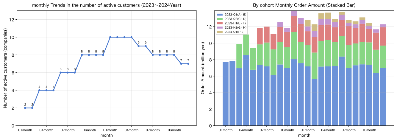
Data overview graph display completed (SVG 1/2)No.081: Creating Data for Cohort Analysis
Meaning in Practice
Cohort Analysis are grouped by common attributes (e.g., transaction start month), This is an analytical method that tracks behavioral changes by group over time.
Examples of use in manufacturing:
- Understanding “Which Months Tend to Concentrate Cancellations” by OEM Customer Transaction Start Month Cohort
- Tracking changes in defect rates at N months after operation in manufacturing equipment introduction cohorts
- Comparing how many months after improvement effects appear by month of start of quality improvement projects
Approach to Analysis and Modeling
The basic structure of cohort analysis is “Who started and when × After the start N ヶCondition of the Moon.”
is the trading start month (cohort month), means the following month, and means N months later.
In SQLite, you extract the year and month from the string using the STRFTIME date calculation
SUBSTR + CAST is more stable.
Check with Python
# No.081: Creation of Cohort Reference Table

print('=== customers Master (with cohort month and cancellation month)===')
q(conn, '''
SELECT customer_id, customer_name, first_order_month,
       cancel_month, segment
FROM   customers
ORDER  BY first_order_month, customer_id
''')

print()
print('=== Cohort Data (customer_id × month × month_offset)===')
q(conn, '''
WITH cohort_base AS (
    SELECT customer_id, first_order_month AS cohort_month
    FROM   customers
),
cohort_data AS (
    SELECT o.customer_id,
           cb.cohort_month,
           o.month,
           (CAST(SUBSTR(o.month, 1, 4) AS INT)
            - CAST(SUBSTR(cb.cohort_month, 1, 4) AS INT)) * 12
           + CAST(SUBSTR(o.month, 6, 2) AS INT)
           - CAST(SUBSTR(cb.cohort_month, 6, 2) AS INT) AS month_offset
    FROM   orders o
    JOIN   cohort_base cb ON o.customer_id = cb.customer_id
)
SELECT cohort_month,
       month_offset,
       COUNT(DISTINCT customer_id) AS active_customers
FROM   cohort_data
GROUP  BY cohort_month, month_offset
ORDER  BY cohort_month, month_offset
LIMIT  20
''')
=== Customers Master (with cohort month and churn month) ===
── SQL ─────────────────────────────────────────
SELECT customer_id, customer_name, first_order_month,
cancel_month, segment
FROM customers
ORDER BY first_order_month, customer_id
───────────────────────────────────────────────
shape: (10, 5)
┌─────────────┬───────────────┬───────────────────┬──────────────┬─────────┐
│ customer_id ┆ customer_name ┆ first_order_month ┆ cancel_month ┆ segment │
│ --- ┆ --- ┆ --- ┆ --- ┆ --- │
│ str ┆ str ┆ str ┆ str ┆ str │
╞═════════════╪═══════════════╪═══════════════════╪══════════════╪═════════╡
│ CUS-001 ┆ OEMManufacturerA ┆ 2023-01 ┆ null ┆ major hand │
│ CUS-002 ┆ OEMManufacturerB ┆ 2023-01 ┆ null ┆ major hand │
│ CUS-003 ┆ OEMManufacturerC ┆ 2023-03 ┆ null ┆ backbone │
│ CUS-004 ┆ OEMManufacturerD ┆ 2023-03 ┆ null ┆ backbone │
│ CUS-005 ┆ OEMManufacturerE ┆ 2023-06 ┆ null ┆ backbone │
│ CUS-006 ┆ OEMManufacturerF ┆ 2023-06 ┆ null ┆ backbone │
│ CUS-007 ┆ OEMManufacturerG ┆ 2023-09 ┆ null ┆ small and medium-sized │
│ CUS-008 ┆ OEMManufacturerH ┆ 2023-09 ┆ 2024-06 ┆ small and medium-sized │
│ CUS-009 ┆ OEMManufacturerI ┆ 2024-01 ┆ 2024-04 ┆ small and medium-sized │
│ CUS-010 ┆ OEMManufacturerJ ┆ 2024-01 ┆ 2024-10 ┆ small and medium-sized │
└─────────────┴───────────────┴───────────────────┴──────────────┴─────────┘
↳ Obtained in 10 lines
=== Cohort Data (customer_id × month × month_offset)===
── SQL ─────────────────────────────────────────
WITH cohort_base AS (
SELECT customer_id, first_order_month AS cohort_month
FROM customers
),
cohort_data AS (
SELECT o.customer_id,
cb.cohort_month,
o.month,
(CAST(SUBSTR(o.month, 1, 4) AS INT)
- CAST(SUBSTR(cb.cohort_month, 1, 4) AS INT)) * 12
+ CAST(SUBSTR(o.month, 6, 2) AS INT)
- CAST(SUBSTR(cb.cohort_month, 6, 2) AS INT) AS month_offset
FROM orders o
JOIN cohort_base cb ON o.customer_id = cb.customer_id
)
SELECT cohort_month,
month_offset,
COUNT(DISTINCT customer_id) AS active_customers
FROM cohort_data
GROUP BY cohort_month, month_offset
ORDER BY cohort_month, month_offset
LIMIT 20
───────────────────────────────────────────────
shape: (20, 3)
┌──────────────┬──────────────┬──────────────────┐
│ cohort_month ┆ month_offset ┆ active_customers │
│ --- ┆ --- ┆ --- │
│ str ┆ i64 ┆ i64 │
╞══════════════╪══════════════╪══════════════════╡
│ 2023-01 ┆ 0 ┆ 2 │
│ 2023-01 ┆ 1 ┆ 2 │
│ 2023-01 ┆ 2 ┆ 2 │
│ 2023-01 ┆ 3 ┆ 2 │
│ 2023-01 ┆ 4 ┆ 2 │
│ … ┆ … ┆ … │
│ 2023-01 ┆ 15 ┆ 2 │
│ 2023-01 ┆ 16 ┆ 2 │
│ 2023-01 ┆ 17 ┆ 2 │
│ 2023-01 ┆ 18 ┆ 2 │
│ 2023-01 ┆ 19 ┆ 2 │
└──────────────┴──────────────┴──────────────────┘
↳ Obtained in 20 linesshape: (20, 3)
| cohort_month | month_offset | active_customers |
|---|---|---|
| str | i64 | i64 |
| ”2023-01” | 0 | 2 |
| ”2023-01” | 1 | 2 |
| ”2023-01” | 2 | 2 |
| ”2023-01” | 3 | 2 |
| ”2023-01” | 4 | 2 |
| … | … | … |
| “2023-01” | 15 | 2 |
| ”2023-01” | 16 | 2 |
| ”2023-01” | 17 | 2 |
| ”2023-01” | 18 | 2 |
| ”2023-01” | 19 | 2 |
Reading the results
customersSetfirst_order_month(cohort month) andcancel_month(churn month) to the master By providing this system, the foundation for cohort analysis is establishedmonth_offsetis calculated using an integer operation of “annual × 12 + monthly difference.”month_offset = 0is the month the trade began, and= 6is six months later- If you aggregate
active_customersby cohort month, You can list how many companies each cohort was active at eachmonth_offsetpoint in time 2023-09The cohort started with two companies (OEM manufacturers G and H), Since H cancels mid-month, the latter half of themonth_offsetwill be limited to one company
No.082: Calculating Monthly Retention Rate
Meaning in Practice
Retention rate (retention rate) refers to “what percentage of customers will still be N months later compared to the start of the cohort?” This KPI indicates whether the transaction is continuing.
Examples of use in manufacturing:
- Identify months when OEM customer retention rates fall below 60% (churn acceleration months) and strengthen sales strategies
- Monitoring the continuity rate of equipment and process improvement programs to measure retention effects
- Using the initial 3–6 month retention rate of new clients as an input variable for contract renewal forecasting
Approach to Analysis and Modeling
Definition of retention rate:
For , retention rate = 100% (everyone is active at the start of the cohort). It decreases over time and plummets in when churn is concentrated.
It is common to create this retention rate table by cohort and visualize it as a Cohort Heatmap.
Check with Python
# No.082: Calculation of Monthly Retention Rate by Cohort

print('=== By cohort Monthly Retention Rate (retention_pct)===')
q(conn, '''
WITH cohort_data AS (
    SELECT o.customer_id,
           c.first_order_month AS cohort_month,
           o.month,
           (CAST(SUBSTR(o.month, 1, 4) AS INT)
            - CAST(SUBSTR(c.first_order_month, 1, 4) AS INT)) * 12
           + CAST(SUBSTR(o.month, 6, 2) AS INT)
           - CAST(SUBSTR(c.first_order_month, 6, 2) AS INT) AS month_offset
    FROM   orders o
    JOIN   customers c ON o.customer_id = c.customer_id
),
cohort_size AS (
    SELECT first_order_month AS cohort_month,
           COUNT(*)          AS cohort_size
    FROM   customers
    GROUP  BY first_order_month
),
active_by_offset AS (
    SELECT cohort_month, month_offset,
           COUNT(DISTINCT customer_id) AS active_count
    FROM   cohort_data
    GROUP  BY cohort_month, month_offset
)
SELECT a.cohort_month,
       a.month_offset,
       a.active_count,
       cs.cohort_size,
       ROUND(a.active_count * 100.0 / cs.cohort_size, 1) AS retention_pct
FROM   active_by_offset a
JOIN   cohort_size cs ON a.cohort_month = cs.cohort_month
ORDER  BY a.cohort_month, a.month_offset
''')
=== Monthly Retention Rate by Cohort (retention_pct) ===
── SQL ─────────────────────────────────────────
WITH cohort_data AS (
SELECT o.customer_id,
c.first_order_month AS cohort_month,
o.month,
(CAST(SUBSTR(o.month, 1, 4) AS INT)
- CAST(SUBSTR(c.first_order_month, 1, 4) AS INT)) * 12
+ CAST(SUBSTR(o.month, 6, 2) AS INT)
- CAST(SUBSTR(c.first_order_month, 6, 2) AS INT) AS month_offset
FROM orders o
JOIN customers c ON o.customer_id = c.customer_id
),
cohort_size AS (
SELECT first_order_month AS cohort_month,
COUNT(*) AS cohort_size
FROM customers
GROUP BY first_order_month
),
active_by_offset AS (
SELECT cohort_month, month_offset,
COUNT(DISTINCT customer_id) AS active_count
FROM cohort_data
GROUP BY cohort_month, month_offset
)
SELECT a.cohort_month,
a.month_offset,
a.active_count,
cs.cohort_size,
ROUND(a.active_count * 100.0 / cs.cohort_size, 1) AS retention_pct
FROM active_by_offset a
JOIN cohort_size cs ON a.cohort_month = cs.cohort_month
ORDER BY a.cohort_month, a.month_offset
───────────────────────────────────────────────
shape: (91, 5)
┌──────────────┬──────────────┬──────────────┬─────────────┬───────────────┐
│ cohort_month ┆ month_offset ┆ active_count ┆ cohort_size ┆ retention_pct │
│ --- ┆ --- ┆ --- ┆ --- ┆ --- │
│ str ┆ i64 ┆ i64 ┆ i64 ┆ f64 │
╞══════════════╪══════════════╪══════════════╪═════════════╪═══════════════╡
│ 2023-01 ┆ 0 ┆ 2 ┆ 2 ┆ 100.0 │
│ 2023-01 ┆ 1 ┆ 2 ┆ 2 ┆ 100.0 │
│ 2023-01 ┆ 2 ┆ 2 ┆ 2 ┆ 100.0 │
│ 2023-01 ┆ 3 ┆ 2 ┆ 2 ┆ 100.0 │
│ 2023-01 ┆ 4 ┆ 2 ┆ 2 ┆ 100.0 │
│ … ┆ … ┆ … ┆ … ┆ … │
│ 2024-01 ┆ 5 ┆ 1 ┆ 2 ┆ 50.0 │
│ 2024-01 ┆ 6 ┆ 1 ┆ 2 ┆ 50.0 │
│ 2024-01 ┆ 7 ┆ 1 ┆ 2 ┆ 50.0 │
│ 2024-01 ┆ 8 ┆ 1 ┆ 2 ┆ 50.0 │
│ 2024-01 ┆ 9 ┆ 1 ┆ 2 ┆ 50.0 │
└──────────────┴──────────────┴──────────────┴─────────────┴───────────────┘
↳ Obtained in 91 rowsshape: (91, 5)
| cohort_month | month_offset | active_count | cohort_size | retention_pct |
|---|---|---|---|---|
| str | i64 | i64 | i64 | f64 |
| ”2023-01” | 0 | 2 | 2 | 100.0 |
| ”2023-01” | 1 | 2 | 2 | 100.0 |
| ”2023-01” | 2 | 2 | 2 | 100.0 |
| ”2023-01” | 3 | 2 | 2 | 100.0 |
| ”2023-01” | 4 | 2 | 2 | 100.0 |
| … | … | … | … | … |
| “2024-01” | 5 | 1 | 2 | 50.0 |
| ”2024-01” | 6 | 1 | 2 | 50.0 |
| ”2024-01” | 7 | 1 | 2 | 50.0 |
| ”2024-01” | 8 | 1 | 2 | 50.0 |
| ”2024-01” | 9 | 1 | 2 | 50.0 |
Reading the results
cohort_sizeis the number of customers in the cohort (the number of customers with the same transaction start month). For example, the2023-09cohort consists of two companies, G and H (cohort_size = 2).- The month of
retention_pct = 100.0(month_offset = 0) is a starting month when everyone is active 2023-09The cohort is around the 9th to 10th month (equivalent to June 2024 when OEM manufacturer H cancels).retention_pctplunges from 100.0% → 50.0%2024-01Cohorts are canceled early by both companies, causing retention rates to drop rapidly. It suggests a review of onboarding strategies for this cohort
No.083: Calculating Churn Rate
Meaning in Practice
Cancellation rate (churn rate) refers to “among active customers, It shows the percentage of customers who stopped trading during that month.
Examples of use in manufacturing:
- Monthly churn rate is monitored as a KPI, and a system has been established for the sales department to respond promptly.
- Identifying leading signals common to cancellation months, such as “sharp decline in order volume” and “rising defect rates”
- Identify the peak seasons for cancellations (fiscal year-end and fiscal year-end) and plan retention measures in advance
Approach to Analysis and Modeling
Definition of churn rate:
Check ‘Do you have orders next month’ in LEAD(month, 1)?
No orders for the next month & not at the data end = the last order month for that cohort = the churn month.
Check with Python
# No.083: Calculating Monthly Churn Rate Using LEAD

print('=== The final order month of the canceled customer (LEAD (Judgment)===')
q(conn, '''
WITH monthly_orders_lead AS (
    SELECT customer_id, month,
           LEAD(month, 1) OVER (
               PARTITION BY customer_id
               ORDER BY month
           ) AS next_month
    FROM   orders
),
churned AS (
    SELECT customer_id,
           month AS churn_month
    FROM   monthly_orders_lead
    WHERE  next_month IS NULL
      AND  month < '2024-12'          -- Data suffix (2024-12) will not be treated as canceled.
)
SELECT ch.customer_id,
       c.customer_name,
       c.first_order_month,
       c.cancel_month AS expected_cancel,
       ch.churn_month AS detected_churn
FROM   churned ch
JOIN   customers c ON ch.customer_id = c.customer_id
ORDER  BY ch.churn_month
''')

print()
print('=== Monthly churn rate (churned / active_at_month × 100)===')
q(conn, '''
WITH monthly_orders_lead AS (
    SELECT customer_id, month,
           LEAD(month, 1) OVER (PARTITION BY customer_id ORDER BY month) AS next_month
    FROM   orders
),
churned AS (
    SELECT month AS churn_month, COUNT(*) AS churned_count
    FROM   monthly_orders_lead
    WHERE  next_month IS NULL AND month < '2024-12'
    GROUP  BY month
),
monthly_active AS (
    SELECT month, COUNT(DISTINCT customer_id) AS active_count
    FROM   orders
    GROUP  BY month
)
SELECT ma.month,
       ma.active_count,
       COALESCE(ch.churned_count, 0) AS churned,
       ROUND(COALESCE(ch.churned_count, 0) * 100.0 / ma.active_count, 1) AS churn_rate_pct
FROM   monthly_active ma
LEFT JOIN churned ch ON ma.month = ch.churn_month
ORDER  BY ma.month
''')
=== Last order month for canceling customers (determined by LEAD) ===
── SQL ─────────────────────────────────────────
WITH monthly_orders_lead AS (
SELECT customer_id, month,
LEAD(month, 1) OVER (
PARTITION BY customer_id
ORDER BY month
) AS next_month
FROM orders
),
churned AS (
SELECT customer_id,
month AS churn_month
FROM monthly_orders_lead
WHERE next_month IS NULL
AND month < '2024-12' -- Data suffix (2024-12) will not be treated as cancellation
)
SELECT ch.customer_id,
c.customer_name,
c.first_order_month,
c.cancel_month AS expected_cancel,
ch.churn_month AS detected_churn
FROM churned ch
JOIN customers c ON ch.customer_id = c.customer_id
ORDER BY ch.churn_month
───────────────────────────────────────────────
shape: (3, 5)
┌─────────────┬───────────────┬───────────────────┬─────────────────┬────────────────┐
│ customer_id ┆ customer_name ┆ first_order_month ┆ expected_cancel ┆ detected_churn │
│ --- ┆ --- ┆ --- ┆ --- ┆ --- │
│ str ┆ str ┆ str ┆ str ┆ str │
╞═════════════╪═══════════════╪═══════════════════╪═════════════════╪════════════════╡
│ CUS-009 ┆ OEMManufacturerI ┆ 2024-01 ┆ 2024-04 ┆ 2024-04 │
│ CUS-008 ┆ OEMManufacturerH ┆ 2023-09 ┆ 2024-06 ┆ 2024-06 │
│ CUS-010 ┆ OEMManufacturerJ ┆ 2024-01 ┆ 2024-10 ┆ 2024-10 │
└─────────────┴───────────────┴───────────────────┴─────────────────┴────────────────┘
↳ Retrieved in 3 lines
=== Monthly churn rate (churned / active_at_month × 100) ===
── SQL ─────────────────────────────────────────
WITH monthly_orders_lead AS (
SELECT customer_id, month,
LEAD(month, 1) OVER (PARTITION BY customer_id ORDER BY month) AS next_month
FROM orders
),
churned AS (
SELECT month AS churn_month, COUNT(*) AS churned_count
FROM monthly_orders_lead
WHERE next_month IS NULL AND month < '2024-12'
GROUP BY month
),
monthly_active AS (
SELECT month, COUNT(DISTINCT customer_id) AS active_count
FROM orders
GROUP BY month
)
SELECT ma.month,
ma.active_count,
COALESCE(ch.churned_count, 0) AS churned,
ROUND(COALESCE(ch.churned_count, 0) * 100.0 / ma.active_count, 1) AS churn_rate_pct
FROM monthly_active ma
LEFT JOIN churned ch ON ma.month = ch.churn_month
ORDER BY ma.month
───────────────────────────────────────────────
shape: (24, 4)
┌─────────┬──────────────┬─────────┬────────────────┐
│ month ┆ active_count ┆ churned ┆ churn_rate_pct │
│ --- ┆ --- ┆ --- ┆ --- │
│ str ┆ i64 ┆ i64 ┆ f64 │
╞═════════╪══════════════╪═════════╪════════════════╡
│ 2023-01 ┆ 2 ┆ 0 ┆ 0.0 │
│ 2023-02 ┆ 2 ┆ 0 ┆ 0.0 │
│ 2023-03 ┆ 4 ┆ 0 ┆ 0.0 │
│ 2023-04 ┆ 4 ┆ 0 ┆ 0.0 │
│ 2023-05 ┆ 4 ┆ 0 ┆ 0.0 │
│ … ┆ … ┆ … ┆ … │
│ 2024-08 ┆ 8 ┆ 0 ┆ 0.0 │
│ 2024-09 ┆ 8 ┆ 0 ┆ 0.0 │
│ 2024-10 ┆ 8 ┆ 1 ┆ 12.5 │
│ 2024-11 ┆ 7 ┆ 0 ┆ 0.0 │
│ 2024-12 ┆ 7 ┆ 0 ┆ 0.0 │
└─────────┴──────────────┴─────────┴────────────────┘
↳ 24 lines obtainedshape: (24, 4)
| month | active_count | churned | churn_rate_pct |
|---|---|---|---|
| str | i64 | i64 | f64 |
| ”2023-01” | 2 | 0 | 0.0 |
| ”2023-02” | 2 | 0 | 0.0 |
| ”2023-03” | 4 | 0 | 0.0 |
| ”2023-04” | 4 | 0 | 0.0 |
| ”2023-05” | 4 | 0 | 0.0 |
| … | … | … | … |
| “2024-08” | 8 | 0 | 0.0 |
| ”2024-09” | 8 | 0 | 0.0 |
| ”2024-10” | 8 | 1 | 12.5 |
| ”2024-11” | 7 | 0 | 0.0 |
| ”2024-12” | 7 | 0 | 0.0 |
Reading the results
- The line where
LEAD(month, 1)isNULLis “the customer’s last order month.”month < '2024-12'By excluding data endpoints in the condition, only true churns can be detected detected_churnandexpected_cancel(cancel_month) coincide, You can check the accuracy of LEAD’s cancellation determination- The monthly churn rate usually ranges from around 0 to 1 per month, Months with concentrated churns (e.g., 2024-04, 2024-06, 2024-10) are visualized
- By examining the “order volume trends of the previous and two months” for the months when churn rates suddenly increased, You can identify early signals of churn.
No.084: Creating Data for Funnel Analysis
Meaning in Practice
Funnel Analysis is about “how much of each stage of the process toward a goal moves to the next stage.” This is an analytical method that visualizes and visualizes these findings.
Examples of use in manufacturing:
- Grasping yield at each stage of the manufacturing funnel (input → primary inspection pass → secondary inspection pass → shipment)
- Quantifying “Which process causes the most quality loss” and setting improvement priorities
- Visualizing differences in process design and equipment capabilities by comparing multiple funnel lines
Approach to Analysis and Modeling
Yield and total yield at each stage of the manufacturing funnel:
Once you know the yield at each stage, you can identify the ‘bottleneck process,’ You can maximize the effectiveness of your improvement investment.
Check with Python
# No.084: Creation of Manufacturing Funnel Data and Calculation of Yield at Each Stage

print('=== By Line Manufacturing Process Funnel (Annual Aggregation)===')
q(conn, '''
SELECT line_code,
       SUM(input_qty)       AS stage0_input,
       SUM(first_pass_qty)  AS stage1_first_check,
       SUM(second_pass_qty) AS stage2_second_check,
       SUM(shipped_qty)     AS stage3_shipped
FROM   lot_records
GROUP  BY line_code
ORDER  BY line_code
''')

print()
print('=== Yield rate for each process (%) and overall yield ===')
q(conn, '''
WITH funnel AS (
    SELECT line_code,
           SUM(input_qty)       AS s0,
           SUM(first_pass_qty)  AS s1,
           SUM(second_pass_qty) AS s2,
           SUM(shipped_qty)     AS s3
    FROM   lot_records
    GROUP  BY line_code
)
SELECT line_code,
       s0 AS input_qty,
       s3 AS shipped_qty,
       ROUND(s1 * 100.0 / s0, 2) AS first_pass_pct,
       ROUND(s2 * 100.0 / s1, 2) AS second_pass_pct,
       ROUND(s3 * 100.0 / s2, 2) AS ship_pct,
       ROUND(s3 * 100.0 / s0, 2) AS overall_yield_pct,
       s0 - s3                   AS total_loss_qty
FROM   funnel
ORDER  BY overall_yield_pct
''')
=== Manufacturing Process Funnel by Line (Annual Summary) ===
── SQL ─────────────────────────────────────────
SELECT line_code,
SUM(input_qty) AS stage0_input,
SUM(first_pass_qty) AS stage1_first_check,
SUM(second_pass_qty) AS stage2_second_check,
SUM(shipped_qty) AS stage3_shipped
FROM lot_records
GROUP BY line_code
ORDER BY line_code
───────────────────────────────────────────────
shape: (5, 5)
┌───────────┬──────────────┬────────────────────┬─────────────────────┬────────────────┐
│ line_code ┆ stage0_input ┆ stage1_first_check ┆ stage2_second_check ┆ stage3_shipped │
│ --- ┆ --- ┆ --- ┆ --- ┆ --- │
│ str ┆ i64 ┆ i64 ┆ i64 ┆ i64 │
╞═══════════╪══════════════╪════════════════════╪═════════════════════╪════════════════╡
│ LINE-A1 ┆ 42905 ┆ 41414 ┆ 40742 ┆ 40622 │
│ LINE-A2 ┆ 33783 ┆ 32370 ┆ 31676 ┆ 31605 │
│ LINE-B1 ┆ 41133 ┆ 39516 ┆ 38753 ┆ 38633 │
│ LINE-C1 ┆ 15530 ┆ 14647 ┆ 14303 ┆ 14252 │
│ LINE-D1 ┆ 35768 ┆ 34382 ┆ 33771 ┆ 33699 │
└───────────┴──────────────┴────────────────────┴─────────────────────┴────────────────┘
↳ Obtained in 5 rows
=== Yield Rate (%) and Overall Yield for Each Process ===
── SQL ─────────────────────────────────────────
WITH funnel AS (
SELECT line_code,
SUM(input_qty) AS s0,
SUM(first_pass_qty) AS s1,
SUM(second_pass_qty) AS s2,
SUM(shipped_qty) AS s3
FROM lot_records
GROUP BY line_code
)
SELECT line_code,
s0 AS input_qty,
s3 AS shipped_qty,
ROUND(s1 * 100.0 / s0, 2) AS first_pass_pct,
ROUND(s2 * 100.0 / s1, 2) AS second_pass_pct,
ROUND(s3 * 100.0 / s2, 2) AS ship_pct,
ROUND(s3 * 100.0 / s0, 2) AS overall_yield_pct,
s0 - s3 AS total_loss_qty
FROM funnel
ORDER BY overall_yield_pct
───────────────────────────────────────────────
shape: (5, 8)
┌───────────┬───────────┬────────────┬────────────┬────────────┬──────────┬────────────┬───────────┐
│ line_code ┆ input_qty ┆ shipped_qt ┆ first_pass ┆ second_pas ┆ ship_pct ┆ overall_yi ┆ total_los │
│ --- ┆ --- ┆ y ┆ _pct ┆ s_pct ┆ --- ┆ eld_pct ┆ s_qty │
│ str ┆ i64 ┆ --- ┆ --- ┆ --- ┆ f64 ┆ --- ┆ --- │
│ ┆ ┆ i64 ┆ f64 ┆ f64 ┆ ┆ f64 ┆ i64 │
╞═══════════╪═══════════╪════════════╪════════════╪════════════╪══════════╪════════════╪═══════════╡
│ LINE-C1 ┆ 15530 ┆ 14252 ┆ 94.31 ┆ 97.65 ┆ 99.64 ┆ 91.77 ┆ 1278 │
│ LINE-A2 ┆ 33783 ┆ 31605 ┆ 95.82 ┆ 97.86 ┆ 99.78 ┆ 93.55 ┆ 2178 │
│ LINE-B1 ┆ 41133 ┆ 38633 ┆ 96.07 ┆ 98.07 ┆ 99.69 ┆ 93.92 ┆ 2500 │
│ LINE-D1 ┆ 35768 ┆ 33699 ┆ 96.13 ┆ 98.22 ┆ 99.79 ┆ 94.22 ┆ 2069 │
│ LINE-A1 ┆ 42905 ┆ 40622 ┆ 96.52 ┆ 98.38 ┆ 99.71 ┆ 94.68 ┆ 2283 │
└───────────┴───────────┴────────────┴────────────┴────────────┴──────────┴────────────┴───────────┘
↳ Obtained in 5 rowsshape: (5, 8)
| line_code | input_qty | shipped_qty | first_pass_pct | second_pass_pct | ship_pct | overall_yield_pct | total_loss_qty |
|---|---|---|---|---|---|---|---|
| str | i64 | i64 | f64 | f64 | f64 | f64 | i64 |
| ”LINE-C1” | 15530 | 14252 | 94.31 | 97.65 | 99.64 | 91.77 | 1278 |
| ”LINE-A2” | 33783 | 31605 | 95.82 | 97.86 | 99.78 | 93.55 | 2178 |
| ”LINE-B1” | 41133 | 38633 | 96.07 | 98.07 | 99.69 | 93.92 | 2500 |
| ”LINE-D1” | 35768 | 33699 | 96.13 | 98.22 | 99.79 | 94.22 | 2069 |
| ”LINE-A1” | 42905 | 40622 | 96.52 | 98.38 | 99.71 | 94.68 | 2283 |
Reading the results
first_pass_pctline with the lowest (first inspection pass rate) (LINE-C1) This is the bottleneck process in the manufacturing funnel. Investing in this directly leads to improved overall yieldoverall_yield_pct(Total Yield) is the product of yields for each process. For example, 96.5% × 98.2% × 99.7% = approximately 94.5%- If you multiply the unit price by the
total_loss_qty(discarded or reworked quantity), the ‘quality loss cost’ It can be calculated. Even with fewer LINE-C1 cases, the loss cost may be relatively high - By aggregating funnel analysis monthly, you can also monitor the “monthly changes in yield”
No.085: Aggregating User Behavior Logs
Meaning in Practice
By aggregating Equipment Event Log (event records such as alarms, warnings, and emergency stops), You can quantitatively grasp the operating status of equipment and trends in abnormalities.
Examples of use in manufacturing:
- Aggregating alarm counts by line and month to prioritize ‘lines with the most alarms’
- Manage alarm density per lot (alarm/lot) as a KPI
- Carefully examining manufacturing records from the month when the number of alarms suddenly increased to identify the cause
Approach to Analysis and Modeling
Definition of alarm density:
The alarm density during normal equipment operation is low (e.g., less than 1 case per lot),
It rises when preventive maintenance timing approaches, equipment deterioration, or process abnormalities.
By tracking alarm_density trends, you can use it as a Preventive maintenance evaluation indicators.
Check with Python
# No.085: Aggregation of Equipment Event Logs (Number of Alarms / Alarm Density)

print('=== By Line Annual Alarm Count and Frequency ===')
q(conn, '''
SELECT line_code,
       COUNT(lot_id)                                       AS lot_count,
       SUM(alarm_count)                                    AS total_alarms,
       ROUND(SUM(alarm_count) * 1.0 / COUNT(lot_id), 2)  AS alarm_density,
       MAX(alarm_count)                                    AS max_alarms_per_lot,
       SUM(CASE WHEN alarm_count = 0 THEN 1 ELSE 0 END)   AS zero_alarm_lots
FROM   lot_records
GROUP  BY line_code
ORDER  BY total_alarms DESC
''')

print()
print('=== monthly Alarm Count Ranking (All Lines, Top Ranking)12Item)===')
q(conn, '''
SELECT month, line_code,
       SUM(alarm_count)  AS monthly_alarms,
       COUNT(lot_id)     AS lots,
       ROUND(SUM(alarm_count) * 1.0 / COUNT(lot_id), 1) AS density
FROM   lot_records
WHERE  alarm_count > 0
GROUP  BY month, line_code
ORDER  BY monthly_alarms DESC
LIMIT  12
''')
=== Annual Number and Frequency of Alarms by Line ===
── SQL ─────────────────────────────────────────
SELECT line_code,
COUNT(lot_id) AS lot_count,
SUM(alarm_count) AS total_alarms,
ROUND(SUM(alarm_count) * 1.0 / COUNT(lot_id), 2) AS alarm_density,
MAX(alarm_count) AS max_alarms_per_lot,
SUM(CASE WHEN alarm_count = 0 THEN 1 ELSE 0 END) AS zero_alarm_lots
FROM lot_records
GROUP BY line_code
ORDER BY total_alarms DESC
───────────────────────────────────────────────
shape: (5, 6)
┌───────────┬───────────┬──────────────┬───────────────┬────────────────────┬─────────────────┐
│ line_code ┆ lot_count ┆ total_alarms ┆ alarm_density ┆ max_alarms_per_lot ┆ zero_alarm_lots │
│ --- ┆ --- ┆ --- ┆ --- ┆ --- ┆ --- │
│ str ┆ i64 ┆ i64 ┆ f64 ┆ i64 ┆ i64 │
╞═══════════╪═══════════╪══════════════╪═══════════════╪════════════════════╪═════════════════╡
│ LINE-B1 ┆ 24 ┆ 34 ┆ 1.42 ┆ 5 ┆ 8 │
│ LINE-D1 ┆ 24 ┆ 26 ┆ 1.08 ┆ 3 ┆ 11 │
│ LINE-A2 ┆ 24 ┆ 26 ┆ 1.08 ┆ 3 ┆ 8 │
│ LINE-C1 ┆ 24 ┆ 25 ┆ 1.04 ┆ 2 ┆ 7 │
│ LINE-A1 ┆ 24 ┆ 23 ┆ 0.96 ┆ 4 ┆ 11 │
└───────────┴───────────┴──────────────┴───────────────┴────────────────────┴─────────────────┘
↳ Obtained in 5 rows
=== Monthly Alarm Count Ranking (Top 12 Across All Lines) ===
── SQL ─────────────────────────────────────────
SELECT month, line_code,
SUM(alarm_count) AS monthly_alarms,
COUNT(lot_id) AS lots,
ROUND(SUM(alarm_count) * 1.0 / COUNT(lot_id), 1) AS density
FROM lot_records
WHERE alarm_count > 0
GROUP BY month, line_code
ORDER BY monthly_alarms DESC
LIMIT 12
───────────────────────────────────────────────
shape: (12, 5)
┌─────────┬───────────┬────────────────┬──────┬─────────┐
│ month ┆ line_code ┆ monthly_alarms ┆ lots ┆ density │
│ --- ┆ --- ┆ --- ┆ --- ┆ --- │
│ str ┆ str ┆ i64 ┆ i64 ┆ f64 │
╞═════════╪═══════════╪════════════════╪══════╪═════════╡
│ 2024-03 ┆ LINE-D1 ┆ 6 ┆ 2 ┆ 3.0 │
│ 2024-06 ┆ LINE-B1 ┆ 6 ┆ 2 ┆ 3.0 │
│ 2024-02 ┆ LINE-B1 ┆ 5 ┆ 1 ┆ 5.0 │
│ 2024-04 ┆ LINE-A2 ┆ 5 ┆ 2 ┆ 2.5 │
│ 2024-04 ┆ LINE-B1 ┆ 5 ┆ 2 ┆ 2.5 │
│ … ┆ … ┆ … ┆ … ┆ … │
│ 2024-06 ┆ LINE-A2 ┆ 4 ┆ 2 ┆ 2.0 │
│ 2024-09 ┆ LINE-B1 ┆ 4 ┆ 2 ┆ 2.0 │
│ 2024-09 ┆ LINE-C1 ┆ 4 ┆ 2 ┆ 2.0 │
│ 2024-11 ┆ LINE-B1 ┆ 4 ┆ 2 ┆ 2.0 │
│ 2024-11 ┆ LINE-C1 ┆ 4 ┆ 2 ┆ 2.0 │
└─────────┴───────────┴────────────────┴──────┴─────────┘
↳ Obtained in 12 linesshape: (12, 5)
| month | line_code | monthly_alarms | lots | density |
|---|---|---|---|---|
| str | str | i64 | i64 | f64 |
| ”2024-03" | "LINE-D1” | 6 | 2 | 3.0 |
| ”2024-06" | "LINE-B1” | 6 | 2 | 3.0 |
| ”2024-02" | "LINE-B1” | 5 | 1 | 5.0 |
| ”2024-04" | "LINE-A2” | 5 | 2 | 2.5 |
| ”2024-04" | "LINE-B1” | 5 | 2 | 2.5 |
| … | … | … | … | … |
| “2024-06" | "LINE-A2” | 4 | 2 | 2.0 |
| ”2024-09" | "LINE-B1” | 4 | 2 | 2.0 |
| ”2024-09" | "LINE-C1” | 4 | 2 | 2.0 |
| ”2024-11" | "LINE-B1” | 4 | 2 | 2.0 |
| ”2024-11" | "LINE-C1” | 4 | 2 | 2.0 |
Reading the results
- The line with the most
total_alarmsis the ‘line with the highest cumulative number of alarms,’ The morelot_countthe lines, the more alarms will naturally occur. It is important to normalize with alarm density (alarm_density) - If there are three or more lots with
max_alarms_per_lot, It is worth thoroughly investigating the condition of the equipment at the time when the lot was carried out - Lines with more
zero_alarm_lots(zero alarm lot size) operate more stably. You can set an improvement activity goal of “zero_alarm_lotsratio of N% or higher” - If the monthly ranking shows that alarms for specific lines are concentrated in a specific month, This serves as a starting point for investigating what happened that month
No.086: Counting the Number of Sessions
Meaning in Practice
Production Session (batch) is a unit of equipment operating to produce one manufacturing lot. By aggregating the number of sessions and operating hours, you can understand the efficiency of equipment utilization.
Examples of use in manufacturing:
- Calculate utilization rates by aggregating monthly session counts and uptime by line
- Monitor changes in average session time (
avg_session_minutes) Detecting Setup Adjustments, Adjustments, and Increased Wait Time - Identify months where actual session times differ from planned uptime
Approach to Analysis and Modeling
Definition of equipment utilization rate (availability):
Assuming a planned monthly operating time of 8 hours/day × 22 days = 10,560 minutes, You can calculate the utilization rate by comparing it to the total monthly session time.
Check with Python
# No.086: Aggregation of Production Sessions and Uptime

PLANNED_MINUTES_MONTH = 8 * 60 * 22  # 8h × 22 days = 10,560 minutes

print('=== By Line Annual Session Summary ===')
q(conn, '''
SELECT line_code,
       COUNT(lot_id)                         AS total_sessions,
       SUM(session_minutes)                  AS total_minutes,
       ROUND(AVG(session_minutes), 1)        AS avg_session_min,
       MIN(session_minutes)                  AS min_session_min,
       MAX(session_minutes)                  AS max_session_min
FROM   lot_records
GROUP  BY line_code
ORDER  BY total_sessions DESC
''')

print()
print('=== monthly Number of sessions × Operating hours (total for all lines)===')
q(conn, '''
SELECT month,
       COUNT(lot_id)              AS monthly_sessions,
       SUM(session_minutes)       AS total_minutes,
       ROUND(AVG(session_minutes), 1) AS avg_minutes
FROM   lot_records
GROUP  BY month
ORDER  BY month
''')

print()
print(f'References: 1Line Planned Operating Hours = {PLANNED_MINUTES_MONTH:,} minutes/Month (8h×22Day)')
=== Annual Session Summary by Line ===
── SQL ─────────────────────────────────────────
SELECT line_code,
COUNT(lot_id) AS total_sessions,
SUM(session_minutes) AS total_minutes,
ROUND(AVG(session_minutes), 1) AS avg_session_min,
MIN(session_minutes) AS min_session_min,
MAX(session_minutes) AS max_session_min
FROM lot_records
GROUP BY line_code
ORDER BY total_sessions DESC
───────────────────────────────────────────────
shape: (5, 6)
┌───────────┬────────────────┬───────────────┬─────────────────┬─────────────────┬─────────────────┐
│ line_code ┆ total_sessions ┆ total_minutes ┆ avg_session_min ┆ min_session_min ┆ max_session_min │
│ --- ┆ --- ┆ --- ┆ --- ┆ --- ┆ --- │
│ str ┆ i64 ┆ i64 ┆ f64 ┆ i64 ┆ i64 │
╞═══════════╪════════════════╪═══════════════╪═════════════════╪═════════════════╪═════════════════╡
│ LINE-D1 ┆ 24 ┆ 6624 ┆ 276.0 ┆ 235 ┆ 324 │
│ LINE-C1 ┆ 24 ┆ 6794 ┆ 283.1 ┆ 186 ┆ 346 │
│ LINE-B1 ┆ 24 ┆ 6499 ┆ 270.8 ┆ 216 ┆ 344 │
│ LINE-A2 ┆ 24 ┆ 6607 ┆ 275.3 ┆ 216 ┆ 316 │
│ LINE-A1 ┆ 24 ┆ 7016 ┆ 292.3 ┆ 198 ┆ 375 │
└───────────┴────────────────┴───────────────┴─────────────────┴─────────────────┴─────────────────┘
↳ Obtained in 5 rows
=== Monthly Number of Sessions × Total Uptime (Total for All Lines) ===
── SQL ─────────────────────────────────────────
SELECT month,
COUNT(lot_id) AS monthly_sessions,
SUM(session_minutes) AS total_minutes,
ROUND(AVG(session_minutes), 1) AS avg_minutes
FROM lot_records
GROUP BY month
ORDER BY month
───────────────────────────────────────────────
shape: (12, 4)
┌─────────┬──────────────────┬───────────────┬─────────────┐
│ month ┆ monthly_sessions ┆ total_minutes ┆ avg_minutes │
│ --- ┆ --- ┆ --- ┆ --- │
│ str ┆ i64 ┆ i64 ┆ f64 │
╞═════════╪══════════════════╪═══════════════╪═════════════╡
│ 2024-01 ┆ 10 ┆ 2906 ┆ 290.6 │
│ 2024-02 ┆ 10 ┆ 2899 ┆ 289.9 │
│ 2024-03 ┆ 10 ┆ 2837 ┆ 283.7 │
│ 2024-04 ┆ 10 ┆ 2896 ┆ 289.6 │
│ 2024-05 ┆ 10 ┆ 2813 ┆ 281.3 │
│ … ┆ … ┆ … ┆ … │
│ 2024-08 ┆ 10 ┆ 2643 ┆ 264.3 │
│ 2024-09 ┆ 10 ┆ 2853 ┆ 285.3 │
│ 2024-10 ┆ 10 ┆ 2641 ┆ 264.1 │
│ 2024-11 ┆ 10 ┆ 2764 ┆ 276.4 │
│ 2024-12 ┆ 10 ┆ 2636 ┆ 263.6 │
└─────────┴──────────────────┴───────────────┴─────────────┘
↳ Obtained in 12 lines
Reference: Planned operating time for one line = 10,560 minutes/month (8h×22 days)Reading the results
total_sessions(Monthly: Total of all lines 24 = 5 lines × 2 batches × 12 months / 12) The schedule is fixed each month (designed in two batches per month). In actual sites, unplanned stops cause fluctuations- Track changes in
avg_session_min(average session time) in trends. The increasing trend is indicated by signals such as “deterioration of setup time” and “speed drop due to equipment deterioration” - By dividing
total_minutesby the planned operating hours (10,560 minutes per line/month), you can calculate the utilization rate. You can report monthly utilization KPIs for each line to management meetings - Months with fewer sessions (such as planned suspensions or consecutive holidays) and months with more sessions (such as overtime and holiday work) Variance analysis helps understand seasonal fluctuations in cost and quality
No.087: Calculating Conversion Rate
Meaning in Practice
Conversion rate in manufacturing is “how many raw materials and work-in-progress are input.” It is a Overall yield rate indicating whether it will be shipped as a good product.
Examples of use in manufacturing:
- Calculate annual and monthly comprehensive yields by line to use as basic data for cost accounting.
- Calculate the ROI of improvement investments by converting the amount of improvement in yield into monetary value
- Quantifying “Which process improvements are most effective” by comparing yields across processes
Approach to Analysis and Modeling
Overall funnel conversion rate (total yield):
Quality costs (disposal and reworking costs) are:
This quality loss cost leads to maximized ROI through improvements invested in the line.
Check with Python
# No.087: Calculation of Manufacturing Yield (Conversion Rate)

print('=== By Line Overall yield rate and breakdowns at each stage ===')
q(conn, '''
WITH funnel AS (
    SELECT lr.line_code,
           SUM(lr.input_qty)         AS s0,
           SUM(lr.first_pass_qty)    AS s1,
           SUM(lr.second_pass_qty)   AS s2,
           SUM(lr.shipped_qty)       AS s3
    FROM   lot_records lr
    GROUP  BY lr.line_code
)
SELECT f.line_code,
       f.s0                             AS input_qty,
       f.s3                             AS shipped_qty,
       f.s0 - f.s3                      AS loss_qty,
       ROUND(f.s1 * 100.0 / f.s0, 2)   AS first_pass_pct,
       ROUND(f.s2 * 100.0 / f.s1, 2)   AS second_pass_pct,
       ROUND(f.s3 * 100.0 / f.s2, 2)   AS ship_pct,
       ROUND(f.s3 * 100.0 / f.s0, 2)   AS overall_yield_pct
FROM   funnel f
ORDER  BY overall_yield_pct
''')

print()
print('=== monthly Overall average yield rate (total for all lines)===')
q(conn, '''
SELECT month,
       SUM(input_qty)  AS monthly_input,
       SUM(shipped_qty) AS monthly_shipped,
       ROUND(SUM(shipped_qty) * 100.0 / SUM(input_qty), 2) AS monthly_yield_pct
FROM   lot_records
GROUP  BY month
ORDER  BY month
''')
=== Overall Yield Rate by Line and Breakdown by Process ===
── SQL ─────────────────────────────────────────
WITH funnel AS (
SELECT lr.line_code,
SUM(lr.input_qty) AS s0,
SUM(lr.first_pass_qty) AS s1,
SUM(lr.second_pass_qty) AS s2,
SUM(lr.shipped_qty) AS s3
FROM lot_records lr
GROUP BY lr.line_code
)
SELECT f.line_code,
f.s0 AS input_qty,
f.s3 AS shipped_qty,
f.s0 - f.s3 AS loss_qty,
ROUND(f.s1 * 100.0 / f.s0, 2) AS first_pass_pct,
ROUND(f.s2 * 100.0 / f.s1, 2) AS second_pass_pct,
ROUND(f.s3 * 100.0 / f.s2, 2) AS ship_pct,
ROUND(f.s3 * 100.0 / f.s0, 2) AS overall_yield_pct
FROM funnel f
ORDER BY overall_yield_pct
───────────────────────────────────────────────
shape: (5, 8)
┌───────────┬───────────┬─────────────┬──────────┬────────────┬────────────┬──────────┬────────────┐
│ line_code ┆ input_qty ┆ shipped_qty ┆ loss_qty ┆ first_pass ┆ second_pas ┆ ship_pct ┆ overall_yi │
│ --- ┆ --- ┆ --- ┆ --- ┆ _pct ┆ s_pct ┆ --- ┆ eld_pct │
│ str ┆ i64 ┆ i64 ┆ i64 ┆ --- ┆ --- ┆ f64 ┆ --- │
│ ┆ ┆ ┆ ┆ f64 ┆ f64 ┆ ┆ f64 │
╞═══════════╪═══════════╪═════════════╪══════════╪════════════╪════════════╪══════════╪════════════╡
│ LINE-C1 ┆ 15530 ┆ 14252 ┆ 1278 ┆ 94.31 ┆ 97.65 ┆ 99.64 ┆ 91.77 │
│ LINE-A2 ┆ 33783 ┆ 31605 ┆ 2178 ┆ 95.82 ┆ 97.86 ┆ 99.78 ┆ 93.55 │
│ LINE-B1 ┆ 41133 ┆ 38633 ┆ 2500 ┆ 96.07 ┆ 98.07 ┆ 99.69 ┆ 93.92 │
│ LINE-D1 ┆ 35768 ┆ 33699 ┆ 2069 ┆ 96.13 ┆ 98.22 ┆ 99.79 ┆ 94.22 │
│ LINE-A1 ┆ 42905 ┆ 40622 ┆ 2283 ┆ 96.52 ┆ 98.38 ┆ 99.71 ┆ 94.68 │
└───────────┴───────────┴─────────────┴──────────┴────────────┴────────────┴──────────┴────────────┘
↳ Obtained in 5 rows
=== Monthly Overall Average Yield Rate (Total for All Lines) ===
── SQL ─────────────────────────────────────────
SELECT month,
SUM(input_qty) AS monthly_input,
SUM(shipped_qty) AS monthly_shipped,
ROUND(SUM(shipped_qty) * 100.0 / SUM(input_qty), 2) AS monthly_yield_pct
FROM lot_records
GROUP BY month
ORDER BY month
───────────────────────────────────────────────
shape: (12, 4)
┌─────────┬───────────────┬─────────────────┬───────────────────┐
│ month ┆ monthly_input ┆ monthly_shipped ┆ monthly_yield_pct │
│ --- ┆ --- ┆ --- ┆ --- │
│ str ┆ i64 ┆ i64 ┆ f64 │
╞═════════╪═══════════════╪═════════════════╪═══════════════════╡
│ 2024-01 ┆ 14179 ┆ 13276 ┆ 93.63 │
│ 2024-02 ┆ 14121 ┆ 13230 ┆ 93.69 │
│ 2024-03 ┆ 13823 ┆ 13020 ┆ 94.19 │
│ 2024-04 ┆ 14278 ┆ 13411 ┆ 93.93 │
│ 2024-05 ┆ 13947 ┆ 13153 ┆ 94.31 │
│ … ┆ … ┆ … ┆ … │
│ 2024-08 ┆ 14049 ┆ 13261 ┆ 94.39 │
│ 2024-09 ┆ 14037 ┆ 13067 ┆ 93.09 │
│ 2024-10 ┆ 14368 ┆ 13452 ┆ 93.62 │
│ 2024-11 ┆ 14347 ┆ 13506 ┆ 94.14 │
│ 2024-12 ┆ 14016 ┆ 13176 ┆ 94.01 │
└─────────┴───────────────┴─────────────────┴───────────────────┘
↳ Obtained in 12 linesshape: (12, 4)
| month | monthly_input | monthly_shipped | monthly_yield_pct |
|---|---|---|---|
| str | i64 | i64 | f64 |
| ”2024-01” | 14179 | 13276 | 93.63 |
| ”2024-02” | 14121 | 13230 | 93.69 |
| ”2024-03” | 13823 | 13020 | 94.19 |
| ”2024-04” | 14278 | 13411 | 93.93 |
| ”2024-05” | 13947 | 13153 | 94.31 |
| … | … | … | … |
| “2024-08” | 14049 | 13261 | 94.39 |
| ”2024-09” | 14037 | 13067 | 93.09 |
| ”2024-10” | 14368 | 13452 | 93.62 |
| ”2024-11” | 14347 | 13506 | 94.14 |
| ”2024-12” | 14016 | 13176 | 94.01 |
Reading the results
- The lowest line of
overall_yield_pct(LINE-C1’s Nagoya factory) This is the top priority for yield improvement. The bottleneck is the low pass rate of the first inspection. - Calculating quality loss costs in
loss_qty × unit pricedirectly affects management decisions. The LINE-D1 (crankshaft, unit price ¥8,500) has a high yield, Since the cost per item is high, it is also necessary to check the priority based on loss amount - Trends in monthly yield rates show that yields decline during summer (July to August), If seasonality can be identified, we can design enhanced measures for that period (enhanced temperature management and quality monitoring)
- By creating a monthly KPI dashboard for conversion rates, The effectiveness of quality improvement activities can be quantitatively monitored.
No.088: Aggregating A/B Test Results
Meaning in Practice
Manufacturing Conditions A/BTest is to compare the “Current Process (A)” and the “Improvement Process (B)” This method uses parallel experiments under the same conditions to statistically evaluate differences in quality indicators and productivity.
Examples of use in manufacturing:
- Quantitative evaluation of the effects of changes in mold temperature and molding pressure on defect rates and cycle times
- Decisions on the Introduction of New Materials and New Processes Based on “Data” Rather Than “Intuition”
- Include the effect size and statistical significance of improvement measures in the management report
Approach to Analysis and Modeling
Statistics for the two-sample t-test (Welch’s t-test without assuming the equation of variance):
Since SQLite does not have a STDEV(), the calculation of variance
is used.
(for degrees of freedom 18–20, the threshold for a 5% significance level is 2.10) This is an estimate of statistical significance.
Check with Python
# No.088: A/B Test Conditional Tabulation and Calculation of t-Statistics

print('=== Manufacturing Conditions A/B Comparison (Defect Rate, Cycle Time, Number of Alarms)===')
df_ab = q(conn, '''
WITH stats AS (
    SELECT line_code,
           group_name,
           COUNT(*)                                              AS n,
           ROUND(AVG(defect_qty * 100.0 / input_qty), 3)        AS mean_dr,
           ROUND(AVG(condition_temp), 1)                        AS mean_temp,
           ROUND(AVG(condition_pressure), 2)                    AS mean_pres,
           ROUND(AVG(cycle_time_sec), 2)                        AS mean_ct,
           SUM(alarm_count)                                      AS total_alarms,
           AVG(defect_qty * 100.0 / input_qty
               * (defect_qty * 100.0 / input_qty))
           - AVG(defect_qty * 100.0 / input_qty)
             * AVG(defect_qty * 100.0 / input_qty)               AS var_dr
    FROM   experiments
    GROUP  BY line_code, group_name
),
ab AS (
    SELECT a.line_code,
           a.mean_dr AS mean_dr_A, a.var_dr AS var_dr_A, a.n AS n_A,
           b.mean_dr AS mean_dr_B, b.var_dr AS var_dr_B, b.n AS n_B,
           a.mean_ct AS mean_ct_A, b.mean_ct AS mean_ct_B,
           a.total_alarms AS alarms_A, b.total_alarms AS alarms_B
    FROM   stats a
    JOIN   stats b ON a.line_code = b.line_code
    WHERE  a.group_name = 'A' AND b.group_name = 'B'
)
SELECT line_code,
       ROUND(mean_dr_A, 3) AS dr_A_pct,
       ROUND(mean_dr_B, 3) AS dr_B_pct,
       ROUND(mean_dr_A - mean_dr_B, 3)      AS dr_diff,
       ROUND((mean_dr_A - mean_dr_B)
             / SQRT(var_dr_A / n_A + var_dr_B / n_B), 2) AS t_stat,
       ROUND(mean_ct_A, 1) AS ct_A_sec,
       ROUND(mean_ct_B, 1) AS ct_B_sec,
       alarms_A, alarms_B
FROM   ab
ORDER  BY t_stat DESC
''')
=== Manufacturing Condition A/B Comparison (Defect Rate, Cycle Time, Number of Alarms) ===
── SQL ─────────────────────────────────────────
WITH stats AS (
SELECT line_code,
group_name,
COUNT(*) AS n,
ROUND(AVG(defect_qty * 100.0 / input_qty), 3) AS mean_dr,
ROUND(AVG(condition_temp), 1) AS mean_temp,
ROUND(AVG(condition_pressure), 2) AS mean_pres,
ROUND(AVG(cycle_time_sec), 2) AS mean_ct,
SUM(alarm_count) AS total_alarms,
AVG(defect_qty * 100.0 / input_qty
* (defect_qty * 100.0 / input_qty))
- AVG(defect_qty * 100.0 / input_qty)
* AVG(defect_qty * 100.0 / input_qty) AS var_dr
FROM experiments
GROUP BY line_code, group_name
),
ab AS (
SELECT a.line_code,
a.mean_dr AS mean_dr_A, a.var_dr AS var_dr_A, a.n AS n_A,
b.mean_dr AS mean_dr_B, b.var_dr AS var_dr_B, b.n AS n_B,
a.mean_ct AS mean_ct_A, b.mean_ct AS mean_ct_B,
a.total_alarms AS alarms_A, b.total_alarms AS alarms_B
FROM stats a
JOIN stats b ON a.line_code = b.line_code
WHERE a.group_name = 'A' AND b.group_name = 'B'
)
SELECT line_code,
ROUND(mean_dr_A, 3) AS dr_A_pct,
ROUND(mean_dr_B, 3) AS dr_B_pct,
ROUND(mean_dr_A - mean_dr_B, 3) AS dr_diff,
ROUND((mean_dr_A - mean_dr_B)
/ SQRT(var_dr_A / n_A + var_dr_B / n_B), 2) AS t_stat,
ROUND(mean_ct_A, 1) AS ct_A_sec,
ROUND(mean_ct_B, 1) AS ct_B_sec,
alarms_A, alarms_B
FROM ab
ORDER BY t_stat DESC
───────────────────────────────────────────────
shape: (4, 9)
┌───────────┬──────────┬──────────┬─────────┬───┬──────────┬──────────┬──────────┬──────────┐
│ line_code ┆ dr_A_pct ┆ dr_B_pct ┆ dr_diff ┆ … ┆ ct_A_sec ┆ ct_B_sec ┆ alarms_A ┆ alarms_B │
│ --- ┆ --- ┆ --- ┆ --- ┆ ┆ --- ┆ --- ┆ --- ┆ --- │
│ str ┆ f64 ┆ f64 ┆ f64 ┆ ┆ f64 ┆ f64 ┆ i64 ┆ i64 │
╞═══════════╪══════════╪══════════╪═════════╪═══╪══════════╪══════════╪══════════╪══════════╡
│ LINE-D1 ┆ 2.756 ┆ 1.704 ┆ 1.052 ┆ … ┆ 50.9 ┆ 48.7 ┆ 16 ┆ 8 │
│ LINE-A2 ┆ 2.61 ┆ 1.839 ┆ 0.771 ┆ … ┆ 51.4 ┆ 48.3 ┆ 14 ┆ 9 │
│ LINE-A1 ┆ 2.497 ┆ 1.893 ┆ 0.604 ┆ … ┆ 50.5 ┆ 47.5 ┆ 20 ┆ 9 │
│ LINE-B1 ┆ 2.418 ┆ 1.873 ┆ 0.545 ┆ … ┆ 51.6 ┆ 49.6 ┆ 15 ┆ 10 │
└───────────┴──────────┴──────────┴─────────┴───┴──────────┴──────────┴──────────┴──────────┘
↳ Obtained in 4 lines# No.088 Visualization: Comparison of Defect Rates and Cycle Times under Conditions A vs B (4 Lines)
ab_rows = df_ab.to_dicts()
LINES_4 = [r['line_code'] for r in ab_rows]
dr_A = [r['dr_A_pct'] for r in ab_rows]
dr_B = [r['dr_B_pct'] for r in ab_rows]
ct_A = [r['ct_A_sec'] for r in ab_rows]
ct_B = [r['ct_B_sec'] for r in ab_rows]
x = range(len(LINES_4))
w = 0.38
col_A = '#D65F5F'
col_B = '#4878CF'
fig, axes = plt.subplots(1, 2, figsize=(14, 5))
# Left: Defect rate comparison
ax1 = axes[0]
b1 = ax1.bar([xi - w/2 for xi in x], dr_A, w, color=col_A, alpha=0.8, label='conditionA(Conventional)')
b2 = ax1.bar([xi + w/2 for xi in x], dr_B, w, color=col_B, alpha=0.8, label='conditionB(Improvement)')
for bar, val in zip(list(b1) + list(b2), dr_A + dr_B):
ax1.text(bar.get_x() + bar.get_width()/2, bar.get_height() + 0.02,
f'{val:.2f}%', ha='center', va='bottom', fontsize=8)
ax1.set_title('Manufacturing Conditions A/B Test: Defect rate comparison (%)', fontsize=11, pad=10)
ax1.set_xlabel('Production Line', fontsize=10)
ax1.set_ylabel('Average defect rate (%)', fontsize=10)
ax1.set_xticks(list(x))
ax1.set_xticklabels(LINES_4, fontsize=9)
ax1.legend(fontsize=9)
ax1.grid(axis='y', alpha=0.3)
# Right: Cycle time comparison
ax2 = axes[1]
b3 = ax2.bar([xi - w/2 for xi in x], ct_A, w, color=col_A, alpha=0.8, label='conditionA(Conventional)')
b4 = ax2.bar([xi + w/2 for xi in x], ct_B, w, color=col_B, alpha=0.8, label='conditionB(Improvement)')
for bar, val in zip(list(b3) + list(b4), ct_A + ct_B):
ax2.text(bar.get_x() + bar.get_width()/2, bar.get_height() + 0.2,
f'{val:.1f}s', ha='center', va='bottom', fontsize=8)
ax2.set_title('Manufacturing Conditions A/B Test: Cycle time comparison (seconds)', fontsize=11, pad=10)
ax2.set_xlabel('Production Line', fontsize=10)
ax2.set_ylabel('Average cycle time (seconds)', fontsize=10)
ax2.set_xticks(list(x))
ax2.set_xticklabels(LINES_4, fontsize=9)
ax2.legend(fontsize=9)
ax2.grid(axis='y', alpha=0.3)
plt.tight_layout()
plt.show()
print('A/BTest comparison graph display completed (SVG 2/2)')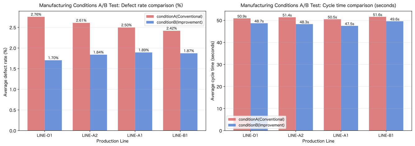
A/B Test Comparison Graph Display Complete (SVG 2/2)Reading the results
- defect rate: Condition B (Improved: Low Temperature and High Pressure) is on average about 0.7 pt lower than Condition A (Conventional) We have achieved a defect rate. If the t statistic exceeds 2.0 across all lines, At the 5% level, it can be considered a statistically significant improvement.
- cycle time: Condition B is about 3–4 seconds shorter than Condition A. Monthly production of 7,800 batches × 3.5 seconds reduction = 27,300 seconds/month ≈ 7.6 hours/month of production efficiency improvement
- graph: If the defect rate and cycle time for condition B are consistently low across all four lines, The reproducibility of improvement effects is high, making it a key factor in deciding when switching to mass production.
- After confirming statistical significance, we evaluated the cost-effectiveness against manufacturing costs and capital investment. We will decide whether to accept the mass production conditions
No.089: Creating a Feature Table for Machine Learning
Meaning in Practice
Equipment Anomaly Prediction ML Model is essential for time series features that represent the “past state.” By using SQL window functions, you can You can compute on the database without Python preprocessing.
Examples of use in manufacturing:
- Using the cycle time alarm count of the previous batch as a feature to predict the defect rate of the next batch
- Automatic alerts are issued when the three-batch moving average defect rate exceeds the threshold
- Connect ML feature tables to BI tools and utilize them for real-time dashboards
Approach to Analysis and Modeling
Types of Time Series Features:
| Feature | Formula (SQL) | Meaning |
|---|---|---|
| 1 Value before batch | LAG(x, 1) OVER (...) | Status of the last-minute batch |
| 3 Batch Moving Average | AVG(x) OVER (ROWS BETWEEN 2 PRECEDING AND CURRENT ROW) | Short-term trends |
| Cumulative number of defects | SUM(defect) OVER (ROWS UNBOUNDED PRECEDING) | Accumulation of equipment deterioration |
By calculating these features in SQL, You can minimize the preprocessing of pandas in Python.
Check with Python
# No.089: Creating an ML Feature Table with Window Functions

print('=== LINE-A1 × conditionA: ML Feature Table (LAG + moving average + Accumulated)===')
q(conn, '''
WITH base AS (
    SELECT batch_id, line_code, experiment_month, group_name,
           condition_temp, condition_pressure,
           input_qty, defect_qty,
           ROUND(defect_qty * 100.0 / input_qty, 3) AS defect_rate,
           cycle_time_sec, alarm_count
    FROM   experiments
)
SELECT batch_id,
       line_code, experiment_month, group_name,
       ROUND(defect_rate, 3)       AS defect_rate,
       cycle_time_sec,
       alarm_count,
       -- LAG Feature (1Before the badge)
       LAG(cycle_time_sec, 1) OVER (
           PARTITION BY line_code, group_name
           ORDER BY experiment_month
       )                           AS lag1_cycle_time,
       LAG(alarm_count, 1) OVER (
           PARTITION BY line_code, group_name
           ORDER BY experiment_month
       )                           AS lag1_alarm,
       -- Moving Average Feature (Most Recent3Badge)
       ROUND(AVG(cycle_time_sec) OVER (
           PARTITION BY line_code, group_name
           ORDER BY experiment_month
           ROWS BETWEEN 2 PRECEDING AND CURRENT ROW
       ), 2)                       AS ma3_cycle_time,
       ROUND(AVG(alarm_count) OVER (
           PARTITION BY line_code, group_name
           ORDER BY experiment_month
           ROWS BETWEEN 2 PRECEDING AND CURRENT ROW
       ), 2)                       AS ma3_alarm,
       -- Cumulative number of defects
       SUM(defect_qty) OVER (
           PARTITION BY line_code, group_name
           ORDER BY experiment_month
           ROWS UNBOUNDED PRECEDING
       )                           AS cum_defect
FROM   base
WHERE  line_code = 'LINE-A1' AND group_name = 'A'
ORDER  BY experiment_month
''')
=== LINE-A1 × Condition A: ML feature table (LAG + moving average + cumulative) ===
── SQL ─────────────────────────────────────────
WITH base AS (
SELECT batch_id, line_code, experiment_month, group_name,
condition_temp, condition_pressure,
input_qty, defect_qty,
ROUND(defect_qty * 100.0 / input_qty, 3) AS defect_rate,
cycle_time_sec, alarm_count
FROM experiments
)
SELECT batch_id,
line_code, experiment_month, group_name,
ROUND(defect_rate, 3) AS defect_rate,
cycle_time_sec,
alarm_count,
-- LAG feature (1 batch ago)
LAG(cycle_time_sec, 1) OVER (
PARTITION BY line_code, group_name
ORDER BY experiment_month
) AS lag1_cycle_time,
LAG(alarm_count, 1) OVER (
PARTITION BY line_code, group_name
ORDER BY experiment_month
) AS lag1_alarm,
-- Moving Average Feature (Last 3 Batches)
ROUND(AVG(cycle_time_sec) OVER (
PARTITION BY line_code, group_name
ORDER BY experiment_month
ROWS BETWEEN 2 PRECEDING AND CURRENT ROW
), 2) AS ma3_cycle_time,
ROUND(AVG(alarm_count) OVER (
PARTITION BY line_code, group_name
ORDER BY experiment_month
ROWS BETWEEN 2 PRECEDING AND CURRENT ROW
), 2) AS ma3_alarm,
-- Cumulative Defects
SUM(defect_qty) OVER (
PARTITION BY line_code, group_name
ORDER BY experiment_month
ROWS UNBOUNDED PRECEDING
) AS cum_defect
FROM base
WHERE line_code = 'LINE-A1' AND group_name = 'A'
ORDER BY experiment_month
───────────────────────────────────────────────
shape: (10, 12)
┌──────────┬───────────┬───────────┬───────────┬───┬───────────┬───────────┬───────────┬───────────┐
│ batch_id ┆ line_code ┆ experimen ┆ group_nam ┆ … ┆ lag1_alar ┆ ma3_cycle ┆ ma3_alarm ┆ cum_defec │
│ --- ┆ --- ┆ t_month ┆ e ┆ ┆ m ┆ _time ┆ --- ┆ t │
│ str ┆ str ┆ --- ┆ --- ┆ ┆ --- ┆ --- ┆ f64 ┆ --- │
│ ┆ ┆ str ┆ str ┆ ┆ i64 ┆ f64 ┆ ┆ i64 │
╞══════════╪═══════════╪═══════════╪═══════════╪═══╪═══════════╪═══════════╪═══════════╪═══════════╡
│ EXP-001 ┆ LINE-A1 ┆ 2024-01 ┆ A ┆ … ┆ null ┆ 53.2 ┆ 1.0 ┆ 13 │
│ EXP-009 ┆ LINE-A1 ┆ 2024-02 ┆ A ┆ … ┆ 1 ┆ 52.1 ┆ 0.5 ┆ 28 │
│ EXP-017 ┆ LINE-A1 ┆ 2024-03 ┆ A ┆ … ┆ 0 ┆ 52.13 ┆ 1.0 ┆ 42 │
│ EXP-025 ┆ LINE-A1 ┆ 2024-04 ┆ A ┆ … ┆ 2 ┆ 50.53 ┆ 1.33 ┆ 57 │
│ EXP-033 ┆ LINE-A1 ┆ 2024-05 ┆ A ┆ … ┆ 2 ┆ 50.83 ┆ 1.33 ┆ 66 │
│ EXP-041 ┆ LINE-A1 ┆ 2024-06 ┆ A ┆ … ┆ 0 ┆ 50.5 ┆ 2.0 ┆ 82 │
│ EXP-049 ┆ LINE-A1 ┆ 2024-07 ┆ A ┆ … ┆ 4 ┆ 50.0 ┆ 2.67 ┆ 98 │
│ EXP-057 ┆ LINE-A1 ┆ 2024-08 ┆ A ┆ … ┆ 4 ┆ 50.17 ┆ 3.67 ┆ 110 │
│ EXP-065 ┆ LINE-A1 ┆ 2024-09 ┆ A ┆ … ┆ 3 ┆ 48.8 ┆ 3.33 ┆ 121 │
│ EXP-073 ┆ LINE-A1 ┆ 2024-10 ┆ A ┆ … ┆ 3 ┆ 50.17 ┆ 2.33 ┆ 131 │
└──────────┴───────────┴───────────┴───────────┴───┴───────────┴───────────┴───────────┴───────────┘
↳ Obtained in 10 linesshape: (10, 12)
| batch_id | line_code | experiment_month | group_name | defect_rate | cycle_time_sec | alarm_count | lag1_cycle_time | lag1_alarm | ma3_cycle_time | ma3_alarm | cum_defect |
|---|---|---|---|---|---|---|---|---|---|---|---|
| str | str | str | str | f64 | f64 | i64 | f64 | i64 | f64 | f64 | i64 |
| ”EXP-001" | "LINE-A1" | "2024-01" | "A” | 2.529 | 53.2 | 1 | null | null | 53.2 | 1.0 | 13 |
| ”EXP-009" | "LINE-A1" | "2024-02" | "A” | 2.852 | 51.0 | 0 | 53.2 | 1 | 52.1 | 0.5 | 28 |
| ”EXP-017" | "LINE-A1" | "2024-03" | "A” | 2.518 | 52.2 | 2 | 51.0 | 0 | 52.13 | 1.0 | 42 |
| ”EXP-025" | "LINE-A1" | "2024-04" | "A” | 2.703 | 48.4 | 2 | 52.2 | 2 | 50.53 | 1.33 | 57 |
| ”EXP-033" | "LINE-A1" | "2024-05" | "A” | 1.935 | 51.9 | 0 | 48.4 | 2 | 50.83 | 1.33 | 66 |
| ”EXP-041" | "LINE-A1" | "2024-06" | "A” | 2.93 | 51.2 | 4 | 51.9 | 0 | 50.5 | 2.0 | 82 |
| ”EXP-049" | "LINE-A1" | "2024-07" | "A” | 2.873 | 46.9 | 4 | 51.2 | 4 | 50.0 | 2.67 | 98 |
| ”EXP-057" | "LINE-A1" | "2024-08" | "A” | 2.516 | 52.4 | 3 | 46.9 | 4 | 50.17 | 3.67 | 110 |
| ”EXP-065" | "LINE-A1" | "2024-09" | "A” | 2.007 | 47.1 | 3 | 52.4 | 3 | 48.8 | 3.33 | 121 |
| ”EXP-073" | "LINE-A1" | "2024-10" | "A” | 2.105 | 51.0 | 1 | 47.1 | 3 | 50.17 | 2.33 | 131 |
Reading the results
lag1_cycle_timeandlag1_alarmare values from one batch earlier. The first row (first batch) isNULLbecause there is no previous batchma3_cycle_time(3-batch moving average cycle time) has the first two lines Because the number of available batches is small, the average is essentially 1 to 2 batchescum_defect(cumulative defects) can be used as a proxy variable to represent equipment wear and deterioration. If the defect rate for the next batch tends to rise as the cumulative amount increases, It can be used as an indicator for determining the timing of conservation.- You can pass this table directly to scikit-learn or LightGBM.
It is common to exclude the first 1 to 2 lines containing
NULLfrom the training data
No.090: Extracting Training Data for Predictive Models
Meaning in Practice
Machine learning models have “Feature (current state)” and “Label (the value of the future you want to predict).”
A pair is required. By using LEAD(), →you can
You can create compatibility tables using only SQL.
Examples of use in manufacturing:
- Using the cycle time alarm count of the current batch as a feature, the defect rate for the next batch is predicted.
- Predicting
label_high_defect = 1(the next batch with high defect rate) using a binary classification model - Regularly and automatically update training data in SQL and incorporate it into the retraining pipeline
Approach to Analysis and Modeling
Label with LEAD():
Threshold is set according to business requirements.
Example: Batches with a defect rate exceeding 2.5% are defined as “high defect rate.”
The last batch has no , so LEAD becomes NULL and is excluded from the training data.
Check with Python
# No.090: Creation of Labeled Training Data for Predictive Models Using LEAD

print('=== Feature + Labeled training data (all lines) × All groups)===')
df_ml = q(conn, '''
WITH base AS (
    SELECT batch_id, line_code, experiment_month, group_name,
           condition_temp, condition_pressure,
           ROUND(defect_qty * 100.0 / input_qty, 3) AS defect_rate,
           cycle_time_sec, alarm_count
    FROM   experiments
),
features AS (
    SELECT *,
           LAG(cycle_time_sec, 1) OVER (
               PARTITION BY line_code, group_name
               ORDER BY experiment_month
           )                               AS lag1_cycle_time,
           LAG(alarm_count, 1) OVER (
               PARTITION BY line_code, group_name
               ORDER BY experiment_month
           )                               AS lag1_alarm,
           ROUND(AVG(cycle_time_sec) OVER (
               PARTITION BY line_code, group_name
               ORDER BY experiment_month
               ROWS BETWEEN 2 PRECEDING AND CURRENT ROW
           ), 2)                           AS ma3_cycle_time
    FROM   base
),
labeled AS (
    SELECT *,
           LEAD(defect_rate, 1) OVER (
               PARTITION BY line_code, group_name
               ORDER BY experiment_month
           )                               AS next_defect_rate,
           CASE
               WHEN LEAD(defect_rate, 1) OVER (
                        PARTITION BY line_code, group_name
                        ORDER BY experiment_month
                    ) > 2.5
               THEN 1 ELSE 0
           END                             AS label_high_defect
    FROM   features
)
SELECT batch_id, line_code, group_name, experiment_month,
       ROUND(condition_temp, 1) AS temp,
       ROUND(condition_pressure, 2) AS pressure,
       cycle_time_sec, alarm_count,
       lag1_cycle_time, lag1_alarm, ma3_cycle_time,
       ROUND(next_defect_rate, 3) AS next_dr,
       label_high_defect
FROM   labeled
WHERE  lag1_cycle_time IS NOT NULL
  AND  next_defect_rate IS NOT NULL
ORDER  BY line_code, group_name, experiment_month
LIMIT  20
''')

# Checking label distribution
print()
label_counts = df_ml.group_by('label_high_defect').agg(pl.len().alias('count')).sort('label_high_defect')
print('Label distribution:')
print(label_counts)
print(f'Positive Rate (High Defect Rate): {df_ml["label_high_defect"].mean() * 100:.1f}%')
=== Features + Labeled Training Data (All Lines × All Groups) ===
── SQL ─────────────────────────────────────────
WITH base AS (
SELECT batch_id, line_code, experiment_month, group_name,
condition_temp, condition_pressure,
ROUND(defect_qty * 100.0 / input_qty, 3) AS defect_rate,
cycle_time_sec, alarm_count
FROM experiments
),
features AS (
SELECT *,
LAG(cycle_time_sec, 1) OVER (
PARTITION BY line_code, group_name
ORDER BY experiment_month
) AS lag1_cycle_time,
LAG(alarm_count, 1) OVER (
PARTITION BY line_code, group_name
ORDER BY experiment_month
) AS lag1_alarm,
ROUND(AVG(cycle_time_sec) OVER (
PARTITION BY line_code, group_name
ORDER BY experiment_month
ROWS BETWEEN 2 PRECEDING AND CURRENT ROW
), 2) AS ma3_cycle_time
FROM base
),
labeled AS (
SELECT *,
LEAD(defect_rate, 1) OVER (
PARTITION BY line_code, group_name
ORDER BY experiment_month
) AS next_defect_rate,
CASE
WHEN LEAD(defect_rate, 1) OVER (
PARTITION BY line_code, group_name
ORDER BY experiment_month
) > 2.5
THEN 1 ELSE 0
END AS label_high_defect
FROM features
)
SELECT batch_id, line_code, group_name, experiment_month,
ROUND(condition_temp, 1) AS temp,
ROUND(condition_pressure, 2) AS pressure,
cycle_time_sec, alarm_count,
lag1_cycle_time, lag1_alarm, ma3_cycle_time,
ROUND(next_defect_rate, 3) AS next_dr,
label_high_defect
FROM labeled
WHERE lag1_cycle_time IS NOT NULL
AND next_defect_rate IS NOT NULL
ORDER BY line_code, group_name, experiment_month
LIMIT 20
───────────────────────────────────────────────
shape: (20, 13)
┌──────────┬───────────┬────────────┬────────────┬───┬───────────┬───────────┬─────────┬───────────┐
│ batch_id ┆ line_code ┆ group_name ┆ experiment ┆ … ┆ lag1_alar ┆ ma3_cycle ┆ next_dr ┆ label_hig │
│ --- ┆ --- ┆ --- ┆ _month ┆ ┆ m ┆ _time ┆ --- ┆ h_defect │
│ str ┆ str ┆ str ┆ --- ┆ ┆ --- ┆ --- ┆ f64 ┆ --- │
│ ┆ ┆ ┆ str ┆ ┆ i64 ┆ f64 ┆ ┆ i64 │
╞══════════╪═══════════╪════════════╪════════════╪═══╪═══════════╪═══════════╪═════════╪═══════════╡
│ EXP-009 ┆ LINE-A1 ┆ A ┆ 2024-02 ┆ … ┆ 1 ┆ 52.1 ┆ 2.518 ┆ 1 │
│ EXP-017 ┆ LINE-A1 ┆ A ┆ 2024-03 ┆ … ┆ 0 ┆ 52.13 ┆ 2.703 ┆ 1 │
│ EXP-025 ┆ LINE-A1 ┆ A ┆ 2024-04 ┆ … ┆ 2 ┆ 50.53 ┆ 1.935 ┆ 0 │
│ EXP-033 ┆ LINE-A1 ┆ A ┆ 2024-05 ┆ … ┆ 2 ┆ 50.83 ┆ 2.93 ┆ 1 │
│ EXP-041 ┆ LINE-A1 ┆ A ┆ 2024-06 ┆ … ┆ 0 ┆ 50.5 ┆ 2.873 ┆ 1 │
│ … ┆ … ┆ … ┆ … ┆ … ┆ … ┆ … ┆ … ┆ … │
│ EXP-066 ┆ LINE-A1 ┆ B ┆ 2024-09 ┆ … ┆ 1 ┆ 46.33 ┆ 1.84 ┆ 0 │
│ EXP-011 ┆ LINE-A2 ┆ A ┆ 2024-02 ┆ … ┆ 1 ┆ 51.2 ┆ 2.282 ┆ 0 │
│ EXP-019 ┆ LINE-A2 ┆ A ┆ 2024-03 ┆ … ┆ 4 ┆ 51.6 ┆ 2.471 ┆ 0 │
│ EXP-027 ┆ LINE-A2 ┆ A ┆ 2024-04 ┆ … ┆ 3 ┆ 51.93 ┆ 2.564 ┆ 1 │
│ EXP-035 ┆ LINE-A2 ┆ A ┆ 2024-05 ┆ … ┆ 3 ┆ 53.3 ┆ 2.5 ┆ 0 │
└──────────┴───────────┴────────────┴────────────┴───┴───────────┴───────────┴─────────┴───────────┘
↳ Obtained in 20 lines
Label distribution:
shape: (2, 2)
┌───────────────────┬───────┐
│ label_high_defect ┆ count │
│ --- ┆ --- │
│ i64 ┆ u32 │
╞═══════════════════╪═══════╡
│ 0 ┆ 14 │
│ 1 ┆ 6 │
└───────────────────┴───────┘
Positive Rate (High Defect Rate): 30.0%Reading the results
next_defect_rateis the last batch ofNULL(the line whereLEADcannot be referenced), Sincelag1_cycle_timeexcludes the first batch ofNULL, Available training data is equivalent to 8 batches per partition- If the proportion of
label_high_defect = 1(regular rate of cases) is about 30–50% of the total, This is a well-balanced training data. Less than 5% requires addressing imbalanced data - The procedural rate for Condition B (Improvement Condition) is lower than that of Condition A.
When training the model, including
group_nameas a feature allows you to learn differences in conditions - This table is regularly updated automatically with SQL and
model.predict()can be combined to build Real-time quality prediction pipeline
Practical Implications Seen Through Target Exercise
Through the ten exercises in Chapter 9 (No.081–090), the following four practical insights can be obtained.
Hint 1: Customer analysis and manufacturing analysis can be solved using the same SQL structure
Cohort analysis (MIN(month) + month_offset) and funnel analysis (CASE WHEN + SUM)
This method evolved from Web/SaaS analysis, but in OEMCustomer Ongoing Analysis and Yield Analysis in the Manufacturing Process,
You can apply it as is. SQL’s strength lies in its reusability across industries.
Hint 2: A/B testing is the turning point from “feeling” to “data”
By shifting the judgment of improvements in manufacturing conditions from ‘on-site perception’ to ‘significance testing using t-statistics,’ Improved reporting quality to management meetings enables ROI evaluation of improvement investments.
Hint 3: ML features can be created with SQL
By calculating time series features such as LAG, moving averages, and cumulative values in SQL, Python preprocessing code is reduced, allowing DB → SQL → Model to build automated pipelines.
Hint 4: Detection of churn and abandonment is based on LEAD’s NULL detection
To detect “end of events” such as trading halts, equipment stoppages, or line downtime in SQL
LEAD(...) IS NULL AND month < Data Endpoints patterns are the most versatile.
What is necessary for practical implementation
If you want to apply the analysis in this chapter to actual operations, the following preparations are necessary.
1. Establishment of Data Infrastructure
| Required Data | Current Challenges | Maintenance Tips |
|---|---|---|
| Monthly Order History by Customer | Distributed across Excel and sales management systems | Integration into Core DB and Monthly Batch Updates |
| Production lot records | Closed to the production management system | Integration with MES and SQL Access Enabled |
| Equipment Event Log | PLC and sensor logs are unstructured | Stored in the database via IoT gateway |
| A/B Test Records | No system for experimental design or recording | Database Creation of Experiment Management Sheets |
2. SQL Version Control and Reproducibility
By managing SQL Analytics with Git, you can track reviews, reruns, and revision histories. We recommend building an internal SQL library using the patterns from this chapter as templates.
3. Connecting to ML Pipelines
The feature tables created in No.089–090 are run regularly (e.g., batch processing at 6:00 every morning), By retraining and writing the results of model inference back to the database, SQL-based Quality Prediction Automation Pipeline is enabled.
Conclusion
In this chapter (Chapter 9, No.081–090), the following were practiced as Applied Analysis SQL.
| Category | exercise | Learned SQL Patterns |
|---|---|---|
| Cohort Analysis | No.081〜083 | WITH + MIN + SUBSTR CAST calculates the base month, LEAD IS NULL determines cancellation |
| Funnel Analysis | No.084 | CASE WHEN + SUM Yield Array for Each Process |
| Log aggregation | No.085〜087 | GROUP BY + COUNT/SUM/AVG Aggregate equipment logs, sessions, and yield |
| A/B Testing | No.088 | Calculate the t-statistic using GROUP BY group_name + variance calculation |
| ML Features | No.089〜090 | LAG + AVG/SUM OVER is for time series features, LEAD + CASE is for labeling |
No.9Core of the chapter: Applied Analysis SQL is a combination of “window functions× CTE, × CASE WHEN.” Enables advanced analytical patterns. Whether web analytics, CRM analysis, or manufacturing analysis, The strength of these methods lies in the fact that the same SQL structure can be reused.
The next chapter (Chapter 10: No.091–100) will cover SQL readability improvement, performance optimization, and best design practices. We learn.
Consultations for Corporations
The SQL application analysis (cohort analysis, funnel analysis, A/B testing, ML feature extraction) to your company’s actual data, If you are considering building a SQL-based data analysis platform, please feel free to consult with us.
📩 Contact Us: surikobo.co.jp/contact Please feel free to consult us first.