100 Exercises / SQL / 100 Exercise-Ups to SQL for Data Analysis

Automating abnormality detection and KPI aggregation on production lines with subqueries and CTE

2020-01-13

Automating abnormality detection and KPI aggregation on production lines with subqueries and CTE

SQL 100 Exercise Chapter 6 (No.051–No.060): Subqueries and CTE

[!NOTE] This material is a notebook previously used by Sukari Kobo (or personally by the representative, Kazuyama), and has been restructured, edited, and published with the company’s permission. All data listed is fictional and has no relation whatsoever to real companies, factories, or figures.

Introduction: Practical Challenges in Manufacturing Covered in This Article

In quality control on the manufacturing floor, the following questions frequently arise.

“Which line exceeds the average defect rate across all lines?”
“How are maintenance days performed and production performance handled?”
“I want to aggregate loss costs by monthly and line at once.”

For such questions, using Subquery and CTE（Common Table Expression）,
You can achieve step-by-step analysis within a single SELECT statement, which is also directly linked to automating regular reports.

Features	SQL Syntax	Examples of Use in Manufacturing
Scalar Subquery	`WHERE x > (SELECT AVG(x) ...)`	Detecting lines exceeding the overall average
FROM Subquery	`FROM (SELECT ...) AS sub`	Further filter aggregated intermediate tables
SELECT Subquery	`SELECT (SELECT ...)`	Adding overall average and benchmark values to each row
IN Subquery	`WHERE x IN (SELECT ...)`	Dynamically identify line codes that meet the conditions
EXISTS	`WHERE EXISTS (SELECT 1 ...)`	Extracting production data from maintenance implementation days
Correlation Subquery	`WHERE x > (SELECT AVG(x) WHERE line = outer.line)`	Comparison with Line Averages
CTE (WITH Sentence)	`WITH cte AS (...)`	Clearly organized and forward-looking multi-stage aggregation

Common situations on site

Imagine the “pre-assembly quality check” that factory quality control personnel conduct every morning.

Check the number of defects on each line yesterday
Compare your own line’s historical average to determine if it is abnormal
Check whether the defect rate on the maintenance line has improved.
Calculate loss costs monthly and report them to supervisors

These four steps are each called WHERE Subquery → Correlation Subquery → EXISTS → CTE
It supports the SQL structure. In this chapter, you will learn these in order.

Why is this issue so difficult to judge?

The reason simple SELECT + WHERE isn’t enough is because it’s “Benchmark Value for Comparison = Dynamic”.

\text{Abnormality detection} = \text{Number of defects on the day} > \underbrace{\text{Average past defects (by line)}}_{\text{Changes monthly/period}}

It is necessary to compare it with the ‘dynamic average by line’ rather than the ‘company-wide average’,
To achieve this, you need a Correlation Subquery where the outer and inner queries are interconnected.

To further organize multi-stage aggregation (daily→ monthly, → loss cost equivalent) into a single SQL,
Splitting processing by CTE（WITH Sentence) is effective. Using CTE offers the following benefits:

Allows you to refer to the intermediate table by naming
Query steps can be read naturally from top to bottom
Reusing the same aggregate across multiple locations

Overview of Exercise covered this time

No.	Theme	SQL Features	Applications in Manufacturing
051	Understanding the Basics of Subqueries	Scalar Subquery	Comparison with Average Unit Price and Average Defect Rate
052	Using subqueries in WHERE phrases	WHERE + Subquery	Detection of abnormal days above average
053	Using subqueries with FROM phrases	Inline View	Further filters for aggregated tables
054	Using subqueries with SELECT phrases	Scalar Subquery	Adding the overall average to each row to check for deviations
055	Creating subqueries using IN	IN / NOT IN	Narrowing down maintenance lines
056	Creating subqueries using EXISTS	EXISTS / NOT EXISTS	Extraction of Production Performance on Maintenance Days
057	Understanding Correlation Subqueries	Correlation Subquery	Dynamic detection of days exceeding the average by line
058	Create CTEs with WITH phrases	WITH（CTE）	Organizing the monthly defect rate table
059	Organizing complex aggregations with CTE	Multiple CTE + JOIN	Monthly KPI Dashboard
060	Create a temporary analysis table	CTE Multi-stacking	Comprehensive Analysis Dashboard

Preparing the Python environment

import subprocess, sys

res = subprocess.run(["sw_vers", "-productVersion"], capture_output=True, text=True)
print(f"macOS : {res.stdout.strip()}")
print(f"Python: {sys.version}")

macOS : 26.3
Python: 3.13.1 (main, Dec  3 2024, 17:59:52) [Clang 16.0.0 (clang-1600.0.26.4)]

import sqlite3
from datetime import date, timedelta
import numpy as np
import polars as pl
import matplotlib
import matplotlib.pyplot as plt

matplotlib.rcParams['font.family'] = 'Hiragino Maru Gothic Pro'
%config InlineBackend.figure_format = 'svg'
np.random.seed(42)


def q(conn, sql):
    '''SQL Run Polars DataFrame Display results'''
    print('── SQL ─────────────────────────────────────────')
    for line in sql.strip().split('\n'):
        print(f'  {line}')
    print('───────────────────────────────────────────────')
    cur = conn.execute(sql.strip())
    rows = cur.fetchall()
    cols = [d[0] for d in cur.description]
    data = {col: [row[i] for row in rows] for i, col in enumerate(cols)}
    df = pl.DataFrame(data)
    print(df)
    print(f'↳ {len(rows)} Acquisition of Banking')
    return df


print(f"sqlite3   : {sqlite3.sqlite_version}")
print(f"polars    : {pl.__version__}")
print(f"numpy     : {np.__version__}")
print(f"matplotlib: {matplotlib.__version__}")
print()
print("Library loading complete")

sqlite3   : 3.47.2
polars    : 1.42.1
numpy     : 2.5.1
matplotlib: 3.11.0

Library loading complete

Creation of Fictional Data

conn = sqlite3.connect(":memory:")

# ── line_master ────────────────────────────────────────────
conn.execute("""
CREATE TABLE line_master (
    line_code   TEXT PRIMARY KEY,
    line_name   TEXT,
    section     TEXT,
    target_dr   REAL,
    unit_cost   INTEGER,
    capacity    INTEGER
)
""")
LINE_CFG = [
    ("LINE-A1", "Machining Line1", "machining", 0.020, 1200, 500),
    ("LINE-A2", "Machining Line2", "machining", 0.020, 8500, 250),
    ("LINE-B1", "assembly line1", "Assembly", 0.015, 950, 400),
    ("LINE-B2", "assembly line2", "Assembly", 0.015, 4200, 200),
    ("LINE-C1", "welding line1", "welding", 0.025, 6800, 130),
]
conn.executemany("INSERT INTO line_master VALUES (?,?,?,?,?,?)", LINE_CFG)

# ── production_daily ──────────────────────────────────────
conn.execute("""
CREATE TABLE production_daily (
    prod_id        INTEGER PRIMARY KEY,
    prod_date      TEXT,
    line_code      TEXT,
    production_qty INTEGER,
    defect_qty     INTEGER
)
""")

PROD_PARAMS = {
    "LINE-A1": dict(base_prod=460, base_dr=0.020),
    "LINE-A2": dict(base_prod=220, base_dr=0.023),
    "LINE-B1": dict(base_prod=380, base_dr=0.017),
    "LINE-B2": dict(base_prod=175, base_dr=0.025),
    "LINE-C1": dict(base_prod=115, base_dr=0.032),
}

start, end = date(2025, 1, 6), date(2025, 3, 31)
bdays = []
d = start
while d <= end:
    if d.weekday() < 5:
        bdays.append(d)
    d += timedelta(days=1)

records = []
pid = 1
for day in bdays:
    for lc, p in PROD_PARAMS.items():
        prod = max(int(p["base_prod"] + np.random.normal(0, p["base_prod"] * 0.05)), 1)
        dr = max(p["base_dr"] + np.random.normal(0, p["base_dr"] * 0.30), 0.001)
        defect = max(int(round(prod * dr)), 0)
        records.append((pid, str(day), lc, prod, defect))
        pid += 1
conn.executemany("INSERT INTO production_daily VALUES (?,?,?,?,?)", records)

# ── maintenance_log ────────────────────────────────────────
conn.execute("""
CREATE TABLE maintenance_log (
    maint_id      INTEGER PRIMARY KEY,
    line_code     TEXT,
    maint_date    TEXT,
    maint_type    TEXT,
    downtime_hours REAL
)
""")
MAINT_TYPES = ["Regular Inspection", "emergency repair", "parts replacement", "Accuracy adjustment"]
MAINT_COUNTS = {"LINE-A1": 5, "LINE-A2": 5, "LINE-B1": 4, "LINE-B2": 5, "LINE-C1": 8}
np.random.seed(42)
maint_records = []
mid = 1
for lc, cnt in MAINT_COUNTS.items():
    chosen = np.random.choice(len(bdays), cnt, replace=False)
    for idx in sorted(chosen):
        mt = MAINT_TYPES[np.random.randint(len(MAINT_TYPES))]
        hours = round(float(np.random.uniform(1.0, 8.0)), 1)
        maint_records.append((mid, lc, str(bdays[idx]), mt, hours))
        mid += 1
conn.executemany("INSERT INTO maintenance_log VALUES (?,?,?,?,?)", maint_records)
conn.commit()

print(f"Number of working days        : {len(bdays)} Day ({bdays[0]} 〜 {bdays[-1]}）")
print(f"production_daily: {len(records)} records")
print(f"maintenance_log : {len(maint_records)} records")

Number of days operated: 61 days (2025-01-06 – 2025-03-31)
production_daily: 305 items
maintenance_log: 27 items

for tbl in ["line_master", "production_daily", "maintenance_log"]:
    cur = conn.execute(f"SELECT COUNT(*) FROM {tbl}")
    n = cur.fetchone()[0]
    print(f"{tbl:25s}: {n:4d} records")

print()
q(conn, "SELECT * FROM line_master")

line_master: 5 items
production_daily: 305 items
maintenance_log: 27 items

── SQL ─────────────────────────────────────────
  SELECT * FROM line_master
───────────────────────────────────────────────
shape: (5, 6)
┌───────────┬─────────────────┬──────────┬───────────┬───────────┬──────────┐
│ line_code ┆ line_name       ┆ section  ┆ target_dr ┆ unit_cost ┆ capacity │
│ ---       ┆ ---             ┆ ---      ┆ ---       ┆ ---       ┆ ---      │
│ str       ┆ str             ┆ str      ┆ f64       ┆ i64       ┆ i64      │
╞═══════════╪═════════════════╪══════════╪═══════════╪═══════════╪══════════╡
│ LINE-A1   ┆ Machining Line1 ┆ machining ┆ 0.02      ┆ 1200      ┆ 500      │
│ LINE-A2   ┆ Machining Line2 ┆ machining ┆ 0.02      ┆ 8500      ┆ 250      │
│ LINE-B1   ┆ assembly line1     ┆ Assembly     ┆ 0.015     ┆ 950       ┆ 400      │
│ LINE-B2   ┆ assembly line2     ┆ Assembly     ┆ 0.015     ┆ 4200      ┆ 200      │
│ LINE-C1   ┆ welding line1     ┆ welding     ┆ 0.025     ┆ 6800      ┆ 130      │
└───────────┴─────────────────┴──────────┴───────────┴───────────┴──────────┘
↳ Obtained in 5 rows

shape: (5, 6)

line_code	line_name	section	target_dr	unit_cost	capacity
str	str	str	f64	i64	i64
”LINE-A1"	"Machining Line1"	"machining”	0.02	1200	500
”LINE-A2"	"Machining Line2"	"machining”	0.02	8500	250
”LINE-B1"	"assembly line1"	"Assembly”	0.015	950	400
”LINE-B2"	"assembly line2"	"Assembly”	0.015	4200	200
”LINE-C1"	"welding line1"	"welding”	0.025	6800	130

No.051: Understanding the Basics of Subqueries

Meaning in Practice

Subquery (Sub-inquiry) is a structure that embeds another SELECT statement inside SQL.
On the manufacturing floor, you might ask, “Which line handles parts with a higher average unit price than all lines?”
This is necessary when dynamically finding and narrowing down “aggregate values for comparison.”

Approach to Analysis and Modeling

The scalar subquery embeds a SELECT statement that returns one row per column as the right side of the comparison operator.

\text{WHERE unit\_cost} > \underbrace{\left(\text{SELECT AVG(unit\_cost) FROM line\_master}\right)}_{\text{Dynamic value calculated at runtime}}

The execution order of SQL is:

The inner subqueries are evaluated first, and the average unit price (scalar value) is determined
The outer WHERE clause narrows the line using its value

Check with Python

print("=== No.051 Understanding the Basics of Subqueries ===\n")

# (1) Extract lines exceeding the average unit price
print("① Higher than average unit price unit_cost The line with")
df51a = q(
    conn,
    """
SELECT line_code, line_name, section, unit_cost
FROM line_master
WHERE unit_cost > (SELECT AVG(unit_cost) FROM line_master)
ORDER BY unit_cost DESC
""",
)

# (2) Check the reference value for comparison (average unit price for all lines)
print("\n② Average unit price across all lines (the value returned by the subquery)")
q(
    conn,
    """
SELECT ROUND(AVG(unit_cost), 0) AS avg_unit_cost
FROM line_master
""",
)

=== No.051 Understanding the Basics of Subqueries ===

(1) Lines with unit_cost above average unit price
── SQL ─────────────────────────────────────────
  SELECT line_code, line_name, section, unit_cost
  FROM line_master
  WHERE unit_cost > (SELECT AVG(unit_cost) FROM line_master)
  ORDER BY unit_cost DESC
───────────────────────────────────────────────
shape: (2, 4)
┌───────────┬─────────────────┬──────────┬───────────┐
│ line_code ┆ line_name       ┆ section  ┆ unit_cost │
│ ---       ┆ ---             ┆ ---      ┆ ---       │
│ str       ┆ str             ┆ str      ┆ i64       │
╞═══════════╪═════════════════╪══════════╪═══════════╡
│ LINE-A2   ┆ Machining Line2 ┆ machining ┆ 8500      │
│ LINE-C1   ┆ welding line1     ┆ welding     ┆ 6800      │
└───────────┴─────────────────┴──────────┴───────────┘
↳ Obtain in 2 lines

(2) Average unit price across all lines (the value returned by the subquery)
── SQL ─────────────────────────────────────────
  SELECT ROUND(AVG(unit_cost), 0) AS avg_unit_cost
  FROM line_master
───────────────────────────────────────────────
shape: (1, 1)
┌───────────────┐
│ avg_unit_cost │
│ ---           │
│ f64           │
╞═══════════════╡
│ 4330.0        │
└───────────────┘
↳ Obtain in 1 line

shape: (1, 1)

avg_unit_cost
f64
4330.0

Reading the results

For the average unit price of all lines ≒ 4,330 JPY, the LINE-A2 (crankshaft: 8,500 yen) and LINE-C1 (alternator: 6,800 yen) are applicable
These two lines also have high defect losses per piece, making quality control a high priority
Since subqueries are SQL Dynamic evaluation at runtime instead of pre-calculating constants, accurate comparisons are always possible even when data is updated

No.052: Using Subqueries with WHERE Phrases

Meaning in Practice

The question “Is the number of defects today higher than the average for all lines?” can be answered by using subqueries in the WHERE clause.
You can answer with a single SQL. It can be used for automatic generation of regular reports and threshold determination for alert systems.

Approach to Analysis and Modeling

\text{WHERE defect\_qty} > \left(\text{SELECT AVG(defect\_qty) FROM production\_daily}\right)

Comparison with overall average: Setting the average defect count as the threshold for all lines
Comparison with Average by Line (→ No.057 Correlation Subqueries): Thresholds Considering Line-Specific Characteristics

Check with Python

print("=== No.052 WHEREUsing subqueries in phrases ===\n")

# (1) Extract records from days exceeding the overall average defect count (top 10 cases)
print("① Days exceeding the overall average number of defects (top10Item)")
df52a = q(
    conn,
    """
SELECT prod_date, line_code, production_qty, defect_qty
FROM production_daily
WHERE defect_qty > (
  SELECT AVG(defect_qty) FROM production_daily
)
ORDER BY defect_qty DESC
LIMIT 10
""",
)

# (2) Only LINE-C1 is above the line-specific average on days
print("\n② LINE-C1 The day the average number of defects exceeded")
df52b = q(
    conn,
    """
SELECT prod_date, line_code, defect_qty
FROM production_daily
WHERE line_code = 'LINE-C1'
  AND defect_qty > (
    SELECT AVG(defect_qty)
    FROM production_daily
    WHERE line_code = 'LINE-C1'
  )
ORDER BY defect_qty DESC
""",
)

=== No.052 Using Subqueries in the WHERE Phrase ===

(1) Days exceeding the overall average number of defects (top 10 cases)
── SQL ─────────────────────────────────────────
  SELECT prod_date, line_code, production_qty, defect_qty
  FROM production_daily
  WHERE defect_qty > (
    SELECT AVG(defect_qty) FROM production_daily
  )
  ORDER BY defect_qty DESC
  LIMIT 10
───────────────────────────────────────────────
shape: (10, 4)
┌────────────┬───────────┬────────────────┬────────────┐
│ prod_date  ┆ line_code ┆ production_qty ┆ defect_qty │
│ ---        ┆ ---       ┆ ---            ┆ ---        │
│ str        ┆ str       ┆ i64            ┆ i64        │
╞════════════╪═══════════╪════════════════╪════════════╡
│ 2025-03-05 ┆ LINE-A1   ┆ 507            ┆ 15         │
│ 2025-03-17 ┆ LINE-A1   ┆ 481            ┆ 15         │
│ 2025-03-25 ┆ LINE-A1   ┆ 466            ┆ 15         │
│ 2025-01-09 ┆ LINE-A1   ┆ 446            ┆ 14         │
│ 2025-01-15 ┆ LINE-A1   ┆ 468            ┆ 14         │
│ 2025-02-25 ┆ LINE-A1   ┆ 471            ┆ 14         │
│ 2025-03-26 ┆ LINE-A1   ┆ 460            ┆ 14         │
│ 2025-01-24 ┆ LINE-A1   ┆ 465            ┆ 13         │
│ 2025-02-04 ┆ LINE-A1   ┆ 473            ┆ 13         │
│ 2025-02-24 ┆ LINE-A1   ┆ 467            ┆ 13         │
└────────────┴───────────┴────────────────┴────────────┘
↳ Obtained in 10 lines

(2) Days when the average number of defects in LINE-C1 is exceeded
── SQL ─────────────────────────────────────────
  SELECT prod_date, line_code, defect_qty
  FROM production_daily
  WHERE line_code = 'LINE-C1'
    AND defect_qty > (
      SELECT AVG(defect_qty)
      FROM production_daily
      WHERE line_code = 'LINE-C1'
    )
  ORDER BY defect_qty DESC
───────────────────────────────────────────────
shape: (29, 3)
┌────────────┬───────────┬────────────┐
│ prod_date  ┆ line_code ┆ defect_qty │
│ ---        ┆ ---       ┆ ---        │
│ str        ┆ str       ┆ i64        │
╞════════════╪═══════════╪════════════╡
│ 2025-02-03 ┆ LINE-C1   ┆ 8          │
│ 2025-01-29 ┆ LINE-C1   ┆ 7          │
│ 2025-03-12 ┆ LINE-C1   ┆ 6          │
│ 2025-01-13 ┆ LINE-C1   ┆ 5          │
│ 2025-01-21 ┆ LINE-C1   ┆ 5          │
│ …          ┆ …         ┆ …          │
│ 2025-02-18 ┆ LINE-C1   ┆ 4          │
│ 2025-02-19 ┆ LINE-C1   ┆ 4          │
│ 2025-03-03 ┆ LINE-C1   ┆ 4          │
│ 2025-03-04 ┆ LINE-C1   ┆ 4          │
│ 2025-03-28 ┆ LINE-C1   ┆ 4          │
└────────────┴───────────┴────────────┘
↳ Obtained in 29 rows

Reading the results

① Above the overall average: LINE-A1, which has a large production volume, tends to rank high (due to a large absolute value of defects).
② Line Mean Exceedance: Identify high-defect days within LINE-C1
In practice, it is important to distinguish between the two thresholds: the “overall average” and the “line average.”
→ The overall average is suitable for comparing between lines, while the line-specific average is suitable for detecting anomalies within each line.

No.053: Using Subqueries with FROM Phrases

Meaning in Practice

The two-step process of “first aggregating and then further narrowing down the aggregated results”
This can be achieved by placing a subquery (inline view) in the FROM clause.
It is suitable for applications such as “calculating the defect rate and extracting only lines exceeding 2%.”

Approach to Analysis and Modeling

SELECT *
FROM (
  SELECT line_code,
         SUM(defect_qty)*100.0 / SUM(production_qty) AS defect_rate
  FROM production_daily
  GROUP BY line_code -- ← Aggregated here
) AS summary
WHERE defect_rate > 2.0 -- ← Filter after aggregation

Since aggregation functions like SUM() cannot be used directly in the WHERE clause, the FROM subquery
”Tallying → Called a “filter” 2 Stage processing is an important technique for achieving it.

Check with Python

print("=== No.053 FROMUsing subqueries in phrases ===\n")

# (1) FROM subquery: Aggregated by line → displayed by defect rate
print("① FROM Subquery: Defect Rate by Line (Aggregate) → Sort by)")
df53 = q(
    conn,
    """
SELECT *
FROM (
  SELECT
    line_code,
    SUM(production_qty) AS total_prod,
    SUM(defect_qty)     AS total_defect,
    ROUND(SUM(defect_qty) * 100.0 / SUM(production_qty), 2) AS defect_rate
  FROM production_daily
  GROUP BY line_code
) AS summary
ORDER BY defect_rate DESC
""",
)

# (2) Visualization: Defect rate bar graph (red indicates targets exceeded)
COLORS_53 = ["#e74c3c" if r > 2.0 else "#3498db" for r in df53["defect_rate"].to_list()]
fig, ax = plt.subplots(figsize=(8, 4))
ax.bar(df53["line_code"].to_list(), df53["defect_rate"].to_list(), color=COLORS_53, edgecolor="white", linewidth=0.5)
ax.axhline(2.0, color="orange", linestyle="--", linewidth=1.5, label="Target Non-performing Rate 2.0%")
ax.set_title("By Line Defect Rate (No.053：FROM Subquery)", fontsize=13)
ax.set_xlabel("Line")
ax.set_ylabel("defect_rate (%)")
ax.legend(fontsize=10)
ax.grid(axis="y", alpha=0.4)
plt.tight_layout()
plt.show()

=== No.053 Using Subqueries in FROM Phrases ===

(1) FROM Subquery: Defect Rate by Line (Aggregate → Sort)
── SQL ─────────────────────────────────────────
  SELECT *
  FROM (
    SELECT
      line_code,
      SUM(production_qty) AS total_prod,
      SUM(defect_qty)     AS total_defect,
      ROUND(SUM(defect_qty) * 100.0 / SUM(production_qty), 2) AS defect_rate
    FROM production_daily
    GROUP BY line_code
  ) AS summary
  ORDER BY defect_rate DESC
───────────────────────────────────────────────
shape: (5, 4)
┌───────────┬────────────┬──────────────┬─────────────┐
│ line_code ┆ total_prod ┆ total_defect ┆ defect_rate │
│ ---       ┆ ---        ┆ ---          ┆ ---         │
│ str       ┆ i64        ┆ i64          ┆ f64         │
╞═══════════╪════════════╪══════════════╪═════════════╡
│ LINE-C1   ┆ 7008       ┆ 219          ┆ 3.13        │
│ LINE-B2   ┆ 10624      ┆ 257          ┆ 2.42        │
│ LINE-A2   ┆ 13341      ┆ 321          ┆ 2.41        │
│ LINE-A1   ┆ 28007      ┆ 576          ┆ 2.06        │
│ LINE-B1   ┆ 23146      ┆ 381          ┆ 1.65        │
└───────────┴────────────┴──────────────┴─────────────┘
↳ Obtained in 5 rows

svg

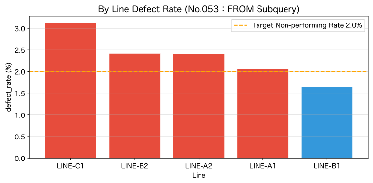
Reading the results

LINE-C1 (welding) has a target defect rate of 2.5%, but you can check whether the actual defect rate exceeds that
LINE-B1 (Assembly Line 1) is a priority candidate for process improvement if it achieves a high performance relative to the target of 1.5%.
FROM subqueries can be used as alternatives to HAVING sentence, but since they assign names (aliases) to intermediate tables, they improve readability for complex queries.

No.054: Using Subqueries with SELECT Phrases

Meaning in Practice

When you place a subquery in the SELECT clause, you can add a comparison table with the “overall average” or “benchmark value” to each row.
You can create it with a single SQL setup. You can see in a list whether this line is higher or lower than the overall average.

Approach to Analysis and Modeling

\text{Defect rate per line} - \underbrace{\text{Overall average defect rate}}_{\text{Added by SELECT clause subquery}} = \text{Deviation amount}

The SELECT clause subquery must return 1 rows 1 Column (scalar value).
This method is effective when you want to add the same constant (overall average) to all rows.

Check with Python

print("=== No.054 SELECTUsing subqueries in phrases ===\n")

# (1) Display the defect rate and overall average side by side for each line
print("① Defect Rates by Line vs overall average")
df54a = q(
    conn,
    """
SELECT
  line_code,
  ROUND(SUM(defect_qty) * 100.0 / SUM(production_qty), 2) AS line_dr,
  ROUND(
    (SELECT SUM(defect_qty) * 100.0 / SUM(production_qty)
     FROM production_daily),
  2) AS total_avg_dr
FROM production_daily
GROUP BY line_code
ORDER BY line_dr DESC
""",
)

# (2) Also calculate the difference (deviation) from the overall average
print("\n② The difference from the overall average (positive = Above average)")
df54b = q(
    conn,
    """
SELECT
  line_code,
  ROUND(SUM(defect_qty) * 100.0 / SUM(production_qty), 2) AS line_dr,
  ROUND(
    (SELECT SUM(defect_qty) * 100.0 / SUM(production_qty)
     FROM production_daily),
  2) AS total_avg_dr,
  ROUND(
    SUM(defect_qty) * 100.0 / SUM(production_qty)
    - (SELECT SUM(defect_qty) * 100.0 / SUM(production_qty)
       FROM production_daily),
  2) AS diff_from_avg
FROM production_daily
GROUP BY line_code
ORDER BY diff_from_avg DESC
""",
)

=== No.054 Using Subqueries with SELECT Phrases ===

(1) Defect Rate by Line vs. Overall Average
── SQL ─────────────────────────────────────────
  SELECT
    line_code,
    ROUND(SUM(defect_qty) * 100.0 / SUM(production_qty), 2) AS line_dr,
    ROUND(
      (SELECT SUM(defect_qty) * 100.0 / SUM(production_qty)
       FROM production_daily),
    2) AS total_avg_dr
  FROM production_daily
  GROUP BY line_code
  ORDER BY line_dr DESC
───────────────────────────────────────────────
shape: (5, 3)
┌───────────┬─────────┬──────────────┐
│ line_code ┆ line_dr ┆ total_avg_dr │
│ ---       ┆ ---     ┆ ---          │
│ str       ┆ f64     ┆ f64          │
╞═══════════╪═════════╪══════════════╡
│ LINE-C1   ┆ 3.13    ┆ 2.14         │
│ LINE-B2   ┆ 2.42    ┆ 2.14         │
│ LINE-A2   ┆ 2.41    ┆ 2.14         │
│ LINE-A1   ┆ 2.06    ┆ 2.14         │
│ LINE-B1   ┆ 1.65    ┆ 2.14         │
└───────────┴─────────┴──────────────┘
↳ Obtained in 5 rows

(2) Difference from the overall average (positive = above average)
── SQL ─────────────────────────────────────────
  SELECT
    line_code,
    ROUND(SUM(defect_qty) * 100.0 / SUM(production_qty), 2) AS line_dr,
    ROUND(
      (SELECT SUM(defect_qty) * 100.0 / SUM(production_qty)
       FROM production_daily),
    2) AS total_avg_dr,
    ROUND(
      SUM(defect_qty) * 100.0 / SUM(production_qty)
      - (SELECT SUM(defect_qty) * 100.0 / SUM(production_qty)
         FROM production_daily),
    2) AS diff_from_avg
  FROM production_daily
  GROUP BY line_code
  ORDER BY diff_from_avg DESC
───────────────────────────────────────────────
shape: (5, 4)
┌───────────┬─────────┬──────────────┬───────────────┐
│ line_code ┆ line_dr ┆ total_avg_dr ┆ diff_from_avg │
│ ---       ┆ ---     ┆ ---          ┆ ---           │
│ str       ┆ f64     ┆ f64          ┆ f64           │
╞═══════════╪═════════╪══════════════╪═══════════════╡
│ LINE-C1   ┆ 3.13    ┆ 2.14         ┆ 0.99          │
│ LINE-B2   ┆ 2.42    ┆ 2.14         ┆ 0.28          │
│ LINE-A2   ┆ 2.41    ┆ 2.14         ┆ 0.27          │
│ LINE-A1   ┆ 2.06    ┆ 2.14         ┆ -0.08         │
│ LINE-B1   ┆ 1.65    ┆ 2.14         ┆ -0.49         │
└───────────┴─────────┴──────────────┴───────────────┘
↳ Obtained in 5 rows

Reading the results

A line with a positive diff_from_avg indicates a higher defect rate than the overall average and is a priority for quality improvement.
The SELECT clause subquery adds the same scalar value to all lines, so it can be used as a Benchmark Comparison Table
By using ROUND() to align the decimal place to two decimal places, it can also be used as a report document as is.

No.055: Creating Subqueries Using IN

Meaning in Practice

IN (Subquery) When you use, you can acquire production data only for lines with maintenance records, such as
Dynamically narrow down records that match the conditions of a different table possible.

Approach to Analysis and Modeling

WHERE line_code IN (
  SELECT DISTINCT line_code FROM maintenance_log
)

This can also yield the same result with JOIN, but IN + subquery is:

Intuitively read the intent of the conditions
Dynamically generate a list of values returned by subqueries.

These are its characteristics. Conversely, using NOT IN allows you to extract lines that have not undergone maintenance.

Note: If NULL is included in the comparison list, NOT IN will be completely excluded,
It is safer to use NOT EXISTS for columns that may contain NULL (→ No.056).

Check with Python

print("=== No.055 INCreate a subquery using ===\n")

# (1) Production summary of lines with maintenance records
print("① Production summary of the maintenance line (IN）")
df55a = q(
    conn,
    """
SELECT
  line_code,
  COUNT(*)            AS work_days,
  SUM(production_qty) AS total_prod,
  SUM(defect_qty)     AS total_defect
FROM production_daily
WHERE line_code IN (
  SELECT DISTINCT line_code FROM maintenance_log
)
GROUP BY line_code
ORDER BY total_prod DESC
""",
)

# (2) Check lines not yet maintained (NOT IN)
print("\n② Checking lines not yet maintained (NOT IN）")
df55b = q(
    conn,
    """
SELECT line_code, line_name
FROM line_master
WHERE line_code NOT IN (
  SELECT DISTINCT line_code FROM maintenance_log
)
""",
)
if len(df55b) == 0:
    print("→ Maintenance records are available on all production lines (0Item)")

=== Creating Subqueries Using No.055 IN ===

(1) Production Summary (IN) of the Line Undergoing Maintenance
── SQL ─────────────────────────────────────────
  SELECT
    line_code,
    COUNT(*)            AS work_days,
    SUM(production_qty) AS total_prod,
    SUM(defect_qty)     AS total_defect
  FROM production_daily
  WHERE line_code IN (
    SELECT DISTINCT line_code FROM maintenance_log
  )
  GROUP BY line_code
  ORDER BY total_prod DESC
───────────────────────────────────────────────
shape: (5, 4)
┌───────────┬───────────┬────────────┬──────────────┐
│ line_code ┆ work_days ┆ total_prod ┆ total_defect │
│ ---       ┆ ---       ┆ ---        ┆ ---          │
│ str       ┆ i64       ┆ i64        ┆ i64          │
╞═══════════╪═══════════╪════════════╪══════════════╡
│ LINE-A1   ┆ 61        ┆ 28007      ┆ 576          │
│ LINE-B1   ┆ 61        ┆ 23146      ┆ 381          │
│ LINE-A2   ┆ 61        ┆ 13341      ┆ 321          │
│ LINE-B2   ┆ 61        ┆ 10624      ┆ 257          │
│ LINE-C1   ┆ 61        ┆ 7008       ┆ 219          │
└───────────┴───────────┴────────────┴──────────────┘
↳ Obtained in 5 rows

(2) Check lines not yet maintained (NOT IN)
── SQL ─────────────────────────────────────────
  SELECT line_code, line_name
  FROM line_master
  WHERE line_code NOT IN (
    SELECT DISTINCT line_code FROM maintenance_log
  )
───────────────────────────────────────────────
shape: (0, 2)
┌───────────┬───────────┐
│ line_code ┆ line_name │
│ ---       ┆ ---       │
│ null      ┆ null      │
╞═══════════╪═══════════╡
└───────────┴───────────┘
↳ 0 lines obtained
→ Maintenance records on all lines (0 entries)

Reading the results

Since maintenance records are available for all five lines, (1) serves as a production summary for all lines
In actual operations, it is often used to extract lines that have not undergone maintenance using NOT IN and create recommended inspection lists.
IN (Subquery) generates Dynamic List and automatically follows the addition or removal of the master

No.056: Creating Subqueries Using EXISTS

Meaning in Practice

EXISTS checks whether there is a record corresponding to the opponent’s table.
The question of “extracting production records from the day maintenance was performed”
You can match the date and line codes of production_daily and maintenance_log to answer.

Approach to Analysis and Modeling

WHERE EXISTS (
  SELECT 1
  FROM maintenance_log m
  WHERE m.line_code = p.line_code    -- Matching the outer line
    AND m.maint_date = p.prod_date   -- Same date
)

EXISTS only performs Line presence check, and since retrieving values is unnecessary, SELECT 1 is sufficient.
Differences from IN:

Comparison	IN	EXISTS
NULL Security	△ (NOT IN means dangerous)	○ (Do not bring NULL)
Conditions for Bonding with the Outer Table	single row	Multiple columns (combined condition)
Suitable Uses	Matching with the Value List	Verification of the existence of related records

Check with Python

print("=== No.056 EXISTSCreate a subquery using ===\n")

# (1) Consistency between maintenance implementation dates and production performance
print("① Production performance on the day maintenance was performed (EXISTS）")
df56a = q(
    conn,
    """
SELECT p.prod_date, p.line_code, p.production_qty, p.defect_qty
FROM production_daily p
WHERE EXISTS (
  SELECT 1
  FROM maintenance_log m
  WHERE m.line_code = p.line_code
    AND m.maint_date = p.prod_date
)
ORDER BY p.prod_date, p.line_code
LIMIT 15
""",
)

# (2) By line: Aggregation of maintenance days
print("\n② By Line Number of maintenance days (EXISTS + GROUP BY）")
df56b = q(
    conn,
    """
SELECT
  p.line_code,
  COUNT(*) AS maint_days,
  ROUND(AVG(p.defect_qty * 100.0 / p.production_qty), 2) AS avg_dr_on_maint_day
FROM production_daily p
WHERE EXISTS (
  SELECT 1
  FROM maintenance_log m
  WHERE m.line_code = p.line_code
    AND m.maint_date = p.prod_date
)
GROUP BY p.line_code
ORDER BY maint_days DESC
""",
)

=== No.056 Creating Subqueries Using EXISTS ===

(1) Production Results (EXISTS) on the Maintenance Implementation Date
── SQL ─────────────────────────────────────────
  SELECT p.prod_date, p.line_code, p.production_qty, p.defect_qty
  FROM production_daily p
  WHERE EXISTS (
    SELECT 1
    FROM maintenance_log m
    WHERE m.line_code = p.line_code
      AND m.maint_date = p.prod_date
  )
  ORDER BY p.prod_date, p.line_code
  LIMIT 15
───────────────────────────────────────────────
shape: (15, 4)
┌────────────┬───────────┬────────────────┬────────────┐
│ prod_date  ┆ line_code ┆ production_qty ┆ defect_qty │
│ ---        ┆ ---       ┆ ---            ┆ ---        │
│ str        ┆ str       ┆ i64            ┆ i64        │
╞════════════╪═══════════╪════════════════╪════════════╡
│ 2025-01-06 ┆ LINE-A1   ┆ 471            ┆ 9          │
│ 2025-01-13 ┆ LINE-A1   ┆ 467            ┆ 8          │
│ 2025-01-17 ┆ LINE-C1   ┆ 115            ┆ 3          │
│ 2025-01-21 ┆ LINE-B2   ┆ 174            ┆ 3          │
│ 2025-01-23 ┆ LINE-A1   ┆ 424            ┆ 9          │
│ …          ┆ …         ┆ …              ┆ …          │
│ 2025-02-18 ┆ LINE-C1   ┆ 116            ┆ 4          │
│ 2025-02-19 ┆ LINE-A2   ┆ 210            ┆ 8          │
│ 2025-02-21 ┆ LINE-A2   ┆ 222            ┆ 4          │
│ 2025-02-21 ┆ LINE-B1   ┆ 371            ┆ 7          │
│ 2025-02-24 ┆ LINE-B2   ┆ 174            ┆ 4          │
└────────────┴───────────┴────────────────┴────────────┘
↳ Obtained in 15 rows

(2) Number of maintenance days per line (EXISTS + GROUP BY)
── SQL ─────────────────────────────────────────
  SELECT
    p.line_code,
    COUNT(*) AS maint_days,
    ROUND(AVG(p.defect_qty * 100.0 / p.production_qty), 2) AS avg_dr_on_maint_day
  FROM production_daily p
  WHERE EXISTS (
    SELECT 1
    FROM maintenance_log m
    WHERE m.line_code = p.line_code
      AND m.maint_date = p.prod_date
  )
  GROUP BY p.line_code
  ORDER BY maint_days DESC
───────────────────────────────────────────────
shape: (5, 3)
┌───────────┬────────────┬─────────────────────┐
│ line_code ┆ maint_days ┆ avg_dr_on_maint_day │
│ ---       ┆ ---        ┆ ---                 │
│ str       ┆ i64        ┆ f64                 │
╞═══════════╪════════════╪═════════════════════╡
│ LINE-C1   ┆ 8          ┆ 3.08                │
│ LINE-B2   ┆ 5          ┆ 2.1                 │
│ LINE-A2   ┆ 5          ┆ 2.74                │
│ LINE-A1   ┆ 5          ┆ 2.07                │
│ LINE-B1   ┆ 4          ┆ 1.79                │
└───────────┴────────────┴─────────────────────┘
↳ Obtained in 5 rows

Reading the results

Maintenance dates are usually Downtime occurred, leading to reduced production volume.,
The impact on defect rates (improvement or deterioration) varies depending on equipment condition
By comparing the avg_dr_on_maint_day (average defect rate on maintenance days) with days when maintenance was not performed,
Can be used for “measuring maintenance effectiveness”
If LINE-C1 has the highest maintenance days, it suggests aging welding equipment and high adjustment frequency.

No.057: Understanding Correlation Subqueries

Meaning in Practice

Correlation Subquery is a structure where the inner query is reexecuted every time each row of the outer query is processed.
You can answer the question: “How do you identify the day when the Average of your own line of each line is exceeded?”

This enables Line-specific anomaly detection that cannot be achieved by comparing it to the “overall average” (No.052).

Approach to Analysis and Modeling

WHERE p.defect_qty > (
  SELECT AVG(defect_qty)
  FROM production_daily p2
  WHERE p2.line_code = p.line_code   -- ← Evaluation linked to the outer line
)

How it works:

When an outer query processes the first line of LINE-A1, the inner query calculates the average number of defects in LINE-A1.
For the LINE-A2 line, calculate the average of the LINE-A2 inside

This is how The inner side changes in sync with the outer value. is characteristic of correlation subqueries.

Note: In large tables, subqueries are executed row-by-row, so performance needs to be monitored.
In practice, consider rewriting it in window function (Chapter 7).

Check with Python

print("=== No.057 Understanding Correlation Subqueries ===\n")

# (1) Days when the average number of defects per line exceeds (correlation subquery)
print("① Days exceeding the average number of defects by line (top 15 Item)")
df57a = q(
    conn,
    """
SELECT
  p.line_code,
  p.prod_date,
  p.defect_qty,
  ROUND(
    (SELECT AVG(defect_qty) FROM production_daily p2
     WHERE p2.line_code = p.line_code),
  1) AS line_avg_defect
FROM production_daily p
WHERE p.defect_qty > (
  SELECT AVG(defect_qty)
  FROM production_daily p2
  WHERE p2.line_code = p.line_code
)
ORDER BY p.line_code, p.defect_qty DESC
LIMIT 15
""",
)

# (2) By line: Aggregation of days exceeding the average
print("\n② By Line Number of days exceeding average defects")
df57b = q(
    conn,
    """
SELECT
  p.line_code,
  COUNT(*) AS above_avg_days
FROM production_daily p
WHERE p.defect_qty > (
  SELECT AVG(defect_qty)
  FROM production_daily p2
  WHERE p2.line_code = p.line_code
)
GROUP BY p.line_code
ORDER BY above_avg_days DESC
""",
)

# visualization
fig, ax = plt.subplots(figsize=(8, 4))
ax.barh(df57b["line_code"].to_list(), df57b["above_avg_days"].to_list(), color="#e67e22", edgecolor="white")
ax.set_title("By Line Number of days exceeding the average number of defects in your own line (No.057: Correlation Subquery)", fontsize=12)
ax.set_xlabel("number_of_days")
ax.set_ylabel("Line")
ax.grid(axis="x", alpha=0.4)
plt.tight_layout()
plt.show()

=== No.057 Understanding Correlation Subqueries ===

(1) Days exceeding the average number of defects per line (top 15 cases)
── SQL ─────────────────────────────────────────
  SELECT
    p.line_code,
    p.prod_date,
    p.defect_qty,
    ROUND(
      (SELECT AVG(defect_qty) FROM production_daily p2
       WHERE p2.line_code = p.line_code),
    1) AS line_avg_defect
  FROM production_daily p
  WHERE p.defect_qty > (
    SELECT AVG(defect_qty)
    FROM production_daily p2
    WHERE p2.line_code = p.line_code
  )
  ORDER BY p.line_code, p.defect_qty DESC
  LIMIT 15
───────────────────────────────────────────────
shape: (15, 4)
┌───────────┬────────────┬────────────┬─────────────────┐
│ line_code ┆ prod_date  ┆ defect_qty ┆ line_avg_defect │
│ ---       ┆ ---        ┆ ---        ┆ ---             │
│ str       ┆ str        ┆ i64        ┆ f64             │
╞═══════════╪════════════╪════════════╪═════════════════╡
│ LINE-A1   ┆ 2025-03-05 ┆ 15         ┆ 9.4             │
│ LINE-A1   ┆ 2025-03-17 ┆ 15         ┆ 9.4             │
│ LINE-A1   ┆ 2025-03-25 ┆ 15         ┆ 9.4             │
│ LINE-A1   ┆ 2025-01-09 ┆ 14         ┆ 9.4             │
│ LINE-A1   ┆ 2025-01-15 ┆ 14         ┆ 9.4             │
│ …         ┆ …          ┆ …          ┆ …               │
│ LINE-A1   ┆ 2025-03-14 ┆ 13         ┆ 9.4             │
│ LINE-A1   ┆ 2025-01-17 ┆ 12         ┆ 9.4             │
│ LINE-A1   ┆ 2025-02-18 ┆ 12         ┆ 9.4             │
│ LINE-A1   ┆ 2025-03-10 ┆ 12         ┆ 9.4             │
│ LINE-A1   ┆ 2025-01-28 ┆ 11         ┆ 9.4             │
└───────────┴────────────┴────────────┴─────────────────┘
↳ Obtained in 15 rows

(2) Number of days exceeding average defect count by line
── SQL ─────────────────────────────────────────
  SELECT
    p.line_code,
    COUNT(*) AS above_avg_days
  FROM production_daily p
  WHERE p.defect_qty > (
    SELECT AVG(defect_qty)
    FROM production_daily p2
    WHERE p2.line_code = p.line_code
  )
  GROUP BY p.line_code
  ORDER BY above_avg_days DESC
───────────────────────────────────────────────
shape: (5, 2)
┌───────────┬────────────────┐
│ line_code ┆ above_avg_days │
│ ---       ┆ ---            │
│ str       ┆ i64            │
╞═══════════╪════════════════╡
│ LINE-C1   ┆ 29             │
│ LINE-B1   ┆ 27             │
│ LINE-A2   ┆ 27             │
│ LINE-A1   ┆ 27             │
│ LINE-B2   ┆ 23             │
└───────────┴────────────────┘
↳ Obtained in 5 rows

svg

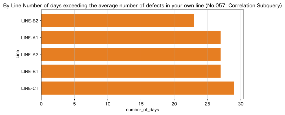
Reading the results

Correlation subqueries can identify abnormal days using The “Own Line-Specific Average” for Each Line as a threshold
It is statistically natural (distributed near median) that about half of the operating days on any line exceed the average of their own lines.
In practice, adding additional conditions such as “three consecutive days or more, above average” allows for designing more accurate alerts

No.058: Creating CTEs with WITH Phrases

Meaning in Practice

CTE（Common Table Expression） is a named temporary table defined by WITH sentence.
The process of “calculating the monthly defect rate once and then comparing it further”
You can write subqueries in Structure that allows reading from top to bottom without nesting multiple times.

Approach to Analysis and Modeling

WITH monthly_dr AS (          -- ← CTE Definition
  SELECT strftime('%Y-%m', prod_date) AS ym,
         line_code,
         SUM(defect_qty)*100.0/SUM(production_qty) AS defect_rate
  FROM production_daily
  GROUP BY ym, line_code
)
SELECT * FROM monthly_dr      -- ← CTE Reference as a regular table
ORDER BY ym, line_code

CTE is evaluated at runtime and also has the advantage of Multiple references within a query (via DBMS).
The results are the same as using subqueries, but readability and maintainability are greatly improved.

Check with Python

print("=== No.058 WITHin a haikuCTEmake ===\n")

# (1) Define and retrieve the monthly defect rate table in CTE
print("① CTE:Monthly Non-Defect Rate Table (monthly_dr）")
df58a = q(
    conn,
    """
WITH monthly_dr AS (
  SELECT
    strftime('%Y-%m', prod_date) AS ym,
    line_code,
    SUM(production_qty)  AS total_prod,
    SUM(defect_qty)      AS total_defect,
    ROUND(SUM(defect_qty) * 100.0 / SUM(production_qty), 2) AS defect_rate
  FROM production_daily
  GROUP BY ym, line_code
)
SELECT *
FROM monthly_dr
ORDER BY ym, line_code
""",
)

# (2) Extract the highest defect rate line for each month by referencing CTE
print("\n② The defect rate is at the highest monthly limit (CTE References + Scala Subquery)")
df58b = q(
    conn,
    """
WITH monthly_dr AS (
  SELECT
    strftime('%Y-%m', prod_date) AS ym,
    line_code,
    ROUND(SUM(defect_qty) * 100.0 / SUM(production_qty), 2) AS defect_rate
  FROM production_daily
  GROUP BY ym, line_code
)
SELECT ym, line_code, defect_rate
FROM monthly_dr
WHERE defect_rate = (
  SELECT MAX(defect_rate) FROM monthly_dr AS sub
  WHERE sub.ym = monthly_dr.ym
)
ORDER BY ym
""",
)

=== No.058 Creating CTEs with WITH Phrases ===

(1) CTE: Monthly Defect Rate Table (monthly_dr)
── SQL ─────────────────────────────────────────
  WITH monthly_dr AS (
    SELECT
      strftime('%Y-%m', prod_date) AS ym,
      line_code,
      SUM(production_qty)  AS total_prod,
      SUM(defect_qty)      AS total_defect,
      ROUND(SUM(defect_qty) * 100.0 / SUM(production_qty), 2) AS defect_rate
    FROM production_daily
    GROUP BY ym, line_code
  )
  SELECT *
  FROM monthly_dr
  ORDER BY ym, line_code
───────────────────────────────────────────────
shape: (15, 5)
┌─────────┬───────────┬────────────┬──────────────┬─────────────┐
│ ym      ┆ line_code ┆ total_prod ┆ total_defect ┆ defect_rate │
│ ---     ┆ ---       ┆ ---        ┆ ---          ┆ ---         │
│ str     ┆ str       ┆ i64        ┆ i64          ┆ f64         │
╞═════════╪═══════════╪════════════╪══════════════╪═════════════╡
│ 2025-01 ┆ LINE-A1   ┆ 9107       ┆ 192          ┆ 2.11        │
│ 2025-01 ┆ LINE-A2   ┆ 4366       ┆ 95           ┆ 2.18        │
│ 2025-01 ┆ LINE-B1   ┆ 7512       ┆ 138          ┆ 1.84        │
│ 2025-01 ┆ LINE-B2   ┆ 3497       ┆ 91           ┆ 2.6         │
│ 2025-01 ┆ LINE-C1   ┆ 2277       ┆ 67           ┆ 2.94        │
│ …       ┆ …         ┆ …          ┆ …            ┆ …           │
│ 2025-03 ┆ LINE-A1   ┆ 9751       ┆ 191          ┆ 1.96        │
│ 2025-03 ┆ LINE-A2   ┆ 4541       ┆ 117          ┆ 2.58        │
│ 2025-03 ┆ LINE-B1   ┆ 7995       ┆ 127          ┆ 1.59        │
│ 2025-03 ┆ LINE-B2   ┆ 3623       ┆ 80           ┆ 2.21        │
│ 2025-03 ┆ LINE-C1   ┆ 2406       ┆ 73           ┆ 3.03        │
└─────────┴───────────┴────────────┴──────────────┴─────────────┘
↳ Obtained in 15 rows

(2) The highest defect rate line per month (see CTE + Scalar subquery)
── SQL ─────────────────────────────────────────
  WITH monthly_dr AS (
    SELECT
      strftime('%Y-%m', prod_date) AS ym,
      line_code,
      ROUND(SUM(defect_qty) * 100.0 / SUM(production_qty), 2) AS defect_rate
    FROM production_daily
    GROUP BY ym, line_code
  )
  SELECT ym, line_code, defect_rate
  FROM monthly_dr
  WHERE defect_rate = (
    SELECT MAX(defect_rate) FROM monthly_dr AS sub
    WHERE sub.ym = monthly_dr.ym
  )
  ORDER BY ym
───────────────────────────────────────────────
shape: (3, 3)
┌─────────┬───────────┬─────────────┐
│ ym      ┆ line_code ┆ defect_rate │
│ ---     ┆ ---       ┆ ---         │
│ str     ┆ str       ┆ f64         │
╞═════════╪═══════════╪═════════════╡
│ 2025-01 ┆ LINE-C1   ┆ 2.94        │
│ 2025-02 ┆ LINE-C1   ┆ 3.4         │
│ 2025-03 ┆ LINE-C1   ┆ 3.03        │
└─────────┴───────────┴─────────────┘
↳ Retrieved in 3 lines

Reading the results

By defining the CTE monthly_dr, you can All in one place monthly aggregation logic
In (2), CTEs are referenced multiple times (outer SELECT and inner scalar subqueries), eliminating duplicate descriptions of the same logic
Monthly defect rate worst line information is an important KPI directly linked to setting improvement priorities for the following month

No.059: Organizing Complex Aggregations Using CTE

Meaning in Practice

The monthly KPI report aggregates ‘monthly and line production volume, defect rate, and loss costs’ all at once.
You are required to submit it to management. By stacking multiple CTEs,
Excel Processing equivalent to multiple sheets can be completed with a single SQL file.

Approach to Analysis and Modeling

[CTE 1: monthly] Daily → Monthly Summary
        ↓
[CTE 2: with_loss] Monthly Aggregation × line_master → Loss Cost Conversion
        ↓
[Final SELECT] Report Output

Each CTE can be processed by referencing the previous CTE,
Data Pipeline can be represented within SQL.

Check with Python

print("=== No.059 CTEOrganize complex aggregations using ===\n")

# (1) Multiple CTEs: Monthly KPI dashboard
print("① multipleCTE: List of monthly loss costs")
df59 = q(
    conn,
    """
WITH
monthly AS (
  SELECT
    strftime('%Y-%m', prod_date) AS ym,
    line_code,
    SUM(production_qty)  AS total_prod,
    SUM(defect_qty)      AS total_defect
  FROM production_daily
  GROUP BY ym, line_code
),
with_loss AS (
  SELECT
    m.ym,
    m.line_code,
    m.total_prod,
    m.total_defect,
    ROUND(m.total_defect * 100.0 / m.total_prod, 2) AS defect_rate,
    m.total_defect * l.unit_cost AS loss_cost
  FROM monthly m
  JOIN line_master l ON m.line_code = l.line_code
)
SELECT *
FROM with_loss
ORDER BY ym, loss_cost DESC
""",
)

# Visualization: Monthly loss cost (stacked bar graph by line)
LINES_ORDER = ["LINE-A1", "LINE-A2", "LINE-B1", "LINE-B2", "LINE-C1"]
COLORS_59 = ["#3498db", "#e74c3c", "#2ecc71", "#f39c12", "#9b59b6"]
YMS = sorted(df59["ym"].unique().to_list())

fig, ax = plt.subplots(figsize=(9, 5))
bottoms = [0] * len(YMS)
for i, lc in enumerate(LINES_ORDER):
    sub = df59.filter(pl.col("line_code") == lc).sort("ym")
    ym_set = sub["ym"].to_list()
    costs = [int(sub.filter(pl.col("ym") == ym)["loss_cost"][0]) if ym in ym_set else 0 for ym in YMS]
    ax.bar(YMS, costs, bottom=bottoms, color=COLORS_59[i], label=lc, edgecolor="white", linewidth=0.5)
    bottoms = [b + c for b, c in zip(bottoms, costs)]

ax.set_title("monthly Non-performing loss cost (No.059: pluralCTE）", fontsize=13)
ax.set_xlabel("Year and month")
ax.set_ylabel("Loss cost (yen)")
ax.legend(loc="upper right", fontsize=9)
ax.grid(axis="y", alpha=0.4)
plt.tight_layout()
plt.show()

=== No.059 Organizing Complex Aggregations Using CTE ===

(1) Multiple CTEs: List of monthly loss costs
── SQL ─────────────────────────────────────────
  WITH
  monthly AS (
    SELECT
      strftime('%Y-%m', prod_date) AS ym,
      line_code,
      SUM(production_qty)  AS total_prod,
      SUM(defect_qty)      AS total_defect
    FROM production_daily
    GROUP BY ym, line_code
  ),
  with_loss AS (
    SELECT
      m.ym,
      m.line_code,
      m.total_prod,
      m.total_defect,
      ROUND(m.total_defect * 100.0 / m.total_prod, 2) AS defect_rate,
      m.total_defect * l.unit_cost AS loss_cost
    FROM monthly m
    JOIN line_master l ON m.line_code = l.line_code
  )
  SELECT *
  FROM with_loss
  ORDER BY ym, loss_cost DESC
───────────────────────────────────────────────
shape: (15, 6)
┌─────────┬───────────┬────────────┬──────────────┬─────────────┬───────────┐
│ ym      ┆ line_code ┆ total_prod ┆ total_defect ┆ defect_rate ┆ loss_cost │
│ ---     ┆ ---       ┆ ---        ┆ ---          ┆ ---         ┆ ---       │
│ str     ┆ str       ┆ i64        ┆ i64          ┆ f64         ┆ i64       │
╞═════════╪═══════════╪════════════╪══════════════╪═════════════╪═══════════╡
│ 2025-01 ┆ LINE-A2   ┆ 4366       ┆ 95           ┆ 2.18        ┆ 807500    │
│ 2025-01 ┆ LINE-C1   ┆ 2277       ┆ 67           ┆ 2.94        ┆ 455600    │
│ 2025-01 ┆ LINE-B2   ┆ 3497       ┆ 91           ┆ 2.6         ┆ 382200    │
│ 2025-01 ┆ LINE-A1   ┆ 9107       ┆ 192          ┆ 2.11        ┆ 230400    │
│ 2025-01 ┆ LINE-B1   ┆ 7512       ┆ 138          ┆ 1.84        ┆ 131100    │
│ …       ┆ …         ┆ …          ┆ …            ┆ …           ┆ …         │
│ 2025-03 ┆ LINE-A2   ┆ 4541       ┆ 117          ┆ 2.58        ┆ 994500    │
│ 2025-03 ┆ LINE-C1   ┆ 2406       ┆ 73           ┆ 3.03        ┆ 496400    │
│ 2025-03 ┆ LINE-B2   ┆ 3623       ┆ 80           ┆ 2.21        ┆ 336000    │
│ 2025-03 ┆ LINE-A1   ┆ 9751       ┆ 191          ┆ 1.96        ┆ 229200    │
│ 2025-03 ┆ LINE-B1   ┆ 7995       ┆ 127          ┆ 1.59        ┆ 120650    │
└─────────┴───────────┴────────────┴──────────────┴─────────────┴───────────┘
↳ Obtained in 15 rows

svg

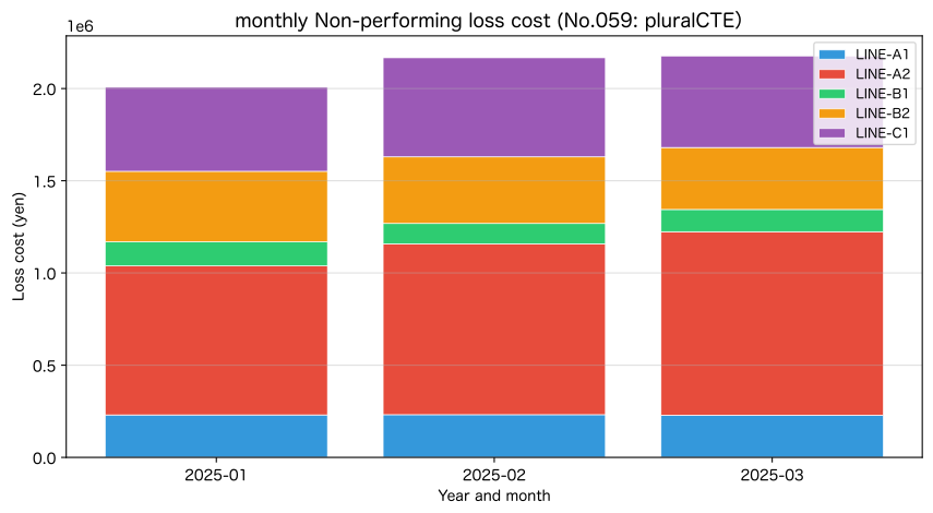
Reading the results

Instantly see Composition of monthly loss costs on stacked bar graphs
The LINE-A2 (crankshaft) has a high unit_cost of 8,500 yen, so even with fewer defects, the impact on loss costs is significant.
Using multiple CTEs makes it easier to independently verify and debug intermediate steps (monthly)
→ Directly reduces query maintenance workload for quality control dashboards

No.060: Creating a temporary analysis table

Meaning in Practice

The monthly quality management report includes “production performance, defect rate, loss costs, maintenance performance, and status assessments for all lines.”
You are required to submit them all together on a single table.
By stacking CTEs in multiple layers, you can generate such Comprehensive dashboard table directly from SQL.

Approach to Analysis and Modeling

[CTE 1: prod_summary] Production Aggregation by Line (Number of Operating Days, Total Production, Defect Rate)
        ↓
[CTE 2: maint_summary] Maintenance Summary by Line (Number of Cases & Downtime)
        ↓
[CTE 3: dashboard]       JOIN + status check (CASE formula)
        ↓
[Final SELECT] Report Output

Status Determination Logic:

\text{status} = \begin{cases} \text{To improve} & \text{if } \text{defect\_rate} > \text{target\_dr} \times 1.2 \\ \text{Note} & \text{if} \text{defect\_rate} > \text{target\_dr} \\ \text{normal} & \text{otherwise} \end{cases}

Check with Python

print("=== No.060 Create a temporary analysis table ===\n")

# (1) CTE Multi-Stage: Comprehensive Analysis Dashboard
print("① CTEComprehensive Analysis Dashboard")
df60 = q(
    conn,
    """
WITH
prod_summary AS (
  SELECT
    line_code,
    COUNT(DISTINCT prod_date) AS work_days,
    SUM(production_qty)       AS total_prod,
    SUM(defect_qty)           AS total_defect,
    ROUND(SUM(defect_qty) * 100.0 / SUM(production_qty), 2) AS defect_rate
  FROM production_daily
  GROUP BY line_code
),
maint_summary AS (
  SELECT
    line_code,
    COUNT(*)                      AS maint_count,
    ROUND(SUM(downtime_hours), 1) AS total_downtime
  FROM maintenance_log
  GROUP BY line_code
),
dashboard AS (
  SELECT
    p.line_code,
    l.line_name,
    l.section,
    p.work_days,
    p.total_prod,
    p.defect_rate,
    ROUND(l.target_dr * 100, 1)       AS target_dr_pct,
    COALESCE(m.maint_count,    0)     AS maint_count,
    COALESCE(m.total_downtime, 0)     AS total_downtime,
    p.total_defect * l.unit_cost      AS total_loss,
    CASE
      WHEN p.defect_rate > l.target_dr * 100 * 1.2 THEN 'To improve'
      WHEN p.defect_rate > l.target_dr * 100       THEN 'Note'
      ELSE 'normal'
    END AS status
  FROM prod_summary p
  JOIN line_master l ON p.line_code = l.line_code
  LEFT JOIN maint_summary m ON p.line_code = m.line_code
)
SELECT * FROM dashboard ORDER BY defect_rate DESC
""",
)

# Visualization: Actual vs. Target Defect Rate (Group Bar Graph)
LINES_60 = df60["line_code"].to_list()
ACTUAL_DR = df60["defect_rate"].to_list()
TARGET_DR = df60["target_dr_pct"].to_list()
STATUSES = df60["status"].to_list()
STATUS_COL = {"normal": "#2ecc71", "Note": "#f39c12", "To improve": "#e74c3c"}
BAR_COLORS = [STATUS_COL[s] for s in STATUSES]

x = np.arange(len(LINES_60))
width = 0.35
fig, ax = plt.subplots(figsize=(9, 5))
ax.bar(x - width / 2, ACTUAL_DR, width, color=BAR_COLORS, label="Performance Defect Rate", edgecolor="white")
ax.bar(x + width / 2, TARGET_DR, width, color="#95a5a6", label="Target Non-performing Rate", edgecolor="white")
ax.set_title("By Line Performance Defect Rate vs Target Non-performing Rate (No.060：CTE Comprehensive dashboard)", fontsize=12)
ax.set_xlabel("Line")
ax.set_ylabel("defect_rate (%)")
ax.set_xticks(x)
ax.set_xticklabels(LINES_60)
ax.legend(fontsize=10)
ax.grid(axis="y", alpha=0.4)
plt.tight_layout()
plt.show()

=== No.060 Creating a Temporary Analysis Table ===

(1) Comprehensive Analysis Dashboard Using CTE
── SQL ─────────────────────────────────────────
  WITH
  prod_summary AS (
    SELECT
      line_code,
      COUNT(DISTINCT prod_date) AS work_days,
      SUM(production_qty)       AS total_prod,
      SUM(defect_qty)           AS total_defect,
      ROUND(SUM(defect_qty) * 100.0 / SUM(production_qty), 2) AS defect_rate
    FROM production_daily
    GROUP BY line_code
  ),
  maint_summary AS (
    SELECT
      line_code,
      COUNT(*)                      AS maint_count,
      ROUND(SUM(downtime_hours), 1) AS total_downtime
    FROM maintenance_log
    GROUP BY line_code
  ),
  dashboard AS (
    SELECT
      p.line_code,
      l.line_name,
      l.section,
      p.work_days,
      p.total_prod,
      p.defect_rate,
      ROUND(l.target_dr * 100, 1)       AS target_dr_pct,
      COALESCE(m.maint_count,    0)     AS maint_count,
      COALESCE(m.total_downtime, 0)     AS total_downtime,
      p.total_defect * l.unit_cost      AS total_loss,
      CASE
        WHEN p.defect_rate > l.target_dr * 100 * 1.2 THEN 'Need to Improve'
        WHEN p.defect_rate > l.target_dr * 100 THEN 'Be careful'
        ELSE 'normal'
      END AS status
    FROM prod_summary p
    JOIN line_master l ON p.line_code = l.line_code
    LEFT JOIN maint_summary m ON p.line_code = m.line_code
  )
  SELECT * FROM dashboard ORDER BY defect_rate DESC
───────────────────────────────────────────────
shape: (5, 11)
┌───────────┬────────────┬──────────┬───────────┬───┬────────────┬────────────┬───────────┬────────┐
│ line_code ┆ line_name  ┆ section  ┆ work_days ┆ … ┆ maint_coun ┆ total_down ┆ total_los ┆ status │
│ ---       ┆ ---        ┆ ---      ┆ ---       ┆   ┆ t          ┆ time       ┆ s         ┆ ---    │
│ str       ┆ str        ┆ str      ┆ i64       ┆   ┆ ---        ┆ ---        ┆ ---       ┆ str    │
│           ┆            ┆          ┆           ┆   ┆ i64        ┆ f64        ┆ i64       ┆        │
╞═══════════╪════════════╪══════════╪═══════════╪═══╪════════════╪════════════╪═══════════╪════════╡
│ LINE-C1   ┆ welding line ┆ welding     ┆ 61        ┆ … ┆ 8          ┆ 45.6       ┆ 1489200   ┆ To improve │
│           ┆ 1          ┆          ┆           ┆   ┆            ┆            ┆           ┆        │
│ LINE-B2   ┆ assembly line ┆ Assembly     ┆ 61        ┆ … ┆ 5          ┆ 29.1       ┆ 1079400   ┆ To improve │
│           ┆ 2          ┆          ┆           ┆   ┆            ┆            ┆           ┆        │
│ LINE-A2   ┆ Machining ┆ machining ┆ 61        ┆ … ┆ 5          ┆ 25.6       ┆ 2728500   ┆ To improve │
│           ┆ Inn2      ┆          ┆           ┆   ┆            ┆            ┆           ┆        │
│ LINE-A1   ┆ Machining ┆ machining ┆ 61        ┆ … ┆ 5          ┆ 19.8       ┆ 691200    ┆ Note │
│           ┆ Inn1      ┆          ┆           ┆   ┆            ┆            ┆           ┆        │
│ LINE-B1   ┆ assembly line ┆ Assembly     ┆ 61        ┆ … ┆ 4          ┆ 14.6       ┆ 361950    ┆ Note │
│           ┆ 1          ┆          ┆           ┆   ┆            ┆            ┆           ┆        │
└───────────┴────────────┴──────────┴───────────┴───┴────────────┴────────────┴───────────┴────────┘
↳ Obtained in 5 rows

svg

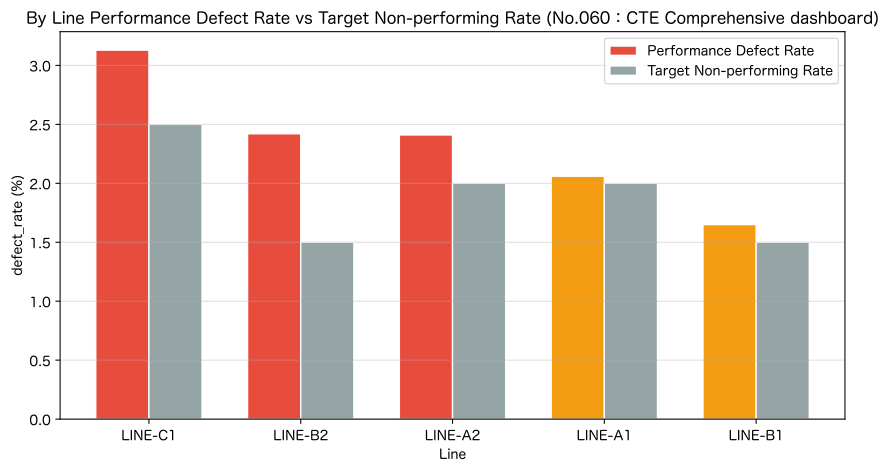
Reading the results

Achievements vs Objective comparison graph shows the quality status of each line at a glance.
total_loss (Total Loss Costs) can be used as a guideline for the “maximum amount of improvement investment.”
→ If you have ‘improvement investment costs < loss costs that can be reduced,’ you can justify your investment.
If LINE-C1 has a high defect rate despite having many maint_count,
It may be a sign that a “fundamental upgrade of the equipment” is needed.
This SQL dashboard is executed as a periodic batch and defined as a BITool View,
Enables reports that are automatically updated every month.

Practical Implications Seen Through Target Exercise

Distinguishing Between Subqueries and CTEs

Situation	Recommended Approach
I want to dynamically calculate the comparison criteria	Scala Subquery (WHERE Phrase)
Want to filter further after aggregation	FROM Subquery (Inline View)
I want to add benchmark values to each row	SELECT Phrase Subquery
Want to use dynamic thresholds for each line or group	Correlation Subquery
Want to organize multi-stage aggregation	CTE (WITH Sentence)
Want to reuse the same logic in multiple locations	CTE

Application patterns for manufacturing KPI aggregation

WITH Daily Aggregation AS (...)
   , Monthly Aggregation AS (Aggregated from Daily Aggregate)
   , Loss cost calculation AS (monthly aggregation × master)
   , Status Determination AS (Loss Cost × Threshold)
SELECT * FROM Status Check

If you design Quality KPI dashboard SQL with this pattern,
Automate monthly report creation with just one button.

What is necessary for practical implementation

1. Reviewing Table Design

The production_daily, line_master, and maintenance_log used in this exercise
We assume tables corresponding to actual Manufacturing Execution Systems (MES) and Quality Management Systems (QMS)
In actual implementation, Table normalization levels and date type unification (TEXT vs DATE type) is crucial

2. Consideration for Performance

Correlation subqueries have O(n²) Possibility of becoming if they have many lines.
For large tables, consider rewriting JOIN or utilizing window function (Chapter 7)

3. Integration with BI Tools

The CTE dashboard SQL designed here is used in BigQuery, Redshift, Snowflake, and other
Defined as Regular viewing (Materialized View） on cloud DWH,
Integration of data with Tableau / Power BI / Looker becomes easy.

4. Gradual Automation

Step 1: Manual query execution → Monthly report creation
Step 2: Organize queries with CTE → Maintain easy-to-maintain SQL
Step 3: Register views for DWHs → Auto-update
Step 4: BI Tool Integration → Self-Service Analysis

Conclusion

In this chapter, we put SQL’s applied features Subquery and CTE into practice with manufacturing quality control data.

No.	Acquired Skills	Practical Value
051	Scalar Subquery	Setting dynamic comparison criteria
052	WHERE Subquery	Detection of abnormal days above average
053	FROM Subquery	Post-aggregation filter (inline view)
054	SELECT Subquery	Calculation of Overall Average Addition and Deviation
055	IN Subquery	Filtering with dynamic lists
056	EXISTS	Presence Confirmation under Complex Conditions
057	Correlation Subquery	Abnormality detection using dynamic thresholds by line
058	CTE (WITH Sentence)	Organized by name in aggregation logic
059	Multiple CTE + JOIN	Building a Monthly KPI Dashboard
060	CTE Multi-stacking	Automatic generation of comprehensive analysis tables

Chapter 2 (Part 1)7Chapter) will teach window function (ROW_NUMBER, LAG, SUM OVER).
Learn how to describe “dynamic aggregation per row” more efficiently achieved with correlation subqueries.

Consultations for Corporations

Regarding Building a Data Analysis Platform, SQL Training and in-house production support, and KPI Dashboard Design in manufacturing,
Suri Kobo accepts consultations for corporate clients.

A system for automatically aggregating and visualizing quality data from manufacturing sites using SQL, as discussed in this exercise,
From implementation support to designing educational programs, please feel free to contact us.

📩 Contact Us: surikobo.co.jp/contact Please feel free to consult us first.

Automating abnormality detection and KPI aggregation on production lines with subqueries and CTE

Automating abnormality detection and KPI aggregation on production lines with subqueries and CTE

SQL 100 Exercise Chapter 6 (No.051–No.060): Subqueries and CTE

Introduction: Practical Challenges in Manufacturing Covered in This Article

Common situations on site

Why is this issue so difficult to judge?

Overview of Exercise covered this time

Preparing the Python environment

Creation of Fictional Data

No.051: Understanding the Basics of Subqueries

Meaning in Practice

Approach to Analysis and Modeling

Check with Python

Reading the results

No.052: Using Subqueries with WHERE Phrases

Meaning in Practice

Approach to Analysis and Modeling

Check with Python

Reading the results

No.053: Using Subqueries with FROM Phrases

Meaning in Practice

Approach to Analysis and Modeling

Check with Python

Reading the results

No.054: Using Subqueries with SELECT Phrases

Meaning in Practice

Approach to Analysis and Modeling

Check with Python

Reading the results

No.055: Creating Subqueries Using IN

Meaning in Practice

Approach to Analysis and Modeling

Check with Python

Reading the results

No.056: Creating Subqueries Using EXISTS

Meaning in Practice

Approach to Analysis and Modeling

Check with Python

Reading the results

No.057: Understanding Correlation Subqueries

Meaning in Practice

Approach to Analysis and Modeling

Check with Python

Reading the results

No.058: Creating CTEs with WITH Phrases

Meaning in Practice

Approach to Analysis and Modeling

Check with Python

Reading the results

No.059: Organizing Complex Aggregations Using CTE

Meaning in Practice

Approach to Analysis and Modeling

Check with Python

Reading the results

No.060: Creating a temporary analysis table

Meaning in Practice

Approach to Analysis and Modeling

Check with Python

Reading the results

Practical Implications Seen Through Target Exercise

Distinguishing Between Subqueries and CTEs

Application patterns for manufacturing KPI aggregation

What is necessary for practical implementation

1. Reviewing Table Design

2. Consideration for Performance

3. Integration with BI Tools

4. Gradual Automation

Conclusion

Consultations for Corporations

Related Posts

Integrating data quality management, SQL design, and BI integration into production line operations

Deepening manufacturing decision-making with SQL application analysis techniques

Automate order KPIs, customer analysis, and inventory risk assessment using SQL

Analyze monthly trends on manufacturing lines from multiple perspectives using SQL window functions

Perform cross-analysis of factory, parts, and inspection records using SQL JOINs