Integrating data quality management, SQL design, and BI integration into production line operations

SQL 100 Exercises Chapter 10 (No.091–No.100): Practical Operation, Performance, and Design

[!NOTE] This material is a notebook previously used by Sukari Kobo (or personally by the representative, Kazuyama), and has been restructured, edited, and published with the company’s permission. All data listed is fictional and has no relation whatsoever to real companies, factories, or figures.

Introduction: Practical Challenges in Manufacturing Covered in This Article

Chapter 10, the final chapter of the SQL 100-Exercise series, covers design, quality control, and performance improvement for AnalysisSQLOperate stably in practice.

Simply saying “I can write SQL now” is not enough. In practice:

• A highly readableSQL that can be read even if the person in charge changes is needed
• A system is needed to automatically detect Duplicates, Missing Values, and Outliers mixed into the data.
• Even with data exceeding one million lines, operate at high speedSQL is still required.
• Need BI Aggregation table for dashboards that can be used immediately in management meetings

In this chapter, we use operational records (production_log) of the manufacturing line to learn about them all in one continuous way.

Table	Overview	number of cases
machines	Manufacturing Machine Master	5 units
production_log	Daily operation records (intentionally containing quality issues)	Approximately 820 items
defects	Defective Product Records	About 60 items

Common situations on site

Imagine a typical problem faced by data analysts in mid-sized manufacturing.

Scenario A: Succession Issues There is a 300-line SQL code written by my predecessor, but there are no comments, variable names are meaningless, and subqueries are nested so no one can read them.

Scenario B:Data Quality Issues When I was told, ‘Last month’s defect rate was different from usual,’ I looked it up and found two records with the same date and machine (double registration). Furthermore, some records had defect_qty that were NULL.

Scenario C:Performance Issues SQL for monthly reports takes more than 10 minutes each time. I can’t make it in time for the morning meeting.

Scenario D：BI Tool integration issues Throwing SQL directly into Power BI or Tableau is too heavy. You need to create an aggregation table in advance.

In this chapter, we will learn SQL-based solutions to all of these issues.

Why is this issue so difficult to judge?

A characteristic of practical SQL quality and performance issues is that “It’s moving but broken.” states tend to persist for a long time.

$$\text{Analysis Reliability} = \underbrace{f(\text{data quality})}_{\text{No.093–095}} \times \underbrace{g(\text{SQL quality})}_{\text{No.091–092}} \times \underbrace{h(\text{execution speed})}_{\text{ No.096〜098}}$$

If any of these are close to zero, the reliability of the results also approaches zero.

Types of Problems	Reasons Hard to Notice	Impact
Decline in SQL readability	You can’t tell if it’s running	Error corrections and increased maintenance costs
duplicate data	When you tally the data, the total changes.	Poor decision-making
Missing Data	Sometimes it is ignored by formulas	Underestimating defect rates
Query Performance Degradation	progress gradually	Delays in report preparation
Design Issues	Refactoring is difficult	Unable to integrate with BI tools

The key to countermeasures is Instead of ‘fixing the problem after it occurs,’ SQL Write it down..

Overview of Exercise covered this time

No.	Theme	Skills to be acquired	Value in Manufacturing
091	How to Write to Improve SQL Readability	Indent Alias: Line Breaks	Creating Transferable Analysis Code
092	Write a comment on the analysis SQL	-- Comment and Header Structure	Team SQL Joint Management
093	Verify the aggregate results	Partial sum = total sum, NULL check	Ensuring the reliability of analytical reports
094	Detecting duplicate data	GROUP BY + HAVING, ROW_NUMBER	Automatic detection and removal of double registration
095	Detecting missing data	COUNT(*) vs COUNT(col)	Building a Data Quality Dashboard
096	Understanding the basics of indexes	CREATE INDEX, EXPLAIN QUERY PLAN	Basic Design for Query Acceleration
097	Understanding How to Read the Action Plan	SCAN vs SEARCH, JOIN Strategy	Standard Procedures for Bottleneck Identification
098	Improving Heavy SQL	SELECT * abolition, JOIN conversion, early filtering	Faster Monthly Reporting
099	Designing a summary table for BI dashboards	CREATE TABLE AS SELECT, Pre-aggregation	Power BI / Tableau integration
100	Organize the flow of a data analysis project using SQL	Integrated project design for all chapters	Realizing Data-Driven Management

Preparing the Python environment

import subprocess, sys

res = subprocess.run(["sw_vers", "-productVersion"], capture_output=True, text=True)
print(f"macOS : {res.stdout.strip()}")
print(f"Python: {sys.version}")

macOS : 26.3
Python: 3.13.1 (main, Dec  3 2024, 17:59:52) [Clang 16.0.0 (clang-1600.0.26.4)]

import sqlite3
import time
from datetime import date, timedelta
import numpy as np
import polars as pl
import matplotlib
import matplotlib.pyplot as plt

matplotlib.rcParams['font.family'] = 'Hiragino Maru Gothic Pro'
%config InlineBackend.figure_format = 'svg'
np.random.seed(42)


def q(conn, sql):
    '''SQL Run Polars DataFrame Display results'''
    print('── SQL ─────────────────────────────────────────')
    for line in sql.strip().split('\n'):
        print(f'  {line}')
    print('───────────────────────────────────────────────')
    cur = conn.execute(sql.strip())
    rows = cur.fetchall()
    cols = [d[0] for d in cur.description]
    data = {col: [row[i] for row in rows] for i, col in enumerate(cols)}
    df = pl.DataFrame(data)
    print(df)
    print(f'↳ {len(rows)} Acquisition of Banking')
    return df


print(f"sqlite3   : {sqlite3.sqlite_version}")
print(f"polars    : {pl.__version__}")
print(f"numpy     : {np.__version__}")
print(f"matplotlib: {matplotlib.__version__}")
print()
print("Library loading complete")

sqlite3   : 3.47.2
polars    : 1.42.1
numpy     : 2.5.1
matplotlib: 3.11.0

Library loading complete

Creation of Fictional Data

This chapter uses operational records of the manufacturing line.
The data contains Intentional quality issues (duplicates or missing items), and it is detected in No.094–095.

conn = sqlite3.connect(":memory:")

# ── machines ──────────────────────────────────────────────
conn.execute("""
CREATE TABLE machines (
    machine_id   TEXT PRIMARY KEY,
    machine_name TEXT,
    category     TEXT,
    rated_qty    INTEGER
)
""")
MACHINE_DATA = [
    ("M001", "latheA", "machining", 300),
    ("M002", "latheB", "machining", 280),
    ("M003", "welding machineC", "welding", 200),
    ("M004", "press machineD", "Press", 400),
    ("M005", "assembly lineE", "Assembly", 180),
]
conn.executemany("INSERT INTO machines VALUES (?,?,?,?)", MACHINE_DATA)
RATED = {r[0]: r[3] for r in MACHINE_DATA}

# ── production_log ────────────────────────────────────────
conn.execute("""
CREATE TABLE production_log (
    log_id         INTEGER PRIMARY KEY,
    machine_id     TEXT,
    shift_id       TEXT,
    log_date       TEXT,
    production_qty INTEGER,
    defect_qty     INTEGER,
    operator_id    TEXT
)
""")

SHIFTS = ["S01", "S02", "S03"]
MACH_IDS = ["M001", "M002", "M003", "M004", "M005"]

# Generate weekdays for 2024
START, END = date(2024, 1, 1), date(2024, 12, 31)
wdays = [START + timedelta(d) for d in range((END - START).days + 1) if (START + timedelta(d)).weekday() < 5]

rows, lid = [], 1
for d in wdays:
    # 2 to 4 machines operating per day
    n_m = np.random.randint(2, 5)
    for m in np.random.choice(MACH_IDS, n_m, replace=False):
        shift = np.random.choice(SHIFTS)
        op = f"OP{np.random.randint(1, 11):02d}"
        prod = max(50, int(np.random.normal(RATED[m], RATED[m] * 0.1)))
        defq = max(0, int(np.random.normal(prod * 0.018, prod * 0.004)))
        rows.append((lid, m, shift, str(d), prod, defq, op))
        lid += 1

# ── Intentional Contamination of Quality Issues ────────────────────────────────
# (1) Duplicate records (same machine_id + log_date + shift_id, reinserted with new log_id)
dup_indices = np.random.choice(len(rows), 20, replace=False)
for idx in dup_indices:
    _, m, sh, dt, pq, dq, op = rows[idx]
    rows.append((lid, m, sh, dt, pq, dq, op))
    lid += 1

# (2) Missing: defect_qty NULL (15 cases)
rows_m = [list(r) for r in rows]
null_dq = np.random.choice(len(rows_m), 15, replace=False)
for i in null_dq:
    rows_m[i][5] = None
# (3) Missing items: operator_id to NULL (8 cases)
null_op = np.random.choice(len(rows_m), 8, replace=False)
for i in null_op:
    rows_m[i][6] = None
rows = [tuple(r) for r in rows_m]

conn.executemany("INSERT INTO production_log VALUES (?,?,?,?,?,?,?)", rows)

# ── defects ───────────────────────────────────────────────
conn.execute("""
CREATE TABLE defects (
    defect_id   INTEGER PRIMARY KEY,
    machine_id  TEXT,
    log_date    TEXT,
    defect_type TEXT,
    qty         INTEGER,
    root_cause  TEXT
)
""")
DEFECT_TYPES = ["Dimensional defects", "surface injury", "Welding defect", "insufficient pressure", "assembly mistake"]
ROOT_CAUSES = ["Material defects", "mechanical wear", "Work error", "Temperature anomaly", "equipment failure"]
defect_rows = []
for i in range(60):
    m = np.random.choice(MACH_IDS)
    d = wdays[np.random.randint(0, len(wdays))]
    dt = np.random.choice(DEFECT_TYPES)
    q_ = np.random.randint(1, 20)
    rc = np.random.choice(ROOT_CAUSES)
    defect_rows.append((i + 1, m, str(d), dt, q_, rc))
conn.executemany("INSERT INTO defects VALUES (?,?,?,?,?,?)", defect_rows)
conn.commit()

print(f"machines     : {len(MACHINE_DATA)} records")
print(f"production_log: {len(rows)} records")
print(f"  Of which, duplicate contamination: {len(dup_indices)} records")
print(f"  Of which, defective inclusion (defect_qty）: {len(null_dq)} records")
print(f"  Of which, defective inclusion (operator_id）: {len(null_op)} records")
print(f"defects      : {len(defect_rows)} records")

Machines: 5 pieces
production_log: 800 items
  Of which, duplicate contamination: 20 cases
  of which defect_qty with defects and contamination: 15 cases
  Of which, operator_id with defects or contamination: 8 cases
Defects: 60 pieces

for tbl in ["machines", "production_log", "defects"]:
    n = conn.execute(f"SELECT COUNT(*) FROM {tbl}").fetchone()[0]
    print(f"{tbl:16s}: {n:5d} records")
print()
q(conn, "SELECT * FROM machines")

Machines: 5 pieces
production_log: 800 items
Defects: 60 pieces

── SQL ─────────────────────────────────────────
  SELECT * FROM machines
───────────────────────────────────────────────
shape: (5, 4)
┌────────────┬──────────────┬──────────┬───────────┐
│ machine_id ┆ machine_name ┆ category ┆ rated_qty │
│ ---        ┆ ---          ┆ ---      ┆ ---       │
│ str        ┆ str          ┆ str      ┆ i64       │
╞════════════╪══════════════╪══════════╪═══════════╡
│ M001       ┆ latheA        ┆ machining ┆ 300       │
│ M002       ┆ latheB        ┆ machining ┆ 280       │
│ M003       ┆ welding machineC      ┆ welding     ┆ 200       │
│ M004       ┆ press machineD    ┆ Press   ┆ 400       │
│ M005       ┆ assembly lineE  ┆ Assembly     ┆ 180       │
└────────────┴──────────────┴──────────┴───────────┘
↳ Obtained in 5 rows

shape: (5, 4)

machine_id	machine_name	category	rated_qty
str	str	str	i64
”M001"	"latheA"	"machining”	300
”M002"	"latheB"	"machining”	280
”M003"	"welding machineC"	"welding”	200
”M004"	"press machineD"	"Press”	400
”M005"	"assembly lineE"	"Assembly”	180

No.091: Understanding How to Write to Improve SQL Readability

Meaning in Practice

SQL is a language that tends to become “An asset that only the writer can read”.
In manufacturing data analysis, There will always be opportunities for others to read it includes personnel changes, audits, and code reviews.

Readable SQL is:

• Bug detection is quick
• Easy to modify and expand
• Team reviews are possible

Approach to Analysis and Modeling

Here are the main rules to improve SQL readability:

Rules	Bad example	Good example
The keyword is uppercase	select	SELECT
Columns are one row per row	col1, col2, col3	Break each column
Alias clearly display after-sales service (AS)	SUM(qty) total	SUM(qty) AS total
The ON in JOIN is explicitly	FROM a, b WHERE a.id = b.id	JOIN b ON a.id = b.id
The formula is ROUND() and wrapped	Raw Cast Chain	ROUND(CAST(...) / ..., 2)
Clearly indicating NULL countermeasures	SUM(col)	SUM(COALESCE(col, 0))

Check with Python

print("=== No.091 SQLHow to improve readability ===\n")

# ── Bad example (SQL packed into one line)───────────────────────────
bad_sql = (
    "SELECT m.machine_id,m.machine_name,SUM(p.production_qty) AS total,"
    "SUM(COALESCE(p.defect_qty,0)) AS defects,"
    "ROUND(CAST(SUM(COALESCE(p.defect_qty,0))AS REAL)"
    "/NULLIF(SUM(p.production_qty),0)*100,2) AS defect_rate "
    "FROM production_log p "
    "JOIN machines m ON p.machine_id=m.machine_id "
    "WHERE p.log_date BETWEEN '2024-01-01' AND '2024-06-30' "
    "GROUP BY m.machine_id ORDER BY defect_rate DESC"
)

print("[Bad Example: Packed into one groupSQL】")
print(f"Character count: {len(bad_sql)} Character")
print(f"Number of lines: 1 Line (machines can read it, but it's tough for humans)\n")

# ── Good example (properly formatted SQL)──────────────────
good_sql = """
SELECT
    m.machine_id,
    m.machine_name,
    SUM(p.production_qty)                              AS total_qty,
    SUM(COALESCE(p.defect_qty, 0))                     AS total_defects,
    ROUND(
        CAST(SUM(COALESCE(p.defect_qty, 0)) AS REAL)
        / NULLIF(SUM(p.production_qty), 0) * 100, 2
    )                                                  AS defect_rate
FROM production_log AS p
JOIN machines       AS m ON p.machine_id = m.machine_id
WHERE p.log_date BETWEEN '2024-01-01' AND '2024-06-30'
GROUP BY m.machine_id
ORDER BY defect_rate DESC
"""

print("[Good Example: properly formattedSQL】")
print(f"Number of lines: {len(good_sql.strip().splitlines())} rows")
for line in good_sql.strip().split("\n"):
    print(f"  {line}")

# ── Run and check the same result ─────────────────────────────────
print("\n[Implementation Results (Good Examples)]")
df91 = q(conn, good_sql)

# Run the bad example and confirm the number of lines is the same.
bad_count = len(conn.execute(bad_sql).fetchall())
good_count = len(df91)
print(f"\nNumber of lines retrieved for bad examples: {bad_count}")
print(f"Number of lines obtained for good examples: {good_count}")
print(f"Result agreement: {bad_count == good_count} ✅")

=== No.091 How to Improve SQL Readability ===

[Bad example: SQL packed into a single line]
Word count: 379 characters
Number of lines: 1 line (machines can read it, but it's tough for humans)

[Good Example: Properly Formatted SQL]
Number of lines: 14
  SELECT
      m.machine_id,
      m.machine_name,
      SUM(p.production_qty)                              AS total_qty,
      SUM(COALESCE(p.defect_qty, 0))                     AS total_defects,
      ROUND(
          CAST(SUM(COALESCE(p.defect_qty, 0)) AS REAL)
          / NULLIF(SUM(p.production_qty), 0) * 100, 2
      )                                                  AS defect_rate
  FROM production_log AS p
  JOIN machines       AS m ON p.machine_id = m.machine_id
  WHERE p.log_date BETWEEN '2024-01-01' AND '2024-06-30'
  GROUP BY m.machine_id
  ORDER BY defect_rate DESC

[Implementation Results (Good Examples)]
── SQL ─────────────────────────────────────────
  SELECT
      m.machine_id,
      m.machine_name,
      SUM(p.production_qty)                              AS total_qty,
      SUM(COALESCE(p.defect_qty, 0))                     AS total_defects,
      ROUND(
          CAST(SUM(COALESCE(p.defect_qty, 0)) AS REAL)
          / NULLIF(SUM(p.production_qty), 0) * 100, 2
      )                                                  AS defect_rate
  FROM production_log AS p
  JOIN machines       AS m ON p.machine_id = m.machine_id
  WHERE p.log_date BETWEEN '2024-01-01' AND '2024-06-30'
  GROUP BY m.machine_id
  ORDER BY defect_rate DESC
───────────────────────────────────────────────
shape: (5, 5)
┌────────────┬──────────────┬───────────┬───────────────┬─────────────┐
│ machine_id ┆ machine_name ┆ total_qty ┆ total_defects ┆ defect_rate │
│ ---        ┆ ---          ┆ ---       ┆ ---           ┆ ---         │
│ str        ┆ str          ┆ i64       ┆ i64           ┆ f64         │
╞════════════╪══════════════╪═══════════╪═══════════════╪═════════════╡
│ M002       ┆ latheB        ┆ 21968     ┆ 368           ┆ 1.68        │
│ M004       ┆ press machineD    ┆ 33113     ┆ 548           ┆ 1.65        │
│ M003       ┆ welding machineC      ┆ 14848     ┆ 234           ┆ 1.58        │
│ M001       ┆ latheA        ┆ 23399     ┆ 360           ┆ 1.54        │
│ M005       ┆ assembly lineE  ┆ 14254     ┆ 209           ┆ 1.47        │
└────────────┴──────────────┴───────────┴───────────────┴─────────────┘
↳ Obtained in 5 rows

Number of lines obtained for bad examples: 5
Number of lines obtained for good example: 5
Result match: True ✅

Reading the results

• Bad examples and good examples return exactly the same results→ Formatting does not affect performance.
• However, good examples include COALESCE(defect_qty, 0) and NULLIF(production_qty, 0) It is explicitly written,NULL The purpose of the measures is conveyed
• Handoff to the team and code review: A good example format is strongly recommended.
• By integrating SQL printers like sqlfluff into CI/CD pipelines, formats can be automatically checked.

No.092: Writing Comments on Analysis SQL

Meaning in Practice

Manufacturing analytics SQL must be written with 1 After a year, either you or another person in charge will make corrections. in mind.

There are three types of comments:

Types	syntax	Points of Use
Header Comments	-- ====...====	Explanation of file, purpose, and target period
Block Comments	-- paragraph explanation	Explanation of the purpose of CTE and subqueries
Inline comments	col, -- reason	Supplementary explanations for specific columns and conditions

Approach to Analysis and Modeling

Priority of information to be written in comments:

$$\text{Comment priority} = \text{"Why"} > \text{"What"} > \text{"How"}$$

“What?” can be understood by reading the code. “Why?” (business decisions and exception handling reasons) are the valuable comments.

Check with Python

print("=== No.092 AnalysisSQLWrite a comment ===\n")

commented_sql = """
-- ================================================================
-- AnalysisSQL: By machine Monthly Defect Rate Report
-- Purpose   : Quality of Each Production Line KPI Monitor on a monthly basis
-- Eligibility   : production_log（2024Year-round)
-- ================================================================

WITH monthly_stats AS (
    -- Monthly and machine-specific aggregation
    -- Note: defect_qty but NULL The record is "Unrecorded (0(Handled as a case)" Treat as
    --       (To avoid confusing missing records with zero defects, flag them separately in the later process.)
    SELECT
        p.machine_id,
        strftime('%Y-%m', p.log_date)  AS ym,           -- Year and month key
        COUNT(p.log_id)                AS record_count,  -- Number of records subject to aggregation
        SUM(p.production_qty)          AS total_qty,     -- Monthly production
        SUM(COALESCE(p.defect_qty, 0)) AS total_defects  -- Monthly defective count (NULL→0）
    FROM production_log AS p
    WHERE p.log_date >= '2024-01-01'                    -- 2024Only after the year
    GROUP BY p.machine_id, ym
)
SELECT
    ms.machine_id,
    m.machine_name,
    m.category,
    ms.ym,
    ms.record_count,
    ms.total_qty,
    ms.total_defects,
    -- defect_rate: To prevent division by zero NULLIF using
    ROUND(
        ms.total_defects * 100.0
        / NULLIF(ms.total_qty, 0), 2
    ) AS defect_rate
FROM monthly_stats AS ms
JOIN machines AS m ON ms.machine_id = m.machine_id
ORDER BY ms.machine_id, ms.ym
"""

print("With comments SQL The execution result (the initial12Act):")
df92 = q(conn, commented_sql)
print(f"\nTotal number of lines: {len(df92)} Walk (5Machine × 12ヶmonth)")

=== No.092 Writing Comments on Analysis SQL ===

SQL execution results with comments (first 12 lines):
── SQL ─────────────────────────────────────────
  -- ================================================================
  -- Analysis SQL: Monthly defect rate reports by machine
  -- Purpose: To monitor quality KPIs for each production line on a monthly basis
  -- Eligibility: production_log (Throughout 2024)
  -- ================================================================
  
  WITH monthly_stats AS (
      -- Monthly and machine-specific aggregation
      -- Note: Records with defect_qty NULL are treated as "unrecorded (0 records)"
      -- (To avoid confusing record omissions with zero defects, flags must be separately set in subsequent processes)
      SELECT
          p.machine_id,
          strftime('%Y-%m', p.log_date) AS ym, -- year/month key
          COUNT(p.log_id) AS record_count, -- Number of records to be aggregated
          SUM(p.production_qty) AS total_qty, -- Monthly Production Quantity
          SUM(COALESCE(p.defect_qty, 0)) AS total_defects -- Monthly defects (NULL→0)
      FROM production_log AS p
      WHERE p.log_date >= '2024-01-01' -- Only from 2024 onward
      GROUP BY p.machine_id, ym
  )
  SELECT
      ms.machine_id,
      m.machine_name,
      m.category,
      ms.ym,
      ms.record_count,
      ms.total_qty,
      ms.total_defects,
      -- Defect rate: NULLIF used to prevent division by zero
      ROUND(
          ms.total_defects * 100.0
          / NULLIF(ms.total_qty, 0), 2
      ) AS defect_rate
  FROM monthly_stats AS ms
  JOIN machines AS m ON ms.machine_id = m.machine_id
  ORDER BY ms.machine_id, ms.ym
───────────────────────────────────────────────
shape: (60, 8)
┌────────────┬─────────────┬──────────┬─────────┬────────────┬───────────┬────────────┬────────────┐
│ machine_id ┆ machine_nam ┆ category ┆ ym      ┆ record_cou ┆ total_qty ┆ total_defe ┆ defect_rat │
│ ---        ┆ e           ┆ ---      ┆ ---     ┆ nt         ┆ ---       ┆ cts        ┆ e          │
│ str        ┆ ---         ┆ str      ┆ str     ┆ ---        ┆ i64       ┆ ---        ┆ ---        │
│            ┆ str         ┆          ┆         ┆ i64        ┆           ┆ i64        ┆ f64        │
╞════════════╪═════════════╪══════════╪═════════╪════════════╪═══════════╪════════════╪════════════╡
│ M001       ┆ latheA       ┆ machining ┆ 2024-01 ┆ 12         ┆ 3422      ┆ 54         ┆ 1.58       │
│ M001       ┆ latheA       ┆ machining ┆ 2024-02 ┆ 11         ┆ 3407      ┆ 51         ┆ 1.5        │
│ M001       ┆ latheA       ┆ machining ┆ 2024-03 ┆ 11         ┆ 3148      ┆ 57         ┆ 1.81       │
│ M001       ┆ latheA       ┆ machining ┆ 2024-04 ┆ 17         ┆ 5082      ┆ 73         ┆ 1.44       │
│ M001       ┆ latheA       ┆ machining ┆ 2024-05 ┆ 18         ┆ 5670      ┆ 83         ┆ 1.46       │
│ …          ┆ …           ┆ …        ┆ …       ┆ …          ┆ …         ┆ …          ┆ …          │
│ M005       ┆ assembly lineE ┆ Assembly     ┆ 2024-08 ┆ 14         ┆ 2496      ┆ 37         ┆ 1.48       │
│ M005       ┆ assembly lineE ┆ Assembly     ┆ 2024-09 ┆ 7          ┆ 1260      ┆ 18         ┆ 1.43       │
│ M005       ┆ assembly lineE ┆ Assembly     ┆ 2024-10 ┆ 9          ┆ 1549      ┆ 29         ┆ 1.87       │
│ M005       ┆ assembly lineE ┆ Assembly     ┆ 2024-11 ┆ 18         ┆ 3407      ┆ 52         ┆ 1.53       │
│ M005       ┆ assembly lineE ┆ Assembly     ┆ 2024-12 ┆ 13         ┆ 2224      ┆ 34         ┆ 1.53       │
└────────────┴─────────────┴──────────┴─────────┴────────────┴───────────┴────────────┴────────────┘
↳ Obtained in 60 lines

Total lines: 60 lines (5 machines × 12 months)

Reading the results

• By writing “Purpose, Target, and Points to Note” in header comments, you can instantly understand the intent of the SQL.
• By placing -- Note: comments inside CTEs, Business decisions (NULL (Handling of this) can be communicated to future modifiers.
• By writing -- Year and month key in inline comments, you can instantly see the output format of the strftime
• “Comments are messages for your future self.” Writing with that mindset improves quality.

No.093: Verifying the Aggregate Results

Meaning in Practice

The analysis report may have “Even if it looks right, it may actually be wrong.” figures.
Especially in manufacturing, errors in aggregating defect rates directly lead to poor judgments in quality control.

Approach to Analysis and Modeling

of verification 3 principle：

principle	Contents to check	SQL Patterns
Partial sum = whole sum	Sum of machines = Total	2 Comparison of Query Results
count integrity	Difference between COUNT(*) vs COUNT(col) = number of NULL	Calculation by difference
Range Check	Whether the defect rate is within the range of 0–100%,	MIN / MAX + Anomaly Count

In practice, before submitting your monthly report, make it a habit to run Validation SQL that automatically checks these three criteria.

Check with Python

print("=== No.093 Verify the aggregate results ===\n")

# Verification (1): Sum of machine-specific totals = total total
print("① Sum of Machines vs Total (Match Confirmation)")
grand = conn.execute("SELECT SUM(production_qty) AS gt FROM production_log").fetchone()[0]
by_m = conn.execute("""
SELECT SUM(machine_total) FROM
  (SELECT machine_id, SUM(production_qty) AS machine_total FROM production_log GROUP BY machine_id)
""").fetchone()[0]
print(f"  Total         : {grand:>10,}")
print(f"  Sum of Machines   : {by_m:>10,}")
print(f"  consistency             : {'✅ consistency' if grand == by_m else '❌ Inconsistency (difference: ' + str(grand - by_m) + '）'}")

# Verification (2): COUNT(*) vs COUNT(defect_qty)
print("\n② COUNT(*) vs COUNT(col) difference = NULLnumber_of_cases")
df93b = q(
    conn,
    """
SELECT
    COUNT(*)                                      AS total_rows,
    COUNT(defect_qty)                             AS non_null_defect,
    COUNT(*) - COUNT(defect_qty)                  AS null_defect_count,
    COUNT(operator_id)                            AS non_null_operator,
    COUNT(*) - COUNT(operator_id)                 AS null_operator_count
FROM production_log
""",
)

# Verification (3): Range Check (Checking abnormal defect rates)
print("\n③ Range Check (Defect Rate) 0〜100%Nothing else.)")
df93c = q(
    conn,
    """
SELECT
    ROUND(MIN(defect_qty * 100.0 / production_qty), 2) AS min_rate,
    ROUND(MAX(defect_qty * 100.0 / production_qty), 2) AS max_rate,
    ROUND(AVG(defect_qty * 100.0 / production_qty), 2) AS avg_rate,
    COUNT(CASE WHEN defect_qty > production_qty THEN 1 END) AS anomaly_count
FROM production_log
WHERE defect_qty IS NOT NULL AND production_qty > 0
""",
)

# Graph: Number of Good Products + Number of Defects by Machine (Visualizing the validity of aggregation with stacking bar graphs)
df93_chart = q(
    conn,
    """
SELECT
    machine_id,
    SUM(production_qty)                   AS total_qty,
    SUM(COALESCE(defect_qty, 0))          AS total_defects,
    SUM(production_qty)
      - SUM(COALESCE(defect_qty, 0))      AS good_qty
FROM production_log
GROUP BY machine_id
ORDER BY machine_id
""",
)

mids = df93_chart["machine_id"].to_list()
good_q = df93_chart["good_qty"].to_list()
def_q = df93_chart["total_defects"].to_list()

fig, ax = plt.subplots(figsize=(9, 5))
ax.bar(mids, good_q, color="#2ecc71", label="good_quantity", edgecolor="white")
ax.bar(mids, def_q, color="#e74c3c", label="defective_count", bottom=good_q, edgecolor="white")
ax.set_title("By machine Breakdown of production numbers (good products) + Bad)(No.093: Visualization for Calculation", fontsize=12)
ax.set_xlabel("MachineID")
ax.set_ylabel("Production Quantity")
ax.legend(fontsize=10)
ax.grid(axis="y", alpha=0.4)

# Display the total value on the bar
for mid, gq, dq in zip(mids, good_q, def_q):
    ax.text(mid, gq + dq + 50, f"{gq+dq:,}", ha="center", va="bottom", fontsize=9)

plt.tight_layout()
plt.show()

=== No.093 Verifying Aggregate Results ===

(1) Sum of machine-specific totals vs. total (match confirmation)
  Total Total: 219,758
  Total by machine: 219,758
  Consistency: ✅ Consistent

(2) Difference between COUNT(*) vs COUNT(col) = Number of NULL cases
── SQL ─────────────────────────────────────────
  SELECT
      COUNT(*)                                      AS total_rows,
      COUNT(defect_qty)                             AS non_null_defect,
      COUNT(*) - COUNT(defect_qty)                  AS null_defect_count,
      COUNT(operator_id)                            AS non_null_operator,
      COUNT(*) - COUNT(operator_id)                 AS null_operator_count
  FROM production_log
───────────────────────────────────────────────
shape: (1, 5)
┌────────────┬─────────────────┬───────────────────┬───────────────────┬─────────────────────┐
│ total_rows ┆ non_null_defect ┆ null_defect_count ┆ non_null_operator ┆ null_operator_count │
│ ---        ┆ ---             ┆ ---               ┆ ---               ┆ ---                 │
│ i64        ┆ i64             ┆ i64               ┆ i64               ┆ i64                 │
╞════════════╪═════════════════╪═══════════════════╪═══════════════════╪═════════════════════╡
│ 800        ┆ 785             ┆ 15                ┆ 792               ┆ 8                   │
└────────────┴─────────────────┴───────────────────┴───────────────────┴─────────────────────┘
↳ Obtain in 1 line

(3) Value range check (Check for defect rates other than 0–100%)
── SQL ─────────────────────────────────────────
  SELECT
      ROUND(MIN(defect_qty * 100.0 / production_qty), 2) AS min_rate,
      ROUND(MAX(defect_qty * 100.0 / production_qty), 2) AS max_rate,
      ROUND(AVG(defect_qty * 100.0 / production_qty), 2) AS avg_rate,
      COUNT(CASE WHEN defect_qty > production_qty THEN 1 END) AS anomaly_count
  FROM production_log
  WHERE defect_qty IS NOT NULL AND production_qty > 0
───────────────────────────────────────────────
shape: (1, 4)
┌──────────┬──────────┬──────────┬───────────────┐
│ min_rate ┆ max_rate ┆ avg_rate ┆ anomaly_count │
│ ---      ┆ ---      ┆ ---      ┆ ---           │
│ f64      ┆ f64      ┆ f64      ┆ i64           │
╞══════════╪══════════╪══════════╪═══════════════╡
│ 0.35     ┆ 2.96     ┆ 1.62     ┆ 0             │
└──────────┴──────────┴──────────┴───────────────┘
↳ Obtain in 1 line
── SQL ─────────────────────────────────────────
  SELECT
      machine_id,
      SUM(production_qty)                   AS total_qty,
      SUM(COALESCE(defect_qty, 0))          AS total_defects,
      SUM(production_qty)
        - SUM(COALESCE(defect_qty, 0))      AS good_qty
  FROM production_log
  GROUP BY machine_id
  ORDER BY machine_id
───────────────────────────────────────────────
shape: (5, 4)
┌────────────┬───────────┬───────────────┬──────────┐
│ machine_id ┆ total_qty ┆ total_defects ┆ good_qty │
│ ---        ┆ ---       ┆ ---           ┆ ---      │
│ str        ┆ i64       ┆ i64           ┆ i64      │
╞════════════╪═══════════╪═══════════════╪══════════╡
│ M001       ┆ 48408     ┆ 768           ┆ 47640    │
│ M002       ┆ 44203     ┆ 729           ┆ 43474    │
│ M003       ┆ 31976     ┆ 498           ┆ 31478    │
│ M004       ┆ 67829     ┆ 1120          ┆ 66709    │
│ M005       ┆ 27342     ┆ 413           ┆ 26929    │
└────────────┴───────────┴───────────────┴──────────┘
↳ Obtained in 5 rows

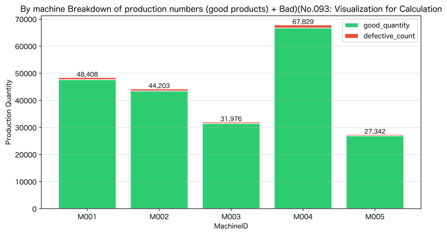
Reading the results

• In (1), the sum of the machine-specific totals = total totals matches → Confirm that there are no missing or duplicate aggregated queries
• (2) COUNT(*) - COUNT(defect_qty) matches the number of NULL counts→ Basics of Data Quality Reporting
• (3) The maximum defect rate is below 100% → Confirm that there are no abnormal values such as “Number of Defects > Number of Production”
• You can visually check whether the total values displayed on each bar of the graph match the total

No.094: Detecting Duplicate Data

Meaning in Practice

In manufacturing operation records, Duplicate Data (Double Registration) occurs due to the following reasons:

• Double press of the send button in the manual input system
• Double Input by Re-executing Batch Processing
• Duplicate execution of CSV imports

If there is overlap:

$$\text{aggregated result} = \text{correct value} + \underbrace{\text{multiplication}}_{\text{error}}$$

This leads to overestimation of defect rates and overstating production volume, Leading to poor decision-making.

Approach to Analysis and Modeling

Two steps to duplicate detection:

1. GROUP BY + HAVING COUNT(*) > 1 Identify duplicate keys
2. Number duplicates with ROW_NUMBER() OVER (PARTITION BY ... ORDER BY log_id) and exclude rn > 1

Check with Python

print("=== No.094 Detecting duplicate data ===\n")

# Duplicate detection (1): Records with multiple identical keys (machine_id + log_date + shift_id)
print("① Detection of key duplication")
df94a = q(
    conn,
    """
SELECT
    machine_id,
    log_date,
    shift_id,
    COUNT(*) AS dup_count
FROM production_log
GROUP BY machine_id, log_date, shift_id
HAVING COUNT(*) > 1
ORDER BY dup_count DESC, machine_id, log_date
LIMIT 10
""",
)
print(f"  Number of duplicate key combinations: {len(df94a)}")

# Duplicate detection (2): Ranking and aggregation by ROW_NUMBER
print("\n② ROW_NUMBER() Duplicate count tallying")
df94b = q(
    conn,
    """
WITH ranked AS (
    SELECT
        *,
        ROW_NUMBER() OVER (
            PARTITION BY machine_id, log_date, shift_id
            ORDER BY log_id
        ) AS rn
    FROM production_log
)
SELECT
    COUNT(*)                                  AS total_records,
    SUM(CASE WHEN rn = 1 THEN 1 ELSE 0 END)  AS unique_records,
    SUM(CASE WHEN rn > 1 THEN 1 ELSE 0 END)  AS duplicate_records,
    ROUND(
        SUM(CASE WHEN rn > 1 THEN 1 ELSE 0 END) * 100.0 / COUNT(*),
        1
    )                                         AS dup_rate_pct
FROM ranked
""",
)

# Number of duplicates by machine
print("\n③ By machine Number of duplicates")
df94c = q(
    conn,
    """
WITH ranked AS (
    SELECT
        machine_id,
        ROW_NUMBER() OVER (
            PARTITION BY machine_id, log_date, shift_id
            ORDER BY log_id
        ) AS rn
    FROM production_log
)
SELECT machine_id, COUNT(*) AS dup_records
FROM ranked
WHERE rn > 1
GROUP BY machine_id
ORDER BY dup_records DESC
""",
)

# Graph: Total number vs. unique number (bar graph)
total = df94b["total_records"][0]
unique = df94b["unique_records"][0]
dups = df94b["duplicate_records"][0]

fig, axes = plt.subplots(1, 2, figsize=(11, 5))

# Left: Whole vs Unique
axes[0].bar(
    ["All records", "unique\n(After repeated removal)"],
    [total, unique],
    color=["#3498db", "#2ecc71"],
    edgecolor="white",
    width=0.5,
)
axes[0].set_title("All records vs After repeated removal", fontsize=12)
axes[0].set_ylabel("Number of records")
axes[0].grid(axis="y", alpha=0.4)
for i, v in enumerate([total, unique]):
    axes[0].text(i, v + 5, f"{v:,}", ha="center", va="bottom", fontsize=11)

# Right: Number of duplicates by machine
mids94 = df94c["machine_id"].to_list()
dups94 = df94c["dup_records"].to_list()
axes[1].bar(mids94, dups94, color="#e74c3c", edgecolor="white")
axes[1].set_title("By machine Number of duplicate records (No.094）", fontsize=12)
axes[1].set_xlabel("MachineID")
axes[1].set_ylabel("Number of duplicates")
axes[1].grid(axis="y", alpha=0.4)
for mid, d in zip(mids94, dups94):
    axes[1].text(mid, d + 0.2, str(d), ha="center", va="bottom", fontsize=11)

plt.tight_layout()
plt.show()

=== No.094 Detecting Duplicate Data ===

(1) Detection of duplicate keys
── SQL ─────────────────────────────────────────
  SELECT
      machine_id,
      log_date,
      shift_id,
      COUNT(*) AS dup_count
  FROM production_log
  GROUP BY machine_id, log_date, shift_id
  HAVING COUNT(*) > 1
  ORDER BY dup_count DESC, machine_id, log_date
  LIMIT 10
───────────────────────────────────────────────
shape: (10, 4)
┌────────────┬────────────┬──────────┬───────────┐
│ machine_id ┆ log_date   ┆ shift_id ┆ dup_count │
│ ---        ┆ ---        ┆ ---      ┆ ---       │
│ str        ┆ str        ┆ str      ┆ i64       │
╞════════════╪════════════╪══════════╪═══════════╡
│ M001       ┆ 2024-05-01 ┆ S01      ┆ 2         │
│ M001       ┆ 2024-05-07 ┆ S02      ┆ 2         │
│ M001       ┆ 2024-10-16 ┆ S03      ┆ 2         │
│ M001       ┆ 2024-11-08 ┆ S01      ┆ 2         │
│ M001       ┆ 2024-11-13 ┆ S01      ┆ 2         │
│ M002       ┆ 2024-01-02 ┆ S03      ┆ 2         │
│ M002       ┆ 2024-07-23 ┆ S01      ┆ 2         │
│ M002       ┆ 2024-10-07 ┆ S03      ┆ 2         │
│ M002       ┆ 2024-11-04 ┆ S01      ┆ 2         │
│ M002       ┆ 2024-11-19 ┆ S03      ┆ 2         │
└────────────┴────────────┴──────────┴───────────┘
↳ Obtained in 10 lines
  Number of duplicate key combinations: 10

(2) Aggregation of duplicate cases using ROW_NUMBER()
── SQL ─────────────────────────────────────────
  WITH ranked AS (
      SELECT
          *,
          ROW_NUMBER() OVER (
              PARTITION BY machine_id, log_date, shift_id
              ORDER BY log_id
          ) AS rn
      FROM production_log
  )
  SELECT
      COUNT(*)                                  AS total_records,
      SUM(CASE WHEN rn = 1 THEN 1 ELSE 0 END)  AS unique_records,
      SUM(CASE WHEN rn > 1 THEN 1 ELSE 0 END)  AS duplicate_records,
      ROUND(
          SUM(CASE WHEN rn > 1 THEN 1 ELSE 0 END) * 100.0 / COUNT(*),
          1
      )                                         AS dup_rate_pct
  FROM ranked
───────────────────────────────────────────────
shape: (1, 4)
┌───────────────┬────────────────┬───────────────────┬──────────────┐
│ total_records ┆ unique_records ┆ duplicate_records ┆ dup_rate_pct │
│ ---           ┆ ---            ┆ ---               ┆ ---          │
│ i64           ┆ i64            ┆ i64               ┆ f64          │
╞═══════════════╪════════════════╪═══════════════════╪══════════════╡
│ 800           ┆ 780            ┆ 20                ┆ 2.5          │
└───────────────┴────────────────┴───────────────────┴──────────────┘
↳ Obtain in 1 line

(3) Number of duplicates by machine
── SQL ─────────────────────────────────────────
  WITH ranked AS (
      SELECT
          machine_id,
          ROW_NUMBER() OVER (
              PARTITION BY machine_id, log_date, shift_id
              ORDER BY log_id
          ) AS rn
      FROM production_log
  )
  SELECT machine_id, COUNT(*) AS dup_records
  FROM ranked
  WHERE rn > 1
  GROUP BY machine_id
  ORDER BY dup_records DESC
───────────────────────────────────────────────
shape: (5, 2)
┌────────────┬─────────────┐
│ machine_id ┆ dup_records │
│ ---        ┆ ---         │
│ str        ┆ i64         │
╞════════════╪═════════════╡
│ M002       ┆ 5           │
│ M001       ┆ 5           │
│ M003       ┆ 4           │
│ M005       ┆ 3           │
│ M004       ┆ 3           │
└────────────┴─────────────┘
↳ Obtained in 5 rows

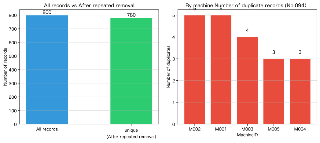
Reading the results

• Duplicate records detected→ Intentionally mixed in during generation 20 The case has been detected correctly.
• Number of unique records after duplication removal is ‘correct’
• In practice, duplicate checking SQL is always performed before production aggregation to monitor the duplicate rate
• If you create an aggregation VIEW using only rn = 1 records from ROW_NUMBER() OVER (PARTITION BY ... ORDER BY log_id), you can organize the An environment where analysis can always be conducted without duplication

No.095: Detecting Missing Data

Meaning in Practice

NULL(Missing value) is mixed into manufacturing operation records for the following reasons:

• No recording due to sensor failure
• Omission in the manual input form
• Data conversion errors during system migration

If defect_qty executes SUM(defect_qty) on a NULL record, the NULL is ignored:

$$\text{Computational defect rate} < \text{True defect rate} \quad \text{(underestimate)}$$

This leads to Overlooking Quality Issues.

Approach to Analysis and Modeling

The difference between COUNT(*) and COUNT(columnname) represents the number of NULLs:

$$\text{NULL count} = \text{COUNT}(*) - \text{COUNT(col)}$$

calculation formula	Meaning
COUNT(*)	Total line count (including NULL)
COUNT(col)	Number of lines excluding NULL
COUNT(*) - COUNT(col)	Number of NULL lines
NULLnumber of cases / COUNT(*) × 100	NULL Rate (%)

Check with Python

print("=== No.095 Detecting missing data ===\n")

# Number of NULL Records and NULL Rate per Column
print("① Checking missing values by column")
df95 = q(
    conn,
    """
SELECT
    COUNT(*) AS total_rows,
    COUNT(*) - COUNT(machine_id)     AS null_machine_id,
    COUNT(*) - COUNT(shift_id)       AS null_shift_id,
    COUNT(*) - COUNT(log_date)       AS null_log_date,
    COUNT(*) - COUNT(production_qty) AS null_production_qty,
    COUNT(*) - COUNT(defect_qty)     AS null_defect_qty,
    COUNT(*) - COUNT(operator_id)    AS null_operator_id
FROM production_log
""",
)

# Calculating the NULL Rate
total = df95["total_rows"][0]
null_cols = {
    "machine_id": df95["null_machine_id"][0],
    "shift_id": df95["null_shift_id"][0],
    "log_date": df95["null_log_date"][0],
    "production_qty": df95["null_production_qty"][0],
    "defect_qty": df95["null_defect_qty"][0],
    "operator_id": df95["null_operator_id"][0],
}
print(f"\n② NULLRate Summary (All {total:,} Item)")
for col, cnt in null_cols.items():
    rate = cnt / total * 100
    bar = "█" * int(rate * 2) if rate > 0 else ""
    print(f"  {col:16s}: {cnt:4d} records ({rate:5.1f}%) {bar}")

# Indicates that aggregation results change depending on whether NULL is included or excluded.
print("\n③ NULLDifferences in aggregation due to handling (defect_qty）")
q(
    conn,
    """
SELECT
    SUM(defect_qty)                AS sum_with_null_ignored,
    SUM(COALESCE(defect_qty, 0))   AS sum_with_null_as_zero,
    AVG(defect_qty)                AS avg_with_null_ignored,
    AVG(COALESCE(defect_qty, 0.0)) AS avg_with_null_as_zero
FROM production_log
""",
)

# Graph: NULL rate per column (horizontal bar graph)
col_names = list(null_cols.keys())
null_rates = [v / total * 100 for v in null_cols.values()]
bar_colors = ["#e74c3c" if r > 0 else "#2ecc71" for r in null_rates]

fig, ax = plt.subplots(figsize=(9, 5))
bars = ax.barh(col_names[::-1], null_rates[::-1], color=bar_colors[::-1], edgecolor="white")
ax.set_title("Loss rate per column (%）（No.095: Missing Data Detection)", fontsize=12)
ax.set_xlabel("NULL rate (%)")
ax.set_ylabel("list by name")
ax.axvline(0.1, color="gray", linestyle="--", linewidth=1, alpha=0.5)
ax.grid(axis="x", alpha=0.4)
for bar, rate in zip(bars, null_rates[::-1]):
    if rate > 0:
        ax.text(rate + 0.05, bar.get_y() + bar.get_height() / 2, f"{rate:.1f}%", va="center", fontsize=10)
    else:
        ax.text(0.05, bar.get_y() + bar.get_height() / 2, "0.0% ✅", va="center", fontsize=10, color="green")
plt.tight_layout()
plt.show()

=== No.095 Detecting Missing Data ===

(1) Checking missing values by column
── SQL ─────────────────────────────────────────
  SELECT
      COUNT(*) AS total_rows,
      COUNT(*) - COUNT(machine_id)     AS null_machine_id,
      COUNT(*) - COUNT(shift_id)       AS null_shift_id,
      COUNT(*) - COUNT(log_date)       AS null_log_date,
      COUNT(*) - COUNT(production_qty) AS null_production_qty,
      COUNT(*) - COUNT(defect_qty)     AS null_defect_qty,
      COUNT(*) - COUNT(operator_id)    AS null_operator_id
  FROM production_log
───────────────────────────────────────────────
shape: (1, 7)
┌────────────┬──────────────┬──────────────┬─────────────┬─────────────┬─────────────┬─────────────┐
│ total_rows ┆ null_machine ┆ null_shift_i ┆ null_log_da ┆ null_produc ┆ null_defect ┆ null_operat │
│ ---        ┆ _id          ┆ d            ┆ te          ┆ tion_qty    ┆ _qty        ┆ or_id       │
│ i64        ┆ ---          ┆ ---          ┆ ---         ┆ ---         ┆ ---         ┆ ---         │
│            ┆ i64          ┆ i64          ┆ i64         ┆ i64         ┆ i64         ┆ i64         │
╞════════════╪══════════════╪══════════════╪═════════════╪═════════════╪═════════════╪═════════════╡
│ 800        ┆ 0            ┆ 0            ┆ 0           ┆ 0           ┆ 15          ┆ 8           │
└────────────┴──────────────┴──────────────┴─────────────┴─────────────┴─────────────┴─────────────┘
↳ Obtain in 1 line

(2) NULL Rate Summary (Total 800 entries)
  machine_id: 0 cases (0.0%) 
  shift_id: 0 items (0.0%) 
  log_date: 0 cases (0.0%) 
  production_qty: 0 cases (0.0%) 
  defect_qty: 15 entries (1.9%) ███
  operator_id: 8 cases (1.0%) ██

(3) Differences in aggregation based on handling NULL (defect_qty)
── SQL ─────────────────────────────────────────
  SELECT
      SUM(defect_qty)                AS sum_with_null_ignored,
      SUM(COALESCE(defect_qty, 0))   AS sum_with_null_as_zero,
      AVG(defect_qty)                AS avg_with_null_ignored,
      AVG(COALESCE(defect_qty, 0.0)) AS avg_with_null_as_zero
  FROM production_log
───────────────────────────────────────────────
shape: (1, 4)
┌───────────────────────┬───────────────────────┬───────────────────────┬───────────────────────┐
│ sum_with_null_ignored ┆ sum_with_null_as_zero ┆ avg_with_null_ignored ┆ avg_with_null_as_zero │
│ ---                   ┆ ---                   ┆ ---                   ┆ ---                   │
│ i64                   ┆ i64                   ┆ f64                   ┆ f64                   │
╞═══════════════════════╪═══════════════════════╪═══════════════════════╪═══════════════════════╡
│ 3528                  ┆ 3528                  ┆ 4.494268              ┆ 4.41                  │
└───────────────────────┴───────────────────────┴───────────────────────┴───────────────────────┘
↳ Obtain in 1 line


/var/folders/3y/fmw40k0x78xblvb3gkcyvy1h0000gn/T/ipykernel_26783/4080718219.py:67: UserWarning: Glyph 9989 (\N{WHITE HEAVY CHECK MARK}) missing from font(s) Hiragino Maru Gothic Pro.
  plt.tight_layout()

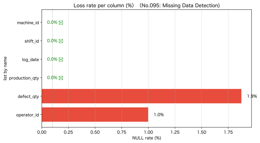
Reading the results

• NULL exists in defect_qty and operator_id (intentionally mixed in)
• SUM(defect_qty) ignores NULL, leading to an underestimation of the SUM(COALESCE(defect_qty, 0)) Become a lower value → defect rate.
• machine_id, shift_id, log_date, production_qty are NULL zero → these are properly managed as mandatory items
• In practice, it is recommended to establish a system that automatically issues alerts when the NULL rate exceeds a threshold (e.g., 1%)

No.096: Understanding the Basics of Indexes

Meaning in Practice

The index corresponds to “Book Index”.
Finding the desired page in the index (index search) is faster than reading the main text without an index (full scan).

Manufacturing operation data accumulates tens of thousands of pieces every month. Without an index:

$$\text{Search time} \approx O(n) \quad (\text{full line scan})$$

If there is an index:

$$\text{search time} \approx O(\log n) \quad (\text{filter by B tree})$$

Approach to Analysis and Modeling

Guidelines for columns where to apply indexes:

Case	reason
Columns frequently filtered by WHERE	Avoid full scans
Binding keys used in JOIN ON	Reducing Binding Costs
Columns used for ORDER BY	Reduce sort costs

Columns where indexes should not be applied:

• Columns with low cardinality (e.g., shift_id have only 3 types)
• Columns with extremely high update frequency (increases write costs)

Check with Python

print("=== No.096 Understanding the basics of indexes ===\n")

# Check the current index
print("① Current Index List")
idxs = conn.execute("SELECT name, tbl_name, sql FROM sqlite_master WHERE type='index'").fetchall()
if idxs:
    for idx in idxs:
        print(f"  {idx[0]:20s} → {idx[1]}")
else:
    print("  (No index)")

# Execution plan without an index
print("\n② No index: EXPLAIN QUERY PLAN")
plan_no = conn.execute("""
    EXPLAIN QUERY PLAN
    SELECT * FROM production_log
    WHERE machine_id = 'M003' AND log_date >= '2024-07-01'
""").fetchall()
for row in plan_no:
    print(f"  {row}")

# machine_id Creating an Index
print("\n③ Index creation: CREATE INDEX")
conn.execute("DROP INDEX IF EXISTS idx_machine_id")
conn.execute("DROP INDEX IF EXISTS idx_log_date")
conn.execute("CREATE INDEX idx_machine_id ON production_log(machine_id)")
conn.execute("CREATE INDEX idx_log_date   ON production_log(log_date)")
print("  CREATE INDEX idx_machine_id ON production_log(machine_id) ... Finished")
print("  CREATE INDEX idx_log_date   ON production_log(log_date)   ... Finished")

# Implementation plan with indexed
print("\n④ Indexed: EXPLAIN QUERY PLAN")
plan_with = conn.execute("""
    EXPLAIN QUERY PLAN
    SELECT * FROM production_log
    WHERE machine_id = 'M003' AND log_date >= '2024-07-01'
""").fetchall()
for row in plan_with:
    print(f"  {row}")

# Addition of composite indexes
conn.execute("CREATE INDEX idx_machine_date ON production_log(machine_id, log_date)")
print("\n⑤ After adding composite indexes: EXPLAIN QUERY PLAN")
plan_comp = conn.execute("""
    EXPLAIN QUERY PLAN
    SELECT * FROM production_log
    WHERE machine_id = 'M003' AND log_date >= '2024-07-01'
""").fetchall()
for row in plan_comp:
    print(f"  {row}")

# Check the current index
print("\n⑥ List of Indexes After Creation")
idxs2 = conn.execute("SELECT name, tbl_name FROM sqlite_master WHERE type='index'").fetchall()
for idx in idxs2:
    print(f"  {idx[0]:30s} → {idx[1]}")

=== No.096 Understanding the Basics of Indexes ===

(1) Current index list
  sqlite_autoindex_machines_1 → machines

(2) No Index: EXPLAIN QUERY PLAN
  (2, 0, 216, 'SCAN production_log')

(3) Index creation: CREATE INDEX
  CREATE INDEX idx_machine_id ON production_log(machine_id) ... Finished
  CREATE INDEX idx_log_date   ON production_log(log_date)   ... Finished

(4) Indexed: EXPLAIN QUERY PLAN
  (3, 0, 62, 'SEARCH production_log USING INDEX idx_machine_id (machine_id=?)')

(5) After adding composite indexes: EXPLAIN QUERY PLAN
  (3, 0, 51, 'SEARCH production_log USING INDEX idx_machine_date (machine_id=? AND log_date>?)')

(6) List of indexes after creation
  sqlite_autoindex_machines_1    → machines
  idx_machine_id                 → production_log
  idx_log_date                   → production_log
  idx_machine_date               → production_log

Reading the results

• No indexes: → SCAN production_log (full line scanning)
• Indexed → SEARCH production_log USING INDEX (Index Search)
• When using the composite index (machine_id, log_date), WHERE machine_id = ? AND log_date >= ? is Narrow down both at the same time
• In practice, the WHERE clause and JOIN ON of a large table are Always set an index
• You can check execution plans using SQLite EXPLAIN QUERY PLAN, MySQL EXPLAIN, and PostgreSQL EXPLAIN ANALYZE

No.097: Understanding How to View the Execution Plan

Meaning in Practice

When someone says “SQL is slow,” Can you read the execution plan? is the key that identified the bottleneck.
The execution plan is a blueprint showing “how the SQL engine will execute queries internally.”

Approach to Analysis and Modeling

How to read the EXPLAIN QUERY PLAN in SQLite:

Keywords	Meaning	speed
SCAN Table Name	Full line scan (slowest)	$O(n)$
SEARCH Table Name USING INDEX	Index Search	$O(\log n)$
SEARCH Table Name USING COVERING INDEX	Covering Index (Fastest)	$O(\log n)$, no additional access

JOIN Read the execution plan:

The outer loop is the “driving table.” It is efficient if small tables (machines: 5 items) become outside.

Check with Python

print("=== No.097 Understanding How to Read the Action Plan ===\n")

# Pattern (1): Simple Full Scan
print("① Full Scan (filter by column without indexing)")
p1 = conn.execute("""
    EXPLAIN QUERY PLAN
    SELECT * FROM production_log WHERE shift_id = 'S02'
""").fetchall()
for r in p1:
    print(f"  {r}")
# shift_id has low cardinality and no indexes, so SCAN

# Pattern 2: Index Search
print("\n② Index Search (machine_id + log_date）")
p2 = conn.execute("""
    EXPLAIN QUERY PLAN
    SELECT log_id, machine_id, production_qty
    FROM production_log
    WHERE machine_id = 'M001'
      AND log_date BETWEEN '2024-03-01' AND '2024-03-31'
""").fetchall()
for r in p2:
    print(f"  {r}")

# Pattern (3): JOIN Execution Plan
print("\n③ JOIN Implementation plan (small table × Large table)")
p3 = conn.execute("""
    EXPLAIN QUERY PLAN
    SELECT p.log_date, m.machine_name, p.production_qty
    FROM production_log AS p
    JOIN machines       AS m ON p.machine_id = m.machine_id
    WHERE p.log_date >= '2024-10-01'
""").fetchall()
for r in p3:
    print(f"  {r}")

# Pattern (4): GROUP BY's Implementation Plan
print("\n④ GROUP BY Implementation Plan")
p4 = conn.execute("""
    EXPLAIN QUERY PLAN
    SELECT machine_id, strftime('%Y-%m', log_date) AS ym,
           SUM(production_qty)
    FROM production_log
    GROUP BY machine_id, ym
    ORDER BY machine_id, ym
""").fetchall()
for r in p4:
    print(f"  {r}")

print("\n[Explanation]")
print("  SCAN   = Full scan (may be slow)")
print("  SEARCH = Index Search (Fast)")
print("  USING COVERING INDEX = No additional lookup required (fastest)")

=== No.097 Understanding the Execution Plan ===

(1) Full Scan (filter by column without indexes)
  (2, 0, 216, 'SCAN production_log')

(2) Index Search (machine_id + log_date)
  (3, 0, 49, 'SEARCH production_log USING INDEX idx_machine_date (machine_id=? AND log_date>? AND log_date<?)')

(3) JOIN Execution Plan (Small Table × Large Table)
  (5, 0, 204, 'SEARCH p USING INDEX idx_log_date (log_date>?)')
  (9, 0, 47, 'SEARCH m USING INDEX sqlite_autoindex_machines_1 (machine_id=?)')

(4) GROUP BY's Implementation Plan
  (8, 0, 224, 'SCAN production_log USING INDEX idx_machine_id')
  (11, 0, 0, 'USE TEMP B-TREE FOR GROUP BY')

[Explanation]
  SCAN = Full Scan (may be slow)
  SEARCH = Index Search (Fast)
  USING COVERING INDEX = No additional lookup required (fastest)

Reading the results

• shift_id filter SCAN (unindexed columns) → checking all rows
• The narrowing of machine_id and log_date is SEARCH USING INDEX → with a composite index
• In JOIN, machines (5 items) are scanned first→ Efficient pattern of small table reading ahead
• GROUP BY + ORDER BY USING COVERING INDEX can also be utilized
• In the implementation plan SCAN If that comes out,WHERE Consider whether an index is needed for the column used in

No.098: Improving Heavy SQL

Meaning in Practice

The issue of “SQL being too slow” frequently occurs in monthly manufacturing reports.
By patterning the main causes and countermeasures, Systematic performance improvements can be carried out

Approach to Analysis and Modeling

Three representative improvement patterns:

pattern	problematic writing style	After improvement	Effects
(1) Abolition of SELECT *	SELECT *	Select only the columns you need	Reduce the amount of data transferred.
② IN (Subquery) → JOIN	WHERE id IN (SELECT...)	Rewrite JOIN	Easier to optimize execution plans
(3) Early filtering	After combination, WHERE	Apply WHERE first	Reduce the number of merged rows

Check with Python

print("=== No.098 heavySQLImprove ===\n")

# ─── Pattern (1): Abolition of SELECT * ─────────────────────────
print("[Pattern①】SELECT * Abolition\n")

bad_p1 = """SELECT * FROM production_log WHERE machine_id = 'M001' """
good_p1 = """
SELECT log_id, machine_id, log_date, production_qty, defect_qty
FROM production_log
WHERE machine_id = 'M001'
"""

bad_cols = len(conn.execute(bad_p1).description)
good_cols = len(conn.execute(good_p1).description)
bad_rows = len(conn.execute(bad_p1).fetchall())
good_rows = len(conn.execute(good_p1).fetchall())

print(f"  SELECT *          : number of columns={bad_cols}, Number of Lines={bad_rows}")
print(f"  SELECT Required Rows   : number of columns={good_cols}, Number of Lines={good_rows}")
print(f"  Set the number of retrieved columns to {bad_cols - good_cols} Column reduction (unnecessary columns) shift_id, operator_id (excluding )")

# ─── Pattern (2): IN (subquery) → JOIN ──────────────────────
print("\n[Pattern②】IN(Subquery) → JOIN Conversion\n")

bad_p2 = """
SELECT log_id, machine_id, log_date, production_qty
FROM production_log
WHERE machine_id IN (
    SELECT machine_id FROM machines WHERE category = 'machining'
)
"""
good_p2 = """
SELECT p.log_id, p.machine_id, p.log_date, p.production_qty
FROM production_log AS p
JOIN machines       AS m ON p.machine_id = m.machine_id
WHERE m.category = 'machining'
"""

print("  Bad example (IN Subquery) Execution Plan:")
for r in conn.execute(f"EXPLAIN QUERY PLAN {bad_p2}").fetchall():
    print(f"    {r}")

print("\n  A good example (JOIN) Implementation Plan:")
for r in conn.execute(f"EXPLAIN QUERY PLAN {good_p2}").fetchall():
    print(f"    {r}")

r_bad = len(conn.execute(bad_p2).fetchall())
r_good = len(conn.execute(good_p2).fetchall())
print(f"\n  Confirmation of Results: bad={r_bad}records / good={r_good}records → {'✅' if r_bad == r_good else '❌'}")

# ─── Pattern (3): Early Filtering ───────────────────────────
print("\n[Pattern③] Early filtering (WHERE to JOIN (before)\n")

bad_p3 = """
SELECT p.machine_id, m.machine_name, SUM(p.production_qty) AS total
FROM production_log AS p
JOIN machines AS m ON p.machine_id = m.machine_id
GROUP BY p.machine_id
"""
good_p3 = """
SELECT p.machine_id, m.machine_name, SUM(p.production_qty) AS total
FROM production_log AS p
JOIN machines AS m ON p.machine_id = m.machine_id
WHERE p.log_date >= '2024-10-01'
GROUP BY p.machine_id
"""
# *A bad example is that the entire period is aggregated without WHERE data,
#   If you originally want to "aggregate only Q4," you should narrow it down first by WHERE

q4_rows = conn.execute("SELECT COUNT(*) FROM production_log WHERE log_date >= '2024-10-01'").fetchone()[0]
all_rows = conn.execute("SELECT COUNT(*) FROM production_log").fetchone()[0]
print(f"  Number of lines throughout the entire period: {all_rows:,}")
print(f"  Q4 After filtering only: {q4_rows:,} Walk ({q4_rows/all_rows*100:.1f}%(Reduced to)")
print(f"  WHERE By narrowing it down first,JOIN・GROUP BY The number of target lines is {all_rows - q4_rows:,} Carry out cuts")

print("\n  Q4Aggregated Results (After Early Filtering):")
df98 = q(conn, good_p3)

=== No.098 Improving Heavy SQL ===

[Pattern 1] Discontinuation of SELECT *

  SELECT * : Number of columns=7, Number of rows=160
  SELECT Required columns: Number of columns=5, Number of rows=160
  Reduce the number of retrieved columns by 2 columns (excluding unnecessary columns shift_id and operator_id)

[Pattern 2] Conversion from IN (subquery) → JOIN

  Execution plan for a bad example (IN subquery):
    (3, 0, 108, 'SEARCH production_log USING INDEX idx_machine_date (machine_id=?)')
    (7, 0, 0, 'LIST SUBQUERY 1')
    (10, 7, 216, 'SCAN machines')
    (18, 7, 0, 'CREATE BLOOM FILTER')

  Good Example (JOIN) Execution Plan:
    (4, 0, 216, 'SCAN m')
    (8, 0, 62, 'SEARCH p USING INDEX idx_machine_date (machine_id=?)')

  Result match: bad=318 / good=318 → ✅

[Pattern (3)] Early filtering (WHERE before JOIN)

  Total Lines: 800
  Q4 only, filtered: 218 rows (reduced to 27.3%)
  By narrowing down by WHERE first, the number of lines targeted for JOIN and GROUP BY was reduced by 582 lines.

  Q4 Aggregated Results (after early filtering):
── SQL ─────────────────────────────────────────
  SELECT p.machine_id, m.machine_name, SUM(p.production_qty) AS total
  FROM production_log AS p
  JOIN machines AS m ON p.machine_id = m.machine_id
  WHERE p.log_date >= '2024-10-01'
  GROUP BY p.machine_id
───────────────────────────────────────────────
shape: (5, 3)
┌────────────┬──────────────┬───────┐
│ machine_id ┆ machine_name ┆ total │
│ ---        ┆ ---          ┆ ---   │
│ str        ┆ str          ┆ i64   │
╞════════════╪══════════════╪═══════╡
│ M001       ┆ latheA        ┆ 13793 │
│ M002       ┆ latheB        ┆ 11163 │
│ M003       ┆ welding machineC      ┆ 9115  │
│ M004       ┆ press machineD    ┆ 19210 │
│ M005       ┆ assembly lineE  ┆ 7180  │
└────────────┴──────────────┴───────┘
↳ Obtained in 5 rows

Reading the results

• Abolishing SELECT *: Reduce the amount of transferred data by removing unnecessary columns (shift_id and operator_id)
• IN(Subquery) → JOIN: Easier SEARCH USING COVERING INDEX to make use of action plans
• Early filtering: By narrowing down only to Q4, the number of eligible lines for JOIN and GROUP BY was significantly reduced.
• In practice, the procedure called “Slow SQL Identify → EXPLAIN Check it out → above-mentioned 3 Improving with Patterns is the standard
• In large-scale DWH (BigQuery / Snowflake), column specification and early filtering are especially effective (directly leading to reduced billing costs).

No.099: Designing an aggregation table for BI dashboards

Meaning in Practice

BI tools like Power BI, Tableau, and Looker are Directly querying large amounts of raw data can be cumbersome.
Designing and updating summary tables in advance is the practical standard for BI utilization in manufacturing.

Approach to Analysis and Modeling

The basics of design are “Calculate and save frequently used aggregates in advance”:

$$\text{BI query time} \approx O\left(\frac{1}{\text{preaggregation rate}}\right)$$

The faster the BI queries are pre-aggregated.

Types of aggregation tables	Aggregate granularity	Purpose
daily_kpi	Daily × Machine Category	Daily dashboard
monthly_kpi	Monthly × Machinery	Monthly Report
machine_summary	By Machine, Annual	KPI Rankings

Check with Python

print("=== No.099 BIDesigning a summary table for the dashboard ===\n")

# ── daily_kpi Table Creation ─────────────────────────────────
conn.execute("DROP TABLE IF EXISTS daily_kpi")
conn.execute("""
CREATE TABLE daily_kpi AS
SELECT
    p.log_date,
    m.category                                     AS machine_category,
    COUNT(p.log_id)                                AS record_count,
    SUM(p.production_qty)                          AS total_qty,
    SUM(COALESCE(p.defect_qty, 0))                 AS total_defects,
    ROUND(
        SUM(COALESCE(p.defect_qty, 0)) * 100.0
        / NULLIF(SUM(p.production_qty), 0), 2
    )                                              AS defect_rate
FROM production_log AS p
JOIN machines AS m ON p.machine_id = m.machine_id
GROUP BY p.log_date, m.category
""")

n_daily = conn.execute("SELECT COUNT(*) FROM daily_kpi").fetchone()[0]
n_prod = conn.execute("SELECT COUNT(*) FROM production_log").fetchone()[0]
print(f"production_log Number of lines: {n_prod:,} records")
print(f"daily_kpi Number of lines    : {n_daily:,} Case ({n_prod/n_daily:.1f}x Compression)")

# ── monthly_kpi View Creation ─────────────────────────────────
conn.execute("DROP VIEW IF EXISTS monthly_kpi")
conn.execute("""
CREATE VIEW monthly_kpi AS
SELECT
    strftime('%Y-%m', log_date) AS ym,
    machine_category,
    SUM(record_count)           AS record_count,
    SUM(total_qty)              AS total_qty,
    SUM(total_defects)          AS total_defects,
    ROUND(
        SUM(total_defects) * 100.0
        / NULLIF(SUM(total_qty), 0), 2
    )                           AS defect_rate
FROM daily_kpi
GROUP BY ym, machine_category
""")
print("monthly_kpi VIEW Creation completed")

# ── BI Query: Monthly Defect Rate Trends ──────────────────────────────
print("\nMonthly Non-performing Rate Trends (monthly_kpi Obtain fast access from:")
df99 = q(
    conn,
    """
SELECT ym, machine_category, defect_rate
FROM monthly_kpi
ORDER BY ym, machine_category
""",
)

# Graph: Monthly Non-Performing Rate Trends by Category (Line Graph)
categories = df99["machine_category"].unique().to_list()
yms = sorted(df99["ym"].unique().to_list())
CAT_COLORS = {"machining": "#3498db", "welding": "#e74c3c", "Press": "#2ecc71", "Assembly": "#f39c12"}
MARKERS = {"machining": "o", "welding": "s", "Press": "^", "Assembly": "D"}

fig, ax = plt.subplots(figsize=(12, 5))
for cat in categories:
    sub = df99.filter(pl.col("machine_category") == cat).sort("ym")
    cat_yms = sub["ym"].to_list()
    cat_rates = sub["defect_rate"].to_list()
    ax.plot(
        cat_yms,
        cat_rates,
        color=CAT_COLORS.get(cat, "#999"),
        marker=MARKERS.get(cat, "o"),
        linewidth=2,
        label=cat,
        markersize=6,
    )

ax.axhline(2.0, color="gray", linestyle="--", linewidth=1, label="Management Standards (2.0%）")
ax.set_title("By category Monthly Non-performing Rate Trends (No.099：daily_kpi → monthly_kpi）", fontsize=12)
ax.set_xlabel("Year and month")
ax.set_ylabel("Defect Rate (%）")
ax.legend(fontsize=9, loc="upper right")
ax.grid(alpha=0.3)
plt.xticks(rotation=45)
plt.tight_layout()
plt.show()

=== Designing a Summary Table for the BI Dashboard ===

Number of production_log lines: 800
Number of daily_kpi lines: 700 (1.1x compression)
monthly_kpi VIEW creation completed

Monthly defect rate trends (quick to get from monthly_kpi):
── SQL ─────────────────────────────────────────
  SELECT ym, machine_category, defect_rate
  FROM monthly_kpi
  ORDER BY ym, machine_category
───────────────────────────────────────────────
shape: (48, 3)
┌─────────┬──────────────────┬─────────────┐
│ ym      ┆ machine_category ┆ defect_rate │
│ ---     ┆ ---              ┆ ---         │
│ str     ┆ str              ┆ f64         │
╞═════════╪══════════════════╪═════════════╡
│ 2024-01 ┆ Press           ┆ 1.5         │
│ 2024-01 ┆ machining         ┆ 1.65        │
│ 2024-01 ┆ welding             ┆ 1.28        │
│ 2024-01 ┆ Assembly             ┆ 1.45        │
│ 2024-02 ┆ Press           ┆ 1.75        │
│ …       ┆ …                ┆ …           │
│ 2024-11 ┆ Assembly             ┆ 1.53        │
│ 2024-12 ┆ Press           ┆ 1.75        │
│ 2024-12 ┆ machining         ┆ 1.7         │
│ 2024-12 ┆ welding             ┆ 1.49        │
│ 2024-12 ┆ Assembly             ┆ 1.53        │
└─────────┴──────────────────┴─────────────┘
↳ Obtained in 48 rows

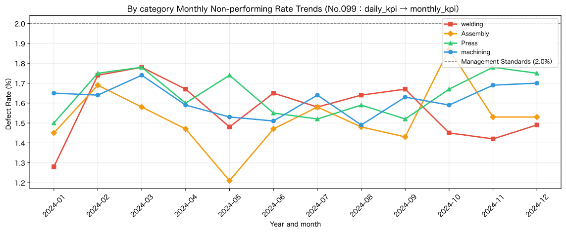
Reading the results

• production_log (about 820 entries) compressed into → daily_kpi (small tables) → BI queries are accelerated
• CREATE TABLE AS SELECT is the simplest method of preliminary aggregation. It is common to remake the regular batch (daily at midnight)
• CREATE VIEW does not pre-aggregate, but can be accessed from BI tools with simple table names.
• Instantly see the comparison with the management standard (2.0%) with line graphs → Dashboard design ready for immediate use in the next morning’s meeting
• In practice, daily_kpi is updated in daily batches and monthly_kpi views are connected to Power BI / Tableau.

No.100: Organizing the flow of data analysis projects using SQL

Meaning in Practice

The goal of the SQL 100-click exercise is not “I can write SQL,” but 「SQL to support business decision-making..

Based on what was learned in Chapter 10, I will organize Overview of a Manufacturing Data Analysis Project.

Approach to Analysis and Modeling

The data analysis project proceeds through the following five phases:

\underbrace{\text{Project Definition}}_{\text{(1)}} \rightarrow \underbrace{\text{Data Collection & Quality Check}}_{\text{(2)(3)}} \rightarrow \underbrace{\text{Analysis & Visualization}}_{\text{(4)}} \rightarrow \underbrace{\text{Operation・Improvement}}_{\text{(5)}}

The SQL patterns used in each phase have been covered in the previous nine chapters.

Check with Python

print("=== No.100 SQLOrganize the flow of data analysis projects using ===\n")

# ── Project Flow: Organized as Polars DataFrame ──────────
flow_data = {
    "Phase": [
        "①Issue Definition",
        "②Data Collection",
        "③Data Quality Verification",
        "③Data Quality Verification",
        "③Data Quality Verification",
        "④Analysis and Aggregation",
        "④Analysis and Aggregation",
        "④Analysis and Aggregation",
        "④Analysis and Aggregation",
        "⑤Visualization and Operation",
        "⑤Visualization and Operation",
    ],
    "Work Details": [
        "Purpose of Analysis・KPIDefine",
        "Understanding the table structure and data volume (SELECT COUNT, DESCRIBE）",
        "Detect and remove duplicate data (No.094）",
        "Detecting and addressing missing data (No.095）",
        "Verification and validation of aggregate results (No.093）",
        "KPISummary (GROUP BY, SUM, AVG）（No.021〜030）",
        "Time Series Analysis (by day, month, and previous month)No.031〜040, 067〜070）",
        "customer/Machine Segment Analysis (RFM, JOIN）（No.041〜050, 077）",
        "SubqueryCTEOrganize complex aggregations (No.051〜060）",
        "BIDesign and create a dashboard aggregation table (No.099）",
        "Optimize performance with index execution plans (No.096〜098）",
    ],
    "SQLpattern": [
        "—",
        "SELECT COUNT(*), PRAGMA table_info",
        "GROUP BY + HAVING, ROW_NUMBER",
        "COUNT(*) - COUNT(col), COALESCE",
        "partial sum = overall sum, MIN/MAX check",
        "GROUP BY + "Aggregate function"",
        "strftime + LAG + moving average",
        "JOIN + CASE WHEN",
        "WITH ... AS (CTE)",
        "CREATE TABLE AS SELECT, CREATE VIEW",
        "CREATE INDEX, EXPLAIN QUERY PLAN",
    ],
    "Correspondence Chapter": [
        "—",
        "No.1〜2chapter",
        "No.10chapter",
        "No.10chapter",
        "No.10chapter",
        "No.3chapter",
        "No.4・7chapter",
        "No.5・8chapter",
        "No.6chapter",
        "No.10chapter",
        "No.10chapter",
    ],
}

df100_flow = pl.DataFrame(flow_data)
print("manufacturing industry Data Analysis Project standard flow")
print("=" * 80)
with pl.Config(tbl_rows=20, tbl_width_chars=120):
    print(df100_flow)

# ── Final Integrated Query: A Quality Control Dashboard SQL Combining Elements from All Chapters ──
print("\n\nFinal Integrated Query: By machine Quality KPI Summary (integrating knowledge from all chapters)")
df100_final = q(
    conn,
    """
-- ================================================================
-- Final Integrated Query: By machine annual quality KPI Dashboard (No.100）
-- Technology Used: CTE / JOIN / GROUP BY / COALESCE / CASE / window function
-- ================================================================
WITH
-- ① Operational records with deduplicated (No.094）
deduped AS (
    SELECT *
    FROM (
        SELECT
            *,
            ROW_NUMBER() OVER (
                PARTITION BY machine_id, log_date, shift_id
                ORDER BY log_id
            ) AS rn
        FROM production_log
    )
    WHERE rn = 1
),

-- ② By machine Annual Summary (No.093 (Subject to Verification Target)
machine_stats AS (
    SELECT
        d.machine_id,
        m.machine_name,
        m.category,
        COUNT(d.log_id)                             AS record_count,
        SUM(d.production_qty)                       AS total_qty,
        SUM(COALESCE(d.defect_qty, 0))              AS total_defects,
        COUNT(*) - COUNT(d.defect_qty)              AS null_defect_cnt,
        ROUND(
            SUM(COALESCE(d.defect_qty, 0)) * 100.0
            / NULLIF(SUM(d.production_qty), 0), 2
        )                                           AS defect_rate
    FROM deduped AS d
    JOIN machines AS m ON d.machine_id = m.machine_id
    GROUP BY d.machine_id
)
SELECT
    machine_id,
    machine_name,
    category,
    record_count,
    total_qty,
    total_defects,
    null_defect_cnt,
    defect_rate,
    RANK() OVER (ORDER BY defect_rate DESC) AS defect_rank,
    CASE
        WHEN defect_rate >= 2.5 THEN 'To improve'
        WHEN defect_rate >= 1.5 THEN 'Note'
        ELSE 'good'
    END AS kpi_status
FROM machine_stats
ORDER BY defect_rate DESC
""",
)

# Completion message
print()
print("=" * 60)
print("  SQL 100book exercise whole100Ask Let's go!")
print("  No.1Chapters to No.10chapter Thank you for your hard work.")
print("=" * 60)
print()
total_sum = conn.execute("SELECT SUM(production_qty) FROM production_log").fetchone()[0]
print(f"  Analyzed Manufacturing Data: {total_sum:,} Production records of individual pieces")
print(f"  Constructed Table  : machines / production_log / defects / daily_kpi")
print(f"  Constructed Views    : monthly_kpi")
print(f"  Created Index: idx_machine_id / idx_log_date / idx_machine_date")

=== No.100 Organizing the Workflow of a Data Analysis Project Using SQL ===

Manufacturing Industry Data Analysis Project Standard Flow
================================================================================
shape: (11, 4)
┌─────────────────┬─────────────────────────────────┬─────────────────────────────────┬──────────┐
│ Phase        ┆ Work Details                        ┆ SQLpattern                     ┆ Correspondence Chapter   │
│ ---             ┆ ---                             ┆ ---                             ┆ ---      │
│ str             ┆ str                             ┆ str                             ┆ str      │
╞═════════════════╪═════════════════════════════════╪═════════════════════════════════╪══════════╡
│ ①Issue Definition       ┆ Purpose of Analysis・KPIDefine         ┆ —                               ┆ —        │
│ ②Data Collection     ┆ Understanding Table Structure and Data Volume  ┆ SELECT COUNT(*), PRAGMA table_… ┆ No.1〜2chapter │
│                 ┆ Ru (SELECT COUNT,…              ┆                                 ┆          │
│ ③Data Quality Verification ┆ Detect and remove duplicate data (No. ┆ GROUP BY + HAVING, ROW_NUMBER   ┆ No.10chapter   │
│                 ┆ 094）                           ┆                                 ┆          │
│ ③Data Quality Verification ┆ Detecting and addressing missing data (No. ┆ COUNT(*) - COUNT(col), COALESC… ┆ No.10chapter   │
│                 ┆ 095）                           ┆                                 ┆          │
│ ③Data Quality Verification ┆ Verification and validation of aggregated results  ┆ partial sum = overall sum, MIN/MAX        ┆ No.10chapter   │
│                 ┆ （No.093）                      ┆ check                        ┆          │
│ ④Analysis and Aggregation     ┆ KPISummary (GROUP BY, SUM,         ┆ GROUP BY + Aggregate function             ┆ No.3chapter    │
│                 ┆ AVG）（No.0…                    ┆                                 ┆          │
│ ④Analysis and Aggregation     ┆ Time series analysis (daily, monthly, month-over-month)  ┆ strftime + LAG + moving average       ┆ No.4・7chapter │
│                 ┆ ）（No.031〜040, 0…             ┆                                 ┆          │
│ ④Analysis and Aggregation     ┆ customer/Machine Segment Analysis (RFM,   ┆ JOIN + CASE WHEN                ┆ No.5・8chapter │
│                 ┆ JOIN）（No.041…                 ┆                                 ┆          │
│ ④Analysis and Aggregation     ┆ SubqueryCTEto organize complex aggregations ┆ WITH ... AS (CTE)               ┆ No.6chapter    │
│                 ┆ Reason (No.051〜06…             ┆                                 ┆          │
│ ⑤Visualization and Operation   ┆ BIDashboard Summary Table  ┆ CREATE TABLE AS SELECT, CREATE… ┆ No.10chapter   │
│                 ┆ Designed and created (No.099）          ┆                                 ┆          │
│ ⑤Visualization and Operation   ┆ Performance in the index and execution plan  ┆ CREATE INDEX, EXPLAIN QUERY PL… ┆ No.10chapter   │
│                 ┆ – Optimize the monthly (No.096…       ┆                                 ┆          │
└─────────────────┴─────────────────────────────────┴─────────────────────────────────┴──────────┘


Final Integration Query: Quality KPI Summary by Machine (Consolidates Knowledge from All Chapters)
── SQL ─────────────────────────────────────────
  -- ================================================================
  -- Final Integration Query: Annual Quality KPI Dashboard by Machine (No.100)
  -- Technologies used: CTE / JOIN / GROUP BY / COALESCE / CASE / Window functions
  -- ================================================================
  WITH
  -- (1) Operational record with duplication removed (No.094)
  deduped AS (
      SELECT *
      FROM (
          SELECT
              *,
              ROW_NUMBER() OVER (
                  PARTITION BY machine_id, log_date, shift_id
                  ORDER BY log_id
              ) AS rn
          FROM production_log
      )
      WHERE rn = 1
  ),
  
  -- (2) Annual Aggregation by Machine (Subject to Verification in No.093)
  machine_stats AS (
      SELECT
          d.machine_id,
          m.machine_name,
          m.category,
          COUNT(d.log_id)                             AS record_count,
          SUM(d.production_qty)                       AS total_qty,
          SUM(COALESCE(d.defect_qty, 0))              AS total_defects,
          COUNT(*) - COUNT(d.defect_qty)              AS null_defect_cnt,
          ROUND(
              SUM(COALESCE(d.defect_qty, 0)) * 100.0
              / NULLIF(SUM(d.production_qty), 0), 2
          )                                           AS defect_rate
      FROM deduped AS d
      JOIN machines AS m ON d.machine_id = m.machine_id
      GROUP BY d.machine_id
  )
  SELECT
      machine_id,
      machine_name,
      category,
      record_count,
      total_qty,
      total_defects,
      null_defect_cnt,
      defect_rate,
      RANK() OVER (ORDER BY defect_rate DESC) AS defect_rank,
      CASE
          WHEN defect_rate > = 2.5 THEN 'Need to improve'
          WHEN defect_rate > = 1.5 THEN 'Pay attention'
          ELSE 'Good'
      END AS kpi_status
  FROM machine_stats
  ORDER BY defect_rate DESC
───────────────────────────────────────────────
shape: (5, 10)
┌───────────┬───────────┬──────────┬───────────┬───┬───────────┬───────────┬───────────┬───────────┐
│ machine_i ┆ machine_n ┆ category ┆ record_co ┆ … ┆ null_defe ┆ defect_ra ┆ defect_ra ┆ kpi_statu │
│ d         ┆ ame       ┆ ---      ┆ unt       ┆   ┆ ct_cnt    ┆ te        ┆ nk        ┆ s         │
│ ---       ┆ ---       ┆ str      ┆ ---       ┆   ┆ ---       ┆ ---       ┆ ---       ┆ ---       │
│ str       ┆ str       ┆          ┆ i64       ┆   ┆ i64       ┆ f64       ┆ i64       ┆ str       │
╞═══════════╪═══════════╪══════════╪═══════════╪═══╪═══════════╪═══════════╪═══════════╪═══════════╡
│ M004      ┆ press machineD ┆ Press   ┆ 167       ┆ … ┆ 1         ┆ 1.65      ┆ 1         ┆ Note    │
│ M002      ┆ latheB     ┆ machining ┆ 153       ┆ … ┆ 2         ┆ 1.64      ┆ 2         ┆ Note    │
│ M001      ┆ latheA     ┆ machining ┆ 155       ┆ … ┆ 5         ┆ 1.59      ┆ 3         ┆ Note    │
│ M003      ┆ welding machineC   ┆ welding     ┆ 157       ┆ … ┆ 5         ┆ 1.56      ┆ 4         ┆ Note    │
│ M005      ┆ Assembly Rye  ┆ Assembly     ┆ 148       ┆ … ┆ 2         ┆ 1.5       ┆ 5         ┆ Note    │
│           ┆ nE       ┆          ┆           ┆   ┆           ┆           ┆           ┆           │
└───────────┴───────────┴──────────┴───────────┴───┴───────────┴───────────┴───────────┴───────────┘
↳ Obtained in 5 rows

============================================================
  Completed 100 SQL Exercise Questions in 100 Questions!
  Chapters 1–10: Thank you for your hard work.
============================================================

  Analyzed manufacturing data: 219,758 production records
  Constructed tables: machines / production_log / defects / daily_kpi
  View constructed: monthly_kpi
  Indexes created: idx_machine_id / idx_log_date / idx_machine_date

Reading the results

• KPI Status shows which machines need improvement⚠️→ Lines that should be responded to immediately
• null_defect_cnt > 0 machines require There is a data record leak → feedback on-site.
• Machines can be prioritized at a glance with defect_rank and kpi_status
• The final integrated query integrates elements from all chapters, including CTE (No.058–060), ROW_NUMBER (No.062), RANK (No.063), COALESCE (No.020), CASE (No.040), and window functions (Chapter 7)

Practical Implications Seen Through Target Exercise

The perspective of “SQL Engineering” acquired in Chapter 10

Ability	acquired technique	Value in Manufacturing
readability	Format Comments (No.091–092)	Transferable Assets
Reliability	Verification / Duplicate Detection / Missing Detection (No.093–095)	Preventing Poor Decisions
Performance	Index, Execution Plan, and SQL Improvement (No.096–098)	Reports to make it in time for morning meetings
Design	Aggregation Table Project Design (No.099–100)	Integration Platform with BI Tools

A Review of All Chapters of 100 Exercises on SQL

chapter	Theme	Positioning in the Manufacturing Industry
Chapters 1–2	SELECT・WHERE	The ability to “read” data
Chapter 3	Aggregate	The ability to “calculate” KPIs
Chapter 4	Date & String	The ability to “process” data
Chapter 5	JOIN	The ability to “connect” multiple tables
Chapter 6	Subqueries, CTE	The ability to organize “complex analyses”
Chapter 7	window function	Ability to handle ‘Chronological Series/Ranking’
Chapter 8	Practical Data Analysis	Ability to analyze “orders, inventory, and customers”
Chapter 9	Applied Analysis	The ability to create “cohort funnel ML features”
No.10chapter	Operational Operations	The capability to “ensure stable operation in production”

What is necessary for practical implementation

1. SQL Establishing a Quality Control System

・Integrate sqlfluff (SQL Linter) into CI/CD
・Create an SQL review checklist
・Standardize comment templates

2. Automation of Data Quality Monitoring

・Duplicate check SQL runs every morning on a regular schedule
・Alert when the missing rate exceeds the threshold (e.g., 1%)
・Automatically executing SQL for summary report verification

3. Designing BI Integration

Step	Contents
Design of the pre-tabulation table	Determining the daily_kpi and monthly_kpi Grit Size and Columns
Automation of batch renewals	Updated daily at cron / Airflow / dbt
Connecting to BI Tools	ODBC / JDBC / Cloud DB Connector
Dashboard Design	Threshold, alert, drilldown settings

4. Scaling up to large-scale data

In this exercise, I used SQLite (hundreds to thousands of entries), but in practice:

• PostgreSQL / MySQL: Medium (millions of lines)
• BigQuery / Snowflake / Redshift: Large-scale DWH (hundreds of millions of lines)

SQL is basically written the same way, but instead of indexes, partitioning or clustering are used.

Conclusion

This chapter covers the Practical work SQL Technologies to ensure stable operation using manufacturing operation data as the final chapter of the SQL 100 Exercise series.

No.	Acquired Skills	Practical Value
091	SQL Formatting and Readability	Reduction of handover costs
092	SQL Comments	Collaboration Foundation within Teams
093	Verification of Aggregate Results	Ensuring Report Reliability
094	Duplicate Data Detection and Removal	Automatic Data Quality Checks
095	Detecting and Addressing Missing Data	Preventing aggregation errors with NULL
096	Index design and creation	The Basics of Query Acceleration
097	How to Read an Action Plan	Identifying bottlenecks
098	Improving Heavy SQL	Reducing the time required for monthly reports
099	BI Aggregation Table Design	Power BI / Tableau integration
100	Organizing the overall project workflow	Realizing Data-Driven Management

SQL 100book exercise Congratulations on finishing the race!

Starting from Chapter 1 SELECT Basics of sentences and ending at Chapter 10 Operational Operation, Performance, and Design,
I mastered Essential for data analysis in manufacturing SQL All technologies through 100 Exercises.

Next steps are:

• Data engineering: Automate SQL pipelines with dbt and Airflow
• Integration with Machine Learning: Enter feature tables created in SQL into Python ML models
• Cloud DWH: Taking on large-scale data analysis with BigQuery and Snowflake

Consultations for Corporations

SQL Support for in-house development of analytical infrastructure, Designing Data Quality Management Processes,
BI Dashboard Construction (Power BI / Tableau / Metabase）, regarding SQL Design of training programs,
Suri Kobo accepts consultations for corporate clients.

Topics like the “quality checks of operational data→ KPI aggregation → BI integration” covered in this exercise
From end-to-end implementation support to educational program design, please feel free to contact us.

---

📩 Contact Us: surikobo.co.jp/contact Please feel free to consult us first.