100 Exercises / SQL / 100 Exercise-Ups to SQL for Data Analysis

Analyze monthly trends on manufacturing lines from multiple perspectives using SQL window functions

2020-01-14

Analyze monthly trends on manufacturing lines from multiple perspectives using SQL window functions

SQL 100 Exercises Chapter 7 (No.061–No.070): Window Functions

This article is No.7chapter in the “100 Exercises for SQL Basics for Data Analysis” series. Chapter 6 (No.051–060) covers subqueries and CTE. In this chapter, we use window function to analyze monthly production data from the manufacturing line. We conduct advanced analysis such as rankings, month-on-month changes, cumulative aggregation, and moving averages.

[!NOTE] This material is a notebook previously used by Surikoubo (or personally by the representative, Kazuyama), and has been reconstructed, edited, and published with the company’s permission. All data listed is fictional and has no relation whatsoever to real companies, factories, or figures.

Introduction: Practical Challenges in Manufacturing Covered in This Article

This is a challenge Mr. Kawada from the Production Management Department at an automotive parts manufacturer.

Monthly production KPI monitoring by line (regular task on the second business day of each month)
  1. Check the changes in monthly production and defect numbers for each line compared to the previous month
  2. Visualize improvement effects by graphing trends in monthly defect rates
  3. Track annual cumulative production volume by factory and line to check target comparisons
  4. Analyzing seasonal fluctuations and process improvement effects using the moving average of defect rates (3 months/6 months)
  5. Ranking the worst defect rate lines and months to identify priority improvement targets

Currently, I combine Excel pivot tables with functions (OFFSET, MATCH, INDEX) It is supported, but manual updates are required every month, making the formulas more complex.

By using SQL window functions, these aggregates can be GROUP BY without using You can calculate while keeping the original row, enabling analysis that can be completed with a single query.

Common situations on site

Scene	Current Challenges	What can be solved with window functions
Calculation of Month-on-Month and Quarter-on-Year Comparisons	Manually JOIN another table and calculate manually.	`LAG()` Directly reference the value one line from earlier
Tracking cumulative production volume	Complex formulas built with Excel’s OFFSET function	`SUM() OVER (ROWS UNBOUNDED PRECEDING)`
Moving average of defect rates	Manually revise periods by month and recount them	`AVG() OVER (ROWS BETWEEN N PRECEDING AND CURRENT ROW)`
Line Rankings	Manually assign numbers after sorting with external tools	`RANK()` / `DENSE_RANK()`
Identifying Worst Months	Sort and visually check data for all months	`ROW_NUMBER()` followed by `WHERE rn <= N`

Window functions have a characteristic called “Add calculations without aggregating rows” that GROUP BY does not have. This allows you to reference aggregate values while retaining individual row data.

Why is this issue so difficult to judge?

Let’s organize four points where beginners with window functions often stumble.

1. Understanding the structure of the OVER() phrase

function name() OVER (
    PARTITION BY  split key     -- Scope of each "window" (optional)
    ORDER BY      Sorting order       -- Order inside the window (optional)
    ROWS BETWEEN  Frame specification  -- Scope of the row subject to calculation (optional)
)

PARTITION BY is similar to GROUP BY, but it does not aggregate lines.

2. Differences Between RANK and DENSE_RANK

When a tie occurs, the way the following numbers are assigned differs.

Score	RANK()	DENSE_RANK()
2.5%	1	1
2.0%	2	2
2.0%	2	2
1.8%	4 ← skip 3	3 ← consecutive

3. Default values and NULL handling of LAG / LEAD

LAG(col, 1) returns NULL when the previous row does not exist. CASE WHEN prev IS NOT NULL THEN ... END properly handles NULL.

4. Frame specification (ROWS vs RANGE)

The ROWS BETWEEN 2 PRECEDING AND CURRENT ROW of the moving average is Target “Previous 2 Rows + Current Row = 3 Rows.” Specifying the monthly moving average ROWS is intuitive.

Overview of Exercise covered this time

No.	Titles	Applications in manufacturing
061	Understanding the concept of window functions	Structure of the OVER() clause and the difference from GROUP BY
062	ROW_NUMBER to add consecutive numbers	Each line is assigned consecutive numbers in descending order of monthly production volume
063	Create rankings with RANK.	Defect rate ranking across all lines × month
064	Handling tied rankings in DENSE_RANK	Accurate ranking in case of tied rankings
065	Extracting the top lines for non-performing loss amounts	Pinpointing the Worst Line by Factory
066	Create production volume rankings by line	Composite ranking of production volume and quality
067	Get the previous month’s value with LAG	Reference the previous month’s production quantity and defect rate in a single query
068	Calculating month-on-month and month-over-month differences	Automatically calculates monthly production fluctuation rate and defect rate improvement amount
069	Calculate cumulative production volume	Tracking the monthly cumulative value needed against annual goals
070	Calculating the moving average	Understand the true trend of defect rates with 3-month/6-month moving averages

Preparing the Python environment

import subprocess, sys
res = subprocess.run(["sw_vers", "-productVersion"], capture_output=True, text=True)
print(f"macOS : {res.stdout.strip()}")
print(f"Python: {sys.version}")

macOS : 26.3
Python: 3.13.1 (main, Dec  3 2024, 17:59:52) [Clang 16.0.0 (clang-1600.0.26.4)]

import sqlite3
import numpy as np
import polars as pl
import matplotlib
import matplotlib.pyplot as plt
from matplotlib.patches import Patch

matplotlib.rcParams['font.family'] = 'Hiragino Maru Gothic Pro'
%config InlineBackend.figure_format = 'svg'
np.random.seed(42)

print(f"sqlite3   : {sqlite3.sqlite_version}")
print(f"polars    : {pl.__version__}")
print(f"numpy     : {np.__version__}")
print(f"matplotlib: {matplotlib.__version__}")
print()
print("Library loading complete")

sqlite3   : 3.47.2
polars    : 1.42.1
numpy     : 2.5.1
matplotlib: 3.11.0

Library loading complete

Creation of Fictional Data

Scenario: Automotive parts manufacturer, Production Management Department / Monthly KPI monitoring Analysis Period: January to December 2024 (12 months) Table Structure: 1 table (non-normalized)

Table Name	number of cases	Description
`production`	60 items	Monthly production record (5 lines × 12 months)

Design Points for Window Function Demo:

12-month time series data with LAG, cumulative aggregation, and moving averages working naturally
Seasonality is granted, with production slightly decreasing during the summer (July to August)
Creating a trend of gradual improvement in defect rates throughout the year (effectiveness of quality improvement activities)
LINE-C1 (Nagoya Factory / SUS-001) has a higher defect rate than other lines.

Line	Factory	Parts	unit price	Monthly production standard	Standard defect rate
LINE-A1	Tokyo F01	piston ring	¥1,200	9,200	1.9%
LINE-A2	Tokyo F01	brake pad	¥950	6,800	2.1%
LINE-B1	Osaka F02	piston ring	¥1,200	8,600	2.0%
LINE-C1	Nagoya F03	shock absorber	¥2,800	3,400	2.6%
LINE-D1	Fukuoka F04	Crankshaft	¥8,500	7,800	2.2%

# ─────────────────────────────────────────────────────────────────────────
# SQL Helper Function
# ─────────────────────────────────────────────────────────────────────────
def q(conn, sql):
    '''SQL Run Polars DataFrame Display'''
    print('── SQL ─────────────────────────────────────────')
    for line in sql.strip().split('\n'):
        print(f'  {line}')
    print('───────────────────────────────────────────────')
    cur = conn.execute(sql.strip())
    rows = cur.fetchall()
    cols = [d[0] for d in cur.description]
    data = {col: [row[i] for row in rows] for i, col in enumerate(cols)}
    df = pl.DataFrame(data)
    print(df)
    print(f'↳ {len(rows)} Acquisition of Banking')
    return df

# ─────────────────────────────────────────────────────────────────────────
# Creating an in-memory database
# ─────────────────────────────────────────────────────────────────────────
conn = sqlite3.connect(':memory:')

conn.execute('''
CREATE TABLE production (
    month          TEXT    NOT NULL,
    line_code      TEXT    NOT NULL,
    factory_id     TEXT    NOT NULL,
    factory_name   TEXT    NOT NULL,
    part_code      TEXT    NOT NULL,
    part_name      TEXT    NOT NULL,
    unit_price     INTEGER NOT NULL,
    production_qty INTEGER NOT NULL,
    defect_qty     INTEGER NOT NULL,
    PRIMARY KEY (month, line_code)
)''')

# ── Generated monthly production data for 5 lines × 12 months─────────────────────────────────
np.random.seed(42)

LINE_CONFIG = {
    #              factory_id  factory_name   part_code   part_name           unit_price  base_prod  base_dr
    'LINE-A1': ('F01', 'Tokyo Factory',   'ENG-001', 'piston ring',     1200, 9200, 0.019),
    'LINE-A2': ('F01', 'Tokyo Factory',   'BRK-001', 'brake pad',      950, 6800, 0.021),
    'LINE-B1': ('F02', 'Osaka Factory',   'ENG-001', 'piston ring',     1200, 8600, 0.020),
    'LINE-C1': ('F03', 'Nagoya Factory', 'SUS-001', 'shock absorber', 2800, 3400, 0.026),
    'LINE-D1': ('F04', 'Fukuoka Factory',   'ENG-002', 'Crankshaft',   8500, 7800, 0.022),
}
MONTHS = [f'2024-{m:02d}' for m in range(1, 13)]

records = []
for month_idx, month in enumerate(MONTHS):
    for line_code, (fid, fname, pcode, pname, uprice, base_prod, base_dr) in LINE_CONFIG.items():
        # Seasonality with a slight decrease in production during the summer (July to August)
        seasonal = 1.0 - 0.07 * np.exp(-((month_idx - 6.5)**2) / 3.0) + 0.04 * (month_idx >= 10)
        # A trend of improving defect rates by 10% throughout the year
        dr_trend = 1.0 - 0.10 * month_idx / 11
        prod   = max(200, int(base_prod * seasonal + np.random.normal(0, base_prod * 0.025)))
        dr     = base_dr * dr_trend * (1 + np.random.normal(0, 0.11))
        dr     = max(dr, 0.005)
        defect = max(1, round(prod * dr))
        records.append((month, line_code, fid, fname, pcode, pname, uprice, prod, defect))

conn.executemany('INSERT INTO production VALUES (?,?,?,?,?,?,?,?,?)', records)
conn.commit()

n = conn.execute('SELECT COUNT(*) FROM production').fetchone()[0]
print(f'Database creation completed: production Table {n} records')
print()
q(conn, '''
SELECT line_code, factory_name, part_name, unit_price,
       COUNT(*)                                                 AS months,
       SUM(production_qty)                                      AS annual_prod,
       SUM(defect_qty)                                          AS annual_defect,
       ROUND(SUM(defect_qty) * 100.0 / SUM(production_qty), 2) AS annual_dr_pct
FROM   production
GROUP  BY line_code, factory_name, part_name, unit_price
ORDER  BY annual_prod DESC
''')

Database creation complete: 60 production tables

── SQL ─────────────────────────────────────────
  SELECT line_code, factory_name, part_name, unit_price,
         COUNT(*)                                                 AS months,
         SUM(production_qty)                                      AS annual_prod,
         SUM(defect_qty)                                          AS annual_defect,
         ROUND(SUM(defect_qty) * 100.0 / SUM(production_qty), 2) AS annual_dr_pct
  FROM   production
  GROUP  BY line_code, factory_name, part_name, unit_price
  ORDER  BY annual_prod DESC
───────────────────────────────────────────────
shape: (5, 8)
┌───────────┬────────────┬────────────┬────────────┬────────┬────────────┬────────────┬────────────┐
│ line_code ┆ factory_na ┆ part_name  ┆ unit_price ┆ months ┆ annual_pro ┆ annual_def ┆ annual_dr_ │
│ ---       ┆ me         ┆ ---        ┆ ---        ┆ ---    ┆ d          ┆ ect        ┆ pct        │
│ str       ┆ ---        ┆ str        ┆ i64        ┆ i64    ┆ ---        ┆ ---        ┆ ---        │
│           ┆ str        ┆            ┆            ┆        ┆ i64        ┆ i64        ┆ f64        │
╞═══════════╪════════════╪════════════╪════════════╪════════╪════════════╪════════════╪════════════╡
│ LINE-A1   ┆ Tokyo Factory   ┆ Piston ri ┆ 1200       ┆ 12     ┆ 108782     ┆ 2016       ┆ 1.85       │
│           ┆            ┆ Ng       ┆            ┆        ┆            ┆            ┆            │
│ LINE-B1   ┆ Osaka Factory   ┆ Piston ri ┆ 1200       ┆ 12     ┆ 100853     ┆ 1903       ┆ 1.89       │
│           ┆            ┆ Ng       ┆            ┆        ┆            ┆            ┆            │
│ LINE-D1   ┆ Fukuoka Factory   ┆ Cranksy ┆ 8500       ┆ 12     ┆ 92289      ┆ 1869       ┆ 2.03       │
│           ┆            ┆ Yaft     ┆            ┆        ┆            ┆            ┆            │
│ LINE-A2   ┆ Tokyo Factory   ┆ brake pad ┆ 950        ┆ 12     ┆ 80592      ┆ 1584       ┆ 1.97       │
│           ┆            ┆ Dd       ┆            ┆        ┆            ┆            ┆            │
│ LINE-C1   ┆ Nagoya Factory ┆ shock a ┆ 2800       ┆ 12     ┆ 40454      ┆ 1004       ┆ 2.48       │
│           ┆            ┆ busoba   ┆            ┆        ┆            ┆            ┆            │
└───────────┴────────────┴────────────┴────────────┴────────┴────────────┴────────────┴────────────┘
↳ Obtained in 5 rows

shape: (5, 8)

line_code	factory_name	part_name	unit_price	months	annual_prod	annual_defect	annual_dr_pct
str	str	str	i64	i64	i64	i64	f64
”LINE-A1"	"Tokyo Factory"	"piston ring”	1200	12	108782	2016	1.85
”LINE-B1"	"Osaka Factory"	"piston ring”	1200	12	100853	1903	1.89
”LINE-D1"	"Fukuoka Factory"	"Crankshaft”	8500	12	92289	1869	2.03
”LINE-A2"	"Tokyo Factory"	"brake pad”	950	12	80592	1584	1.97
”LINE-C1"	"Nagoya Factory"	"shock absorber”	2800	12	40454	1004	2.48

# ── Data overview graph (monthly production volume / defect rate by line trend)────────────────
rows = conn.execute('''
    SELECT month, line_code,
           production_qty,
           ROUND(defect_qty * 100.0 / production_qty, 3) AS dr_pct
    FROM   production
    ORDER  BY line_code, month
''').fetchall()

LINE_CODES = ['LINE-A1', 'LINE-A2', 'LINE-B1', 'LINE-C1', 'LINE-D1']
MONTHS_LBL = [f'{m+1}month' for m in range(12)]
COLORS     = ['#4878CF', '#6ACC65', '#D65F5F', '#B47CC7', '#C4AD66']
COLOR_MAP  = dict(zip(LINE_CODES, COLORS))

# Dictionary of line → month → value
prod_by_line = {lc: [] for lc in LINE_CODES}
dr_by_line   = {lc: [] for lc in LINE_CODES}
for month, line_code, prod, dr in rows:
    prod_by_line[line_code].append(prod)
    dr_by_line[line_code].append(dr)

fig, axes = plt.subplots(1, 2, figsize=(14, 5))

for ax, data_map, ylabel, title in [
    (axes[0], prod_by_line, 'Monthly production quantity (units)', 'monthly Production Trend (2024Year)'),
    (axes[1], dr_by_line,   'Defect Rate (%）',     'monthly Defect Rate Trend (2024Year)'),
]:
    for lc in LINE_CODES:
        ax.plot(range(12), data_map[lc], marker='o', markersize=4,
                linewidth=1.6, color=COLOR_MAP[lc], label=lc)
    ax.set_title(title, fontsize=12, pad=10)
    ax.set_xlabel('month', fontsize=10)
    ax.set_ylabel(ylabel, fontsize=10)
    ax.set_xticks(range(12))
    ax.set_xticklabels(MONTHS_LBL, fontsize=8)
    ax.legend(fontsize=8, loc='upper right')
    ax.grid(alpha=0.3)

plt.tight_layout()
plt.show()
print('Data overview graph display completed (SVG 1/2）')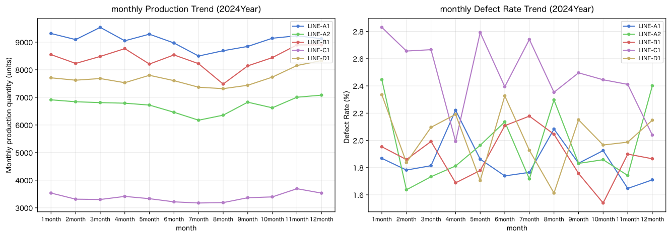

svg

Data overview graph display completed (SVG 1/2)

No.061: Understanding the Concept of Window Functions

Meaning in Practice

window function is an SQL feature that allows you to add aggregate values to each row without aggregating them. While GROUP BY “collapses rows,” window functions “add calculations while holding rows,” which differs.

Examples of use in manufacturing:

While keeping monthly production numbers, the bank is granted a ‘line annual total’ → calculating monthly market shares.
Calculate the ‘cumulative average’ simultaneously while arranging defect rates in chronological order.
Assign the maximum and minimum defect rates of your own line to each record for outlier detection.

Approach to Analysis and Modeling

Window function syntax:

\underbrace{\text{function}(\text{column})}_\text{aggregate function}\;\; \underbrace{\text{OVER}\,(\text{PARTITION BY column}\;\;\text{ORDER BY column})}_\text{Window definition}

PARTITION BY is ‘Which group will be calculated’ (abbreviated for the entire line), ORDER BY specifies the “order of rows within the window.”

comparison item	GROUP BY	window function
Number of lines	Decreased after consolidation	Retain as is
exert effort	One line per group	Added calculation values to all rows
How to use	Summary Report	Simultaneous referencing of rows + aggregate values

Check with Python

# No.061: Comparing the differences between GROUP BY and window functions

print('=== GROUP BY: 5Consolidated by line (annual total by line)===')
q(conn, '''
SELECT line_code, factory_name,
       SUM(production_qty) AS annual_prod
FROM   production
GROUP  BY line_code, factory_name
ORDER  BY annual_prod DESC
''')

print()
print('=== window function: 60Adding annual totals and monthly shares while maintaining the line ===')
q(conn, '''
SELECT month,
       line_code,
       production_qty,
       SUM(production_qty) OVER (PARTITION BY line_code)  AS line_annual_prod,
       ROUND(
           production_qty * 100.0 /
           SUM(production_qty) OVER (PARTITION BY line_code),
           1
       )                                                   AS month_share_pct
FROM   production
WHERE  line_code = 'LINE-A1'
ORDER  BY month
''')

=== GROUP BY: Consolidated into 5 lines (annual total by line) ===
── SQL ─────────────────────────────────────────
  SELECT line_code, factory_name,
         SUM(production_qty) AS annual_prod
  FROM   production
  GROUP  BY line_code, factory_name
  ORDER  BY annual_prod DESC
───────────────────────────────────────────────
shape: (5, 3)
┌───────────┬──────────────┬─────────────┐
│ line_code ┆ factory_name ┆ annual_prod │
│ ---       ┆ ---          ┆ ---         │
│ str       ┆ str          ┆ i64         │
╞═══════════╪══════════════╪═════════════╡
│ LINE-A1   ┆ Tokyo Factory     ┆ 108782      │
│ LINE-B1   ┆ Osaka Factory     ┆ 100853      │
│ LINE-D1   ┆ Fukuoka Factory     ┆ 92289       │
│ LINE-A2   ┆ Tokyo Factory     ┆ 80592       │
│ LINE-C1   ┆ Nagoya Factory   ┆ 40454       │
└───────────┴──────────────┴─────────────┘
↳ Obtained in 5 rows

=== Window Function: Adds annual total and monthly share while holding 60 rows ===
── SQL ─────────────────────────────────────────
  SELECT month,
         line_code,
         production_qty,
         SUM(production_qty) OVER (PARTITION BY line_code)  AS line_annual_prod,
         ROUND(
             production_qty * 100.0 /
             SUM(production_qty) OVER (PARTITION BY line_code),
             1
         )                                                   AS month_share_pct
  FROM   production
  WHERE  line_code = 'LINE-A1'
  ORDER  BY month
───────────────────────────────────────────────
shape: (12, 5)
┌─────────┬───────────┬────────────────┬──────────────────┬─────────────────┐
│ month   ┆ line_code ┆ production_qty ┆ line_annual_prod ┆ month_share_pct │
│ ---     ┆ ---       ┆ ---            ┆ ---              ┆ ---             │
│ str     ┆ str       ┆ i64            ┆ i64              ┆ f64             │
╞═════════╪═══════════╪════════════════╪══════════════════╪═════════════════╡
│ 2024-01 ┆ LINE-A1   ┆ 9314           ┆ 108782           ┆ 8.6             │
│ 2024-02 ┆ LINE-A1   ┆ 9093           ┆ 108782           ┆ 8.4             │
│ 2024-03 ┆ LINE-A1   ┆ 9536           ┆ 108782           ┆ 8.8             │
│ 2024-04 ┆ LINE-A1   ┆ 9050           ┆ 108782           ┆ 8.3             │
│ 2024-05 ┆ LINE-A1   ┆ 9289           ┆ 108782           ┆ 8.5             │
│ …       ┆ …         ┆ …              ┆ …                ┆ …               │
│ 2024-08 ┆ LINE-A1   ┆ 8690           ┆ 108782           ┆ 8.0             │
│ 2024-09 ┆ LINE-A1   ┆ 8845           ┆ 108782           ┆ 8.1             │
│ 2024-10 ┆ LINE-A1   ┆ 9142           ┆ 108782           ┆ 8.4             │
│ 2024-11 ┆ LINE-A1   ┆ 9231           ┆ 108782           ┆ 8.5             │
│ 2024-12 ┆ LINE-A1   ┆ 9125           ┆ 108782           ┆ 8.4             │
└─────────┴───────────┴────────────────┴──────────────────┴─────────────────┘
↳ Obtained in 12 lines

shape: (12, 5)

month	line_code	production_qty	line_annual_prod	month_share_pct
str	str	i64	i64	f64
”2024-01"	"LINE-A1”	9314	108782	8.6
”2024-02"	"LINE-A1”	9093	108782	8.4
”2024-03"	"LINE-A1”	9536	108782	8.8
”2024-04"	"LINE-A1”	9050	108782	8.3
”2024-05"	"LINE-A1”	9289	108782	8.5
…	…	…	…	…
“2024-08"	"LINE-A1”	8690	108782	8.0
”2024-09"	"LINE-A1”	8845	108782	8.1
”2024-10"	"LINE-A1”	9142	108782	8.4
”2024-11"	"LINE-A1”	9231	108782	8.5
”2024-12"	"LINE-A1”	9125	108782	8.4

Reading the results

GROUP BY aggregates 5 lines × 12 months = 60 rows of data into 5 lines. Monthly breakdowns are lost.
The window function retains 12 lines (12 months of LINE-A1), Add line_annual_prod (annual total) and month_share_pct (monthly share) to each row
Looking at month_share_pct, the production share slightly declines during the summer (July to August) You can check individual data for each month while reviewing it. Insights that GROUP BY cannot obtain

No.062: Consecutive Numbers in ROW_NUMBER

Meaning in Practice

ROW_NUMBER() Unique serial number each line. Even if the same value (tie) exists, There will always be a different number (the order depends on ORDER BY).

Examples of use in manufacturing:

Identifying the ‘Top 3 Months with Low Production on Each Line’ and Using It to Review Production Expansion Plans
Refer to ‘Nth Event’ by adding chronological numbers to the test record
Split and acquire large volumes of data through data paging (WHERE rn BETWEEN 11 AND 20)

Approach to Analysis and Modeling

ROW_NUMBER() is often used for filtering through external queries (such as subqueries or CTEs).

SELECT * FROM (
    SELECT *, ROW_NUMBER() OVER (PARTITION BY line_code ORDER BY production_qty ASC) AS rn
    FROM production
) WHERE rn <= 3   -- Months with low production volume on each line TOP3

\text{ROW\_NUMBER} = 1, 2, 3, \ldots \quad (\text{Even if the value is the same, the number always differs})

Check with Python

# No.062: ROW_NUMBER — Identifying Months with Low Production on Each Line

print('=== Months with low production volume on each line TOP3（ROW_NUMBER）===')
q(conn, '''
SELECT month, line_code, factory_name, production_qty,
       defect_qty,
       ROUND(defect_qty * 100.0 / production_qty, 2) AS dr_pct,
       ROW_NUMBER() OVER (
           PARTITION BY line_code
           ORDER BY production_qty ASC
       ) AS rn
FROM   production
ORDER  BY line_code, rn
LIMIT  15
''')

print()
print('=== With subqueries, rn <= 2 Narrow down (each line Worst production volume2ヶmonth)===')
q(conn, '''
SELECT month, line_code, factory_name, production_qty, dr_pct
FROM (
    SELECT month, line_code, factory_name, production_qty,
           ROUND(defect_qty * 100.0 / production_qty, 2) AS dr_pct,
           ROW_NUMBER() OVER (
               PARTITION BY line_code
               ORDER BY production_qty ASC
           ) AS rn
    FROM   production
)
WHERE  rn <= 2
ORDER  BY line_code, production_qty
''')

=== Top 3 Months with Low Production Volume on Each Line (ROW_NUMBER) ===
── SQL ─────────────────────────────────────────
  SELECT month, line_code, factory_name, production_qty,
         defect_qty,
         ROUND(defect_qty * 100.0 / production_qty, 2) AS dr_pct,
         ROW_NUMBER() OVER (
             PARTITION BY line_code
             ORDER BY production_qty ASC
         ) AS rn
  FROM   production
  ORDER  BY line_code, rn
  LIMIT  15
───────────────────────────────────────────────
shape: (15, 7)
┌─────────┬───────────┬──────────────┬────────────────┬────────────┬────────┬─────┐
│ month   ┆ line_code ┆ factory_name ┆ production_qty ┆ defect_qty ┆ dr_pct ┆ rn  │
│ ---     ┆ ---       ┆ ---          ┆ ---            ┆ ---        ┆ ---    ┆ --- │
│ str     ┆ str       ┆ str          ┆ i64            ┆ i64        ┆ f64    ┆ i64 │
╞═════════╪═══════════╪══════════════╪════════════════╪════════════╪════════╪═════╡
│ 2024-07 ┆ LINE-A1   ┆ Tokyo Factory     ┆ 8497           ┆ 150        ┆ 1.77   ┆ 1   │
│ 2024-08 ┆ LINE-A1   ┆ Tokyo Factory     ┆ 8690           ┆ 181        ┆ 2.08   ┆ 2   │
│ 2024-09 ┆ LINE-A1   ┆ Tokyo Factory     ┆ 8845           ┆ 162        ┆ 1.83   ┆ 3   │
│ 2024-06 ┆ LINE-A1   ┆ Tokyo Factory     ┆ 8970           ┆ 156        ┆ 1.74   ┆ 4   │
│ 2024-04 ┆ LINE-A1   ┆ Tokyo Factory     ┆ 9050           ┆ 201        ┆ 2.22   ┆ 5   │
│ …       ┆ …         ┆ …            ┆ …              ┆ …          ┆ …      ┆ …   │
│ 2024-01 ┆ LINE-A1   ┆ Tokyo Factory     ┆ 9314           ┆ 174        ┆ 1.87   ┆ 11  │
│ 2024-03 ┆ LINE-A1   ┆ Tokyo Factory     ┆ 9536           ┆ 173        ┆ 1.81   ┆ 12  │
│ 2024-07 ┆ LINE-A2   ┆ Tokyo Factory     ┆ 6173           ┆ 106        ┆ 1.72   ┆ 1   │
│ 2024-08 ┆ LINE-A2   ┆ Tokyo Factory     ┆ 6355           ┆ 146        ┆ 2.3    ┆ 2   │
│ 2024-06 ┆ LINE-A2   ┆ Tokyo Factory     ┆ 6460           ┆ 138        ┆ 2.14   ┆ 3   │
└─────────┴───────────┴──────────────┴────────────────┴────────────┴────────┴─────┘
↳ Obtained in 15 rows

=== Narrow down to rn <= 2 by subquery (lowest production quantity per line in 2 months) ===
── SQL ─────────────────────────────────────────
  SELECT month, line_code, factory_name, production_qty, dr_pct
  FROM (
      SELECT month, line_code, factory_name, production_qty,
             ROUND(defect_qty * 100.0 / production_qty, 2) AS dr_pct,
             ROW_NUMBER() OVER (
                 PARTITION BY line_code
                 ORDER BY production_qty ASC
             ) AS rn
      FROM   production
  )
  WHERE  rn <= 2
  ORDER  BY line_code, production_qty
───────────────────────────────────────────────
shape: (10, 5)
┌─────────┬───────────┬──────────────┬────────────────┬────────┐
│ month   ┆ line_code ┆ factory_name ┆ production_qty ┆ dr_pct │
│ ---     ┆ ---       ┆ ---          ┆ ---            ┆ ---    │
│ str     ┆ str       ┆ str          ┆ i64            ┆ f64    │
╞═════════╪═══════════╪══════════════╪════════════════╪════════╡
│ 2024-07 ┆ LINE-A1   ┆ Tokyo Factory     ┆ 8497           ┆ 1.77   │
│ 2024-08 ┆ LINE-A1   ┆ Tokyo Factory     ┆ 8690           ┆ 2.08   │
│ 2024-07 ┆ LINE-A2   ┆ Tokyo Factory     ┆ 6173           ┆ 1.72   │
│ 2024-08 ┆ LINE-A2   ┆ Tokyo Factory     ┆ 6355           ┆ 2.3    │
│ 2024-08 ┆ LINE-B1   ┆ Osaka Factory     ┆ 7482           ┆ 2.04   │
│ 2024-09 ┆ LINE-B1   ┆ Osaka Factory     ┆ 8141           ┆ 1.76   │
│ 2024-07 ┆ LINE-C1   ┆ Nagoya Factory   ┆ 3174           ┆ 2.74   │
│ 2024-08 ┆ LINE-C1   ┆ Nagoya Factory   ┆ 3188           ┆ 2.35   │
│ 2024-08 ┆ LINE-D1   ┆ Fukuoka Factory     ┆ 7315           ┆ 1.61   │
│ 2024-07 ┆ LINE-D1   ┆ Fukuoka Factory     ┆ 7368           ┆ 1.93   │
└─────────┴───────────┴──────────────┴────────────────┴────────┘
↳ Obtained in 10 lines

shape: (10, 5)

month	line_code	factory_name	production_qty	dr_pct
str	str	str	i64	f64
”2024-07"	"LINE-A1"	"Tokyo Factory”	8497	1.77
”2024-08"	"LINE-A1"	"Tokyo Factory”	8690	2.08
”2024-07"	"LINE-A2"	"Tokyo Factory”	6173	1.72
”2024-08"	"LINE-A2"	"Tokyo Factory”	6355	2.3
”2024-08"	"LINE-B1"	"Osaka Factory”	7482	2.04
”2024-09"	"LINE-B1"	"Osaka Factory”	8141	1.76
”2024-07"	"LINE-C1"	"Nagoya Factory”	3174	2.74
”2024-08"	"LINE-C1"	"Nagoya Factory”	3188	2.35
”2024-08"	"LINE-D1"	"Fukuoka Factory”	7315	1.61
”2024-07"	"LINE-D1"	"Fukuoka Factory”	7368	1.93

Reading the results

PARTITION BY line_code assigns an independent serial number to each line. Starting from the months with the lowest production volume on the line, from 1st, 2nd, 3rd, … and so the numbers are assigned.
By filtering with WHERE rn <= 2, you can find the ‘worst production months by line’ You can list them all. We will also check the defect rates (dr_pct) for these months
If there is a tendency for ‘months with low production yields higher defect rates,’ It is necessary to review process management during downtime declines.

No.063: Create Rankings with RANK

Meaning in Practice

RANK() same ranking the same value (tie) and jump to the next rank. It’s the same as in sports report cards: ‘If there are multiple tied runners-up, the next is fourth place.’

Examples of use in manufacturing:

Creating a monthly defect rate ranking for all lines × and quantifying improvement priorities
Track the changes in each line’s position over time using monthly production volume rankings.
Incorporating factory-specific quality KPI rankings into monthly reports

Approach to Analysis and Modeling

\text{RANK}:\quad \underbrace{2.5\%}_{\text{1 bit}},\ \underbrace{2.0\%,\; 2.0\%}_{\text{2 bits, 2 bits (tie)}},\ \underbrace{1.8\%}_{\text{4th place} \leftarrow \text{skip 3rd place}}

If there are many ties, the rankings of the following teams can jump significantly. If continuity in the ranking is important, use DENSE_RANK (No.064).

Check with Python

# No.063: RANK — Defect rate ranking for all lines × all months

print('=== All Lines × Full month Defect rate ranking (RANK higher rank10Item)===')
q(conn, '''
SELECT month,
       line_code,
       factory_name,
       production_qty,
       defect_qty,
       ROUND(defect_qty * 100.0 / production_qty, 2) AS dr_pct,
       RANK() OVER (
           ORDER BY defect_qty * 1.0 / production_qty DESC
       ) AS dr_rank
FROM   production
ORDER  BY dr_rank
LIMIT  10
''')

print()
print('=== LINE-A1 Monthly defect rate rankings within LINE ===')
q(conn, '''
SELECT month, line_code,
       ROUND(defect_qty * 100.0 / production_qty, 2) AS dr_pct,
       RANK() OVER (
           PARTITION BY line_code
           ORDER BY defect_qty * 1.0 / production_qty DESC
       ) AS monthly_dr_rank
FROM   production
WHERE  line_code = 'LINE-A1'
ORDER  BY monthly_dr_rank
''')

=== All Lines × Monthly Defect Rate Ranking (Top 10 RANK) ===
── SQL ─────────────────────────────────────────
  SELECT month,
         line_code,
         factory_name,
         production_qty,
         defect_qty,
         ROUND(defect_qty * 100.0 / production_qty, 2) AS dr_pct,
         RANK() OVER (
             ORDER BY defect_qty * 1.0 / production_qty DESC
         ) AS dr_rank
  FROM   production
  ORDER  BY dr_rank
  LIMIT  10
───────────────────────────────────────────────
shape: (10, 7)
┌─────────┬───────────┬──────────────┬────────────────┬────────────┬────────┬─────────┐
│ month   ┆ line_code ┆ factory_name ┆ production_qty ┆ defect_qty ┆ dr_pct ┆ dr_rank │
│ ---     ┆ ---       ┆ ---          ┆ ---            ┆ ---        ┆ ---    ┆ ---     │
│ str     ┆ str       ┆ str          ┆ i64            ┆ i64        ┆ f64    ┆ i64     │
╞═════════╪═══════════╪══════════════╪════════════════╪════════════╪════════╪═════════╡
│ 2024-01 ┆ LINE-C1   ┆ Nagoya Factory   ┆ 3534           ┆ 100        ┆ 2.83   ┆ 1       │
│ 2024-05 ┆ LINE-C1   ┆ Nagoya Factory   ┆ 3331           ┆ 93         ┆ 2.79   ┆ 2       │
│ 2024-07 ┆ LINE-C1   ┆ Nagoya Factory   ┆ 3174           ┆ 87         ┆ 2.74   ┆ 3       │
│ 2024-03 ┆ LINE-C1   ┆ Nagoya Factory   ┆ 3301           ┆ 88         ┆ 2.67   ┆ 4       │
│ 2024-02 ┆ LINE-C1   ┆ Nagoya Factory   ┆ 3313           ┆ 88         ┆ 2.66   ┆ 5       │
│ 2024-09 ┆ LINE-C1   ┆ Nagoya Factory   ┆ 3365           ┆ 84         ┆ 2.5    ┆ 6       │
│ 2024-01 ┆ LINE-A2   ┆ Tokyo Factory     ┆ 6910           ┆ 169        ┆ 2.45   ┆ 7       │
│ 2024-10 ┆ LINE-C1   ┆ Nagoya Factory   ┆ 3395           ┆ 83         ┆ 2.44   ┆ 8       │
│ 2024-11 ┆ LINE-C1   ┆ Nagoya Factory   ┆ 3692           ┆ 89         ┆ 2.41   ┆ 9       │
│ 2024-12 ┆ LINE-A2   ┆ Tokyo Factory     ┆ 7081           ┆ 170        ┆ 2.4    ┆ 10      │
└─────────┴───────────┴──────────────┴────────────────┴────────────┴────────┴─────────┘
↳ Obtained in 10 lines

=== Monthly defect rate ranking within LINE focused on LINE-A1 ===
── SQL ─────────────────────────────────────────
  SELECT month, line_code,
         ROUND(defect_qty * 100.0 / production_qty, 2) AS dr_pct,
         RANK() OVER (
             PARTITION BY line_code
             ORDER BY defect_qty * 1.0 / production_qty DESC
         ) AS monthly_dr_rank
  FROM   production
  WHERE  line_code = 'LINE-A1'
  ORDER  BY monthly_dr_rank
───────────────────────────────────────────────
shape: (12, 4)
┌─────────┬───────────┬────────┬─────────────────┐
│ month   ┆ line_code ┆ dr_pct ┆ monthly_dr_rank │
│ ---     ┆ ---       ┆ ---    ┆ ---             │
│ str     ┆ str       ┆ f64    ┆ i64             │
╞═════════╪═══════════╪════════╪═════════════════╡
│ 2024-04 ┆ LINE-A1   ┆ 2.22   ┆ 1               │
│ 2024-08 ┆ LINE-A1   ┆ 2.08   ┆ 2               │
│ 2024-10 ┆ LINE-A1   ┆ 1.93   ┆ 3               │
│ 2024-01 ┆ LINE-A1   ┆ 1.87   ┆ 4               │
│ 2024-05 ┆ LINE-A1   ┆ 1.86   ┆ 5               │
│ …       ┆ …         ┆ …      ┆ …               │
│ 2024-02 ┆ LINE-A1   ┆ 1.78   ┆ 8               │
│ 2024-07 ┆ LINE-A1   ┆ 1.77   ┆ 9               │
│ 2024-06 ┆ LINE-A1   ┆ 1.74   ┆ 10              │
│ 2024-12 ┆ LINE-A1   ┆ 1.71   ┆ 11              │
│ 2024-11 ┆ LINE-A1   ┆ 1.65   ┆ 12              │
└─────────┴───────────┴────────┴─────────────────┘
↳ Obtained in 12 lines

shape: (12, 4)

month	line_code	dr_pct	monthly_dr_rank
str	str	f64	i64
”2024-04"	"LINE-A1”	2.22	1
”2024-08"	"LINE-A1”	2.08	2
”2024-10"	"LINE-A1”	1.93	3
”2024-01"	"LINE-A1”	1.87	4
”2024-05"	"LINE-A1”	1.86	5
…	…	…	…
“2024-02"	"LINE-A1”	1.78	8
”2024-07"	"LINE-A1”	1.77	9
”2024-06"	"LINE-A1”	1.74	10
”2024-12"	"LINE-A1”	1.71	11
”2024-11"	"LINE-A1”	1.65	12

Reading the results

The record for top defect rate (dr_rank = 1) has reached LINE-C1 (Nagoya Plant, shock absorbers) If it is concentrated, priority investment in quality improvement on this line is justified
Check your line’s worst month by ranking (PARTITION BY line_code) within your LINE By identifying them, it becomes the starting point for investigating “what happened in which month and what happened.”
If a tie occurs, the next number is skipped in RANK. If this behavior is an issue, use DENSE_RANK from No.064

No.064: Handling tied rankings in DENSE_RANK

Meaning in Practice

DENSE_RANK() gives the same ranking to the tie, Since the next ranking is Do not fly (the difference from RANK), Filtering for “within rank N” is intuitive.

Examples of use in manufacturing:

When extracting the monthly line × the top 5 defect rates, you want to avoid rankings where there is no 4th place.
When selecting the target of the improvement program as the ‘Lower N Group,’ the number of groups remains fixed
When treating lines with the same KPI value as the same ‘improvement stage’

Approach to Analysis and Modeling

\text{RANK vs DENSE\_RANK}

Score	RANK()	DENSE_RANK()
2.5% (maximum defect rate)	1	1
2.0% (tied)	2	2
2.0% (tied)	2	2
1.8%	4 ← 3Skip	3 ← continuous

In DENSE_RANK, there is no situation where “no third place exists.”

Check with Python

# No.064: Checking the difference between DENSE_RANK vs RANK

print('=== Examples of Usage: If you have a tie, RANK vs DENSE_RANK ===')
q(conn, '''
WITH example(line, dr) AS (
    VALUES ('LINE-C1（2.6%）', 2.6),
           ('LINE-D1（2.2%）', 2.2),
           ('LINE-A2（2.1%）', 2.1),
           ('LINE-B1（2.0%）', 2.0),
           ('LINE-A1（2.0%）', 2.0),
           ('LINE-XX（1.9%）', 1.9)
)
SELECT line, dr,
       RANK()       OVER (ORDER BY dr DESC) AS rank_result,
       DENSE_RANK() OVER (ORDER BY dr DESC) AS dense_rank_result
FROM   example
''')

print()
print('=== Real Data: Full month Defect rate ROUND(1digit) Ranking comparison when rounded ===')
q(conn, '''
SELECT month, line_code,
       ROUND(defect_qty * 100.0 / production_qty, 1) AS dr_pct_1dec,
       RANK()       OVER (ORDER BY ROUND(defect_qty * 100.0 / production_qty, 1) DESC) AS rnk,
       DENSE_RANK() OVER (ORDER BY ROUND(defect_qty * 100.0 / production_qty, 1) DESC) AS dense_rnk
FROM   production
ORDER  BY dr_pct_1dec DESC
LIMIT  15
''')

=== Explanation Example: RANK vs DENSE_RANK When There Are Ties ===
── SQL ─────────────────────────────────────────
  WITH example(line, dr) AS (
      VALUES ('LINE-C1（2.6%）', 2.6),
             ('LINE-D1（2.2%）', 2.2),
             ('LINE-A2（2.1%）', 2.1),
             ('LINE-B1（2.0%）', 2.0),
             ('LINE-A1（2.0%）', 2.0),
             ('LINE-XX（1.9%）', 1.9)
  )
  SELECT line, dr,
         RANK()       OVER (ORDER BY dr DESC) AS rank_result,
         DENSE_RANK() OVER (ORDER BY dr DESC) AS dense_rank_result
  FROM   example
───────────────────────────────────────────────
shape: (6, 4)
┌─────────────────┬─────┬─────────────┬───────────────────┐
│ line            ┆ dr  ┆ rank_result ┆ dense_rank_result │
│ ---             ┆ --- ┆ ---         ┆ ---               │
│ str             ┆ f64 ┆ i64         ┆ i64               │
╞═════════════════╪═════╪═════════════╪═══════════════════╡
│ LINE-C1（2.6%） ┆ 2.6 ┆ 1           ┆ 1                 │
│ LINE-D1（2.2%） ┆ 2.2 ┆ 2           ┆ 2                 │
│ LINE-A2（2.1%） ┆ 2.1 ┆ 3           ┆ 3                 │
│ LINE-B1（2.0%） ┆ 2.0 ┆ 4           ┆ 4                 │
│ LINE-A1（2.0%） ┆ 2.0 ┆ 4           ┆ 4                 │
│ LINE-XX（1.9%） ┆ 1.9 ┆ 6           ┆ 5                 │
└─────────────────┴─────┴─────────────┴───────────────────┘
↳ Get in 6 lines

=== Real Data: Ranking Comparison When Defect Rates Round by ROUND (Single Digit) ===
── SQL ─────────────────────────────────────────
  SELECT month, line_code,
         ROUND(defect_qty * 100.0 / production_qty, 1) AS dr_pct_1dec,
         RANK()       OVER (ORDER BY ROUND(defect_qty * 100.0 / production_qty, 1) DESC) AS rnk,
         DENSE_RANK() OVER (ORDER BY ROUND(defect_qty * 100.0 / production_qty, 1) DESC) AS dense_rnk
  FROM   production
  ORDER  BY dr_pct_1dec DESC
  LIMIT  15
───────────────────────────────────────────────
shape: (15, 5)
┌─────────┬───────────┬─────────────┬─────┬───────────┐
│ month   ┆ line_code ┆ dr_pct_1dec ┆ rnk ┆ dense_rnk │
│ ---     ┆ ---       ┆ ---         ┆ --- ┆ ---       │
│ str     ┆ str       ┆ f64         ┆ i64 ┆ i64       │
╞═════════╪═══════════╪═════════════╪═════╪═══════════╡
│ 2024-01 ┆ LINE-C1   ┆ 2.8         ┆ 1   ┆ 1         │
│ 2024-05 ┆ LINE-C1   ┆ 2.8         ┆ 1   ┆ 1         │
│ 2024-02 ┆ LINE-C1   ┆ 2.7         ┆ 3   ┆ 2         │
│ 2024-03 ┆ LINE-C1   ┆ 2.7         ┆ 3   ┆ 2         │
│ 2024-07 ┆ LINE-C1   ┆ 2.7         ┆ 3   ┆ 2         │
│ …       ┆ …         ┆ …           ┆ …   ┆ …         │
│ 2024-11 ┆ LINE-C1   ┆ 2.4         ┆ 7   ┆ 4         │
│ 2024-12 ┆ LINE-A2   ┆ 2.4         ┆ 7   ┆ 4         │
│ 2024-01 ┆ LINE-D1   ┆ 2.3         ┆ 13  ┆ 5         │
│ 2024-06 ┆ LINE-D1   ┆ 2.3         ┆ 13  ┆ 5         │
│ 2024-08 ┆ LINE-A2   ┆ 2.3         ┆ 13  ┆ 5         │
└─────────┴───────────┴─────────────┴─────┴───────────┘
↳ Obtained in 15 rows

shape: (15, 5)

month	line_code	dr_pct_1dec	rnk	dense_rnk
str	str	f64	i64	i64
”2024-01"	"LINE-C1”	2.8	1	1
”2024-05"	"LINE-C1”	2.8	1	1
”2024-02"	"LINE-C1”	2.7	3	2
”2024-03"	"LINE-C1”	2.7	3	2
”2024-07"	"LINE-C1”	2.7	3	2
…	…	…	…	…
“2024-11"	"LINE-C1”	2.4	7	4
”2024-12"	"LINE-A2”	2.4	7	4
”2024-01"	"LINE-D1”	2.3	13	5
”2024-06"	"LINE-D1”	2.3	13	5
”2024-08"	"LINE-A2”	2.3	13	5

Reading the results

In the explanatory example, when LINE-B1 and LINE-A1 have a tie rate of 2.0%, RANK() then adds 4rank (skipping 3). DENSE_RANK() then adds 3rank (continuous)
Using ROUND(..., 1) in real data makes tie-rate situations more likely, You can check the actual differences in behavior between the two functions
If you have a policy of “focusing improvement investments on the top 3 lines,” Extracting with DENSE_RANK <= 3 may contain more lines than RANK. Choosing according to business requirements is important

No.065: Extracting the Top Loss Threshold

Meaning in Practice

ROW_NUMBER() OVER (PARTITION BY ... ORDER BY ...) The pattern for extracting Top Rankings by Category (Factory) N rows is: This is one of the most practical uses of SQL window functions.

Examples of use in manufacturing:

Identify the worst defect loss threshold for each factory with a single query
Extracting top and bottom quality lines by category (subcategory)
Tracking the line with the largest production volume increase and decrease every month

Approach to Analysis and Modeling

The amount of defective loss is calculated based on unit price × number of defects.

\text{Bad Loss Amount} = \sum_{t=1}^{12} \text{defect\_qty}_t \times \text{unit\_price}

High-priced parts (crankshaft ¥8,500 / shock absorber ¥2,800) Even if the number of defects is small, the loss amount can be large. Loss Amount Based rankings directly influence management decisions.

Check with Python

# No.065: Extracting the Worst Defect Loss Amount by Factory by ROW_NUMBER Line

print('=== annual Defective Loss Amount & Production Value (Aggregated by Line)===')
q(conn, '''
WITH annual AS (
    SELECT line_code, factory_id, factory_name, part_name, unit_price,
           SUM(production_qty)              AS annual_prod,
           SUM(defect_qty)                  AS annual_defect,
           SUM(production_qty * unit_price) AS production_value,
           SUM(defect_qty    * unit_price)  AS defect_loss
    FROM   production
    GROUP  BY line_code, factory_id, factory_name, part_name, unit_price
),
ranked AS (
    SELECT *,
           ROW_NUMBER() OVER (
               PARTITION BY factory_id
               ORDER BY defect_loss DESC
           ) AS rn
    FROM   annual
)
SELECT factory_id, factory_name, line_code, part_name, unit_price,
       annual_prod, annual_defect, production_value, defect_loss, rn
FROM   ranked
ORDER  BY defect_loss DESC
''')

print()
print('=== By Factory Worst1Line (rn = 1）===')
q(conn, '''
WITH annual AS (
    SELECT line_code, factory_id, factory_name, part_name, unit_price,
           SUM(defect_qty * unit_price) AS defect_loss
    FROM   production
    GROUP  BY line_code, factory_id, factory_name, part_name, unit_price
),
ranked AS (
    SELECT *,
           ROW_NUMBER() OVER (PARTITION BY factory_id ORDER BY defect_loss DESC) AS rn
    FROM   annual
)
SELECT factory_id, factory_name, line_code, part_name, defect_loss
FROM   ranked
WHERE  rn = 1
ORDER  BY defect_loss DESC
''')

=== Annual Defect Loss Amount & Production Value (Summary by Line) ===
── SQL ─────────────────────────────────────────
  WITH annual AS (
      SELECT line_code, factory_id, factory_name, part_name, unit_price,
             SUM(production_qty)              AS annual_prod,
             SUM(defect_qty)                  AS annual_defect,
             SUM(production_qty * unit_price) AS production_value,
             SUM(defect_qty    * unit_price)  AS defect_loss
      FROM   production
      GROUP  BY line_code, factory_id, factory_name, part_name, unit_price
  ),
  ranked AS (
      SELECT *,
             ROW_NUMBER() OVER (
                 PARTITION BY factory_id
                 ORDER BY defect_loss DESC
             ) AS rn
      FROM   annual
  )
  SELECT factory_id, factory_name, line_code, part_name, unit_price,
         annual_prod, annual_defect, production_value, defect_loss, rn
  FROM   ranked
  ORDER  BY defect_loss DESC
───────────────────────────────────────────────
shape: (5, 10)
┌────────────┬────────────┬───────────┬────────────┬───┬────────────┬────────────┬───────────┬─────┐
│ factory_id ┆ factory_na ┆ line_code ┆ part_name  ┆ … ┆ annual_def ┆ production ┆ defect_lo ┆ rn  │
│ ---        ┆ me         ┆ ---       ┆ ---        ┆   ┆ ect        ┆ _value     ┆ ss        ┆ --- │
│ str        ┆ ---        ┆ str       ┆ str        ┆   ┆ ---        ┆ ---        ┆ ---       ┆ i64 │
│            ┆ str        ┆           ┆            ┆   ┆ i64        ┆ i64        ┆ i64       ┆     │
╞════════════╪════════════╪═══════════╪════════════╪═══╪════════════╪════════════╪═══════════╪═════╡
│ F04        ┆ Fukuoka Factory   ┆ LINE-D1   ┆ Cranksy ┆ … ┆ 1869       ┆ 784456500  ┆ 15886500  ┆ 1   │
│            ┆            ┆           ┆ Yaft     ┆   ┆            ┆            ┆           ┆     │
│ F03        ┆ Nagoya Factory ┆ LINE-C1   ┆ shock a ┆ … ┆ 1004       ┆ 113271200  ┆ 2811200   ┆ 1   │
│            ┆            ┆           ┆ busoba   ┆   ┆            ┆            ┆           ┆     │
│ F01        ┆ Tokyo Factory   ┆ LINE-A1   ┆ Piston ri ┆ … ┆ 2016       ┆ 130538400  ┆ 2419200   ┆ 1   │
│            ┆            ┆           ┆ Ng       ┆   ┆            ┆            ┆           ┆     │
│ F02        ┆ Osaka Factory   ┆ LINE-B1   ┆ Piston ri ┆ … ┆ 1903       ┆ 121023600  ┆ 2283600   ┆ 1   │
│            ┆            ┆           ┆ Ng       ┆   ┆            ┆            ┆           ┆     │
│ F01        ┆ Tokyo Factory   ┆ LINE-A2   ┆ brake pad ┆ … ┆ 1584       ┆ 76562400   ┆ 1504800   ┆ 2   │
│            ┆            ┆           ┆ Dd       ┆   ┆            ┆            ┆           ┆     │
└────────────┴────────────┴───────────┴────────────┴───┴────────────┴────────────┴───────────┴─────┘
↳ Obtained in 5 rows

=== Worst 1 Line by Factory (rn = 1) ===
── SQL ─────────────────────────────────────────
  WITH annual AS (
      SELECT line_code, factory_id, factory_name, part_name, unit_price,
             SUM(defect_qty * unit_price) AS defect_loss
      FROM   production
      GROUP  BY line_code, factory_id, factory_name, part_name, unit_price
  ),
  ranked AS (
      SELECT *,
             ROW_NUMBER() OVER (PARTITION BY factory_id ORDER BY defect_loss DESC) AS rn
      FROM   annual
  )
  SELECT factory_id, factory_name, line_code, part_name, defect_loss
  FROM   ranked
  WHERE  rn = 1
  ORDER  BY defect_loss DESC
───────────────────────────────────────────────
shape: (4, 5)
┌────────────┬──────────────┬───────────┬────────────────────┬─────────────┐
│ factory_id ┆ factory_name ┆ line_code ┆ part_name          ┆ defect_loss │
│ ---        ┆ ---          ┆ ---       ┆ ---                ┆ ---         │
│ str        ┆ str          ┆ str       ┆ str                ┆ i64         │
╞════════════╪══════════════╪═══════════╪════════════════════╪═════════════╡
│ F04        ┆ Fukuoka Factory     ┆ LINE-D1   ┆ Crankshaft   ┆ 15886500    │
│ F03        ┆ Nagoya Factory   ┆ LINE-C1   ┆ shock absorber ┆ 2811200     │
│ F01        ┆ Tokyo Factory     ┆ LINE-A1   ┆ piston ring     ┆ 2419200     │
│ F02        ┆ Osaka Factory     ┆ LINE-B1   ┆ piston ring     ┆ 2283600     │
└────────────┴──────────────┴───────────┴────────────────────┴─────────────┘
↳ Obtained in 4 lines

shape: (4, 5)

factory_id	factory_name	line_code	part_name	defect_loss
str	str	str	str	i64
”F04"	"Fukuoka Factory"	"LINE-D1"	"Crankshaft”	15886500
”F03"	"Nagoya Factory"	"LINE-C1"	"shock absorber”	2811200
”F01"	"Tokyo Factory"	"LINE-A1"	"piston ring”	2419200
”F02"	"Osaka Factory"	"LINE-B1"	"piston ring”	2283600

Reading the results

The LINE-D1 (Fukuoka Factory, Crankshaft ¥8,500) has a moderate defect rate, It is The amount of loss loss is overwhelmingly large. because the unit price is the highest. By using the “Loss Amount Ranking” instead of the “Defect Quantity Ranking,” You can prioritize solutions directly linked to management impact.
The F01 (Tokyo factory) has two lines (LINE-A1, LINE-A2), PARTITION BY factory_id in-factory rankings work effectively
ROW_NUMBER() ... WHERE rn = 1 pattern is: “Getting only one representative row per category” is the most general-purpose SQL technique

No.066: Creating Production Volume Rankings by Line

Meaning in Practice

By including multiple RANK() or DENSE_RANK() in the same query, You can calculate multiple KPI Composite ranking all at once.

Examples of use in manufacturing:

Simultaneous display of production volume ranking (higher is better) and defect rate ranking (lower is better)
Identifying lines with “high production volume but poor quality” and lines with “low production volume but good quality”
Evaluate well-balanced lines with composite scores (e.g., production rank + quality rank)

Approach to Analysis and Modeling

Ranking analysis combining two KPIs Visualize the Trade-off of decision-making.

\text{composite score} = w_1 \cdot \text{rank}(\text{production}) + w_2 \cdot \text{rank}(\text{quality})

Weight $w_1, w_2$ is adjusted according to management policies (whether quantity or quality). In this exercise, we use a simple total rank of $w_1 = w_2 = 1$ .

Check with Python

# No.066: Combined evaluation of annual production volume ranking × defect rate ranking

print('=== By Line Production Volume Ranking × Quality Ranking (Composite Evaluation)===')
q(conn, '''
WITH totals AS (
    SELECT line_code, factory_name, part_name,
           SUM(production_qty)                                      AS annual_prod,
           SUM(defect_qty)                                          AS annual_defect,
           ROUND(SUM(defect_qty) * 100.0 / SUM(production_qty), 2) AS annual_dr,
           SUM(defect_qty * unit_price)                             AS defect_loss
    FROM   production
    GROUP  BY line_code, factory_name, part_name
)
SELECT line_code, factory_name, part_name,
       annual_prod, annual_defect, annual_dr, defect_loss,
       RANK() OVER (ORDER BY annual_prod DESC) AS prod_rank,
       RANK() OVER (ORDER BY annual_dr   ASC)  AS quality_rank,
       RANK() OVER (ORDER BY annual_prod DESC) +
       RANK() OVER (ORDER BY annual_dr   ASC)  AS composite_rank
FROM   totals
ORDER  BY composite_rank ASC
''')

=== Production Volume Ranking by Line × Quality Ranking (Composite Evaluation) ===
── SQL ─────────────────────────────────────────
  WITH totals AS (
      SELECT line_code, factory_name, part_name,
             SUM(production_qty)                                      AS annual_prod,
             SUM(defect_qty)                                          AS annual_defect,
             ROUND(SUM(defect_qty) * 100.0 / SUM(production_qty), 2) AS annual_dr,
             SUM(defect_qty * unit_price)                             AS defect_loss
      FROM   production
      GROUP  BY line_code, factory_name, part_name
  )
  SELECT line_code, factory_name, part_name,
         annual_prod, annual_defect, annual_dr, defect_loss,
         RANK() OVER (ORDER BY annual_prod DESC) AS prod_rank,
         RANK() OVER (ORDER BY annual_dr   ASC)  AS quality_rank,
         RANK() OVER (ORDER BY annual_prod DESC) +
         RANK() OVER (ORDER BY annual_dr   ASC)  AS composite_rank
  FROM   totals
  ORDER  BY composite_rank ASC
───────────────────────────────────────────────
shape: (5, 10)
┌───────────┬───────────┬───────────┬───────────┬───┬───────────┬───────────┬───────────┬──────────┐
│ line_code ┆ factory_n ┆ part_name ┆ annual_pr ┆ … ┆ defect_lo ┆ prod_rank ┆ quality_r ┆ composit │
│ ---       ┆ ame       ┆ ---       ┆ od        ┆   ┆ ss        ┆ ---       ┆ ank       ┆ e_rank   │
│ str       ┆ ---       ┆ str       ┆ ---       ┆   ┆ ---       ┆ i64       ┆ ---       ┆ ---      │
│           ┆ str       ┆           ┆ i64       ┆   ┆ i64       ┆           ┆ i64       ┆ i64      │
╞═══════════╪═══════════╪═══════════╪═══════════╪═══╪═══════════╪═══════════╪═══════════╪══════════╡
│ LINE-A1   ┆ Tokyo Factory  ┆ piston  ┆ 108782    ┆ … ┆ 2419200   ┆ 1         ┆ 1         ┆ 2        │
│           ┆           ┆ Ring    ┆           ┆   ┆           ┆           ┆           ┆          │
│ LINE-B1   ┆ Osaka Factory  ┆ piston  ┆ 100853    ┆ … ┆ 2283600   ┆ 2         ┆ 2         ┆ 4        │
│           ┆           ┆ Ring    ┆           ┆   ┆           ┆           ┆           ┆          │
│ LINE-D1   ┆ Fukuoka Factory  ┆ crank  ┆ 92289     ┆ … ┆ 15886500  ┆ 3         ┆ 4         ┆ 7        │
│           ┆           ┆ shaft  ┆           ┆   ┆           ┆           ┆           ┆          │
│ LINE-A2   ┆ Tokyo Factory  ┆ Brakes  ┆ 80592     ┆ … ┆ 1504800   ┆ 4         ┆ 3         ┆ 7        │
│           ┆           ┆ Pad    ┆           ┆   ┆           ┆           ┆           ┆          │
│ LINE-C1   ┆ Nagoya Technical  ┆ shock  ┆ 40454     ┆ … ┆ 2811200   ┆ 5         ┆ 5         ┆ 10       │
│           ┆ Venue        ┆ Absau  ┆           ┆   ┆           ┆           ┆           ┆          │
│           ┆           ┆ ba        ┆           ┆   ┆           ┆           ┆           ┆          │
└───────────┴───────────┴───────────┴───────────┴───┴───────────┴───────────┴───────────┴──────────┘
↳ Obtained in 5 rows

shape: (5, 10)

line_code	factory_name	part_name	annual_prod	annual_defect	annual_dr	defect_loss	prod_rank	quality_rank	composite_rank
str	str	str	i64	i64	f64	i64	i64	i64	i64
”LINE-A1"	"Tokyo Factory"	"piston ring”	108782	2016	1.85	2419200	1	1	2
”LINE-B1"	"Osaka Factory"	"piston ring”	100853	1903	1.89	2283600	2	2	4
”LINE-D1"	"Fukuoka Factory"	"Crankshaft”	92289	1869	2.03	15886500	3	4	7
”LINE-A2"	"Tokyo Factory"	"brake pad”	80592	1584	1.97	1504800	4	3	7
”LINE-C1"	"Nagoya Factory"	"shock absorber”	40454	1004	2.48	2811200	5	5	10

Reading the results

prod_rank (production volume ranking) and quality_rank (defect rate ranking) By displaying them simultaneously, you can instantly see the trade-off between quantity and quality
composite_rank (Composite Score: Total Rank) is a low line, We achieve a balance in both production volume and quality.
The line with “High production volume ranking, low quality ranking” Prioritizing mass production at the expense of quality may be the issue. Review equipment and processes, and consider the priority of quality engineer assignments

No.067: Retrieve the previous value with LAG

Meaning in Practice

LAG(columns, N) retrieves the value from the current line by the previous N lines. By splitting it with PARTITION BY, you can accurately reference the “previous month’s value within the line.”

Examples of use in manufacturing:

Display this month’s production figures and last month’s production numbers in a single row to track changes
Comparing this month’s defect rate with last month’s rate to confirm improvement trends
Detecting short-term trends compared to the value from two months ago (LAG(col, 2))

Approach to Analysis and Modeling

LAG is used as a preprocessing for “line difference calculation.”

\Delta x_t = x_t - \underbrace{x_{t-1}}_{\text{LAG}(x,\, 1)}

In time series analysis, to ensure this difference is stationarity, It is also used (as shown in the I(1) difference of the ARIMA model).

In monthly production management, this is an essential operation as the basis for calculating ‘month-on-month’ results.

Check with Python

# No.067: LAG — Retrieves last month's production and defect rates in the same row

print('=== LINE-A1: By month Production Volume and Defect Rate And Previous Month Value ===')
q(conn, '''
WITH base AS (
    SELECT month, line_code, factory_name, production_qty,
           ROUND(defect_qty * 100.0 / production_qty, 2) AS dr_pct
    FROM   production
    WHERE  line_code = 'LINE-A1'
)
SELECT month, line_code, production_qty, dr_pct,
       LAG(production_qty, 1) OVER (ORDER BY month) AS prev_prod,
       LAG(dr_pct,          1) OVER (ORDER BY month) AS prev_dr
FROM   base
ORDER  BY month
''')

print()
print('=== All Lines: Previous month's price included (PARTITION BY line_code See by line for details)===')
q(conn, '''
WITH base AS (
    SELECT month, line_code, production_qty,
           ROUND(defect_qty * 100.0 / production_qty, 2) AS dr_pct
    FROM   production
)
SELECT month, line_code, production_qty, dr_pct,
       LAG(production_qty, 1) OVER (PARTITION BY line_code ORDER BY month) AS prev_prod,
       LAG(dr_pct,          1) OVER (PARTITION BY line_code ORDER BY month) AS prev_dr
FROM   base
ORDER  BY line_code, month
LIMIT  15
''')

=== LINE-A1: Monthly Production Quantity, Defect Rate, and Previous Month Values ===
── SQL ─────────────────────────────────────────
  WITH base AS (
      SELECT month, line_code, factory_name, production_qty,
             ROUND(defect_qty * 100.0 / production_qty, 2) AS dr_pct
      FROM   production
      WHERE  line_code = 'LINE-A1'
  )
  SELECT month, line_code, production_qty, dr_pct,
         LAG(production_qty, 1) OVER (ORDER BY month) AS prev_prod,
         LAG(dr_pct,          1) OVER (ORDER BY month) AS prev_dr
  FROM   base
  ORDER  BY month
───────────────────────────────────────────────
shape: (12, 6)
┌─────────┬───────────┬────────────────┬────────┬───────────┬─────────┐
│ month   ┆ line_code ┆ production_qty ┆ dr_pct ┆ prev_prod ┆ prev_dr │
│ ---     ┆ ---       ┆ ---            ┆ ---    ┆ ---       ┆ ---     │
│ str     ┆ str       ┆ i64            ┆ f64    ┆ i64       ┆ f64     │
╞═════════╪═══════════╪════════════════╪════════╪═══════════╪═════════╡
│ 2024-01 ┆ LINE-A1   ┆ 9314           ┆ 1.87   ┆ null      ┆ null    │
│ 2024-02 ┆ LINE-A1   ┆ 9093           ┆ 1.78   ┆ 9314      ┆ 1.87    │
│ 2024-03 ┆ LINE-A1   ┆ 9536           ┆ 1.81   ┆ 9093      ┆ 1.78    │
│ 2024-04 ┆ LINE-A1   ┆ 9050           ┆ 2.22   ┆ 9536      ┆ 1.81    │
│ 2024-05 ┆ LINE-A1   ┆ 9289           ┆ 1.86   ┆ 9050      ┆ 2.22    │
│ …       ┆ …         ┆ …              ┆ …      ┆ …         ┆ …       │
│ 2024-08 ┆ LINE-A1   ┆ 8690           ┆ 2.08   ┆ 8497      ┆ 1.77    │
│ 2024-09 ┆ LINE-A1   ┆ 8845           ┆ 1.83   ┆ 8690      ┆ 2.08    │
│ 2024-10 ┆ LINE-A1   ┆ 9142           ┆ 1.93   ┆ 8845      ┆ 1.83    │
│ 2024-11 ┆ LINE-A1   ┆ 9231           ┆ 1.65   ┆ 9142      ┆ 1.93    │
│ 2024-12 ┆ LINE-A1   ┆ 9125           ┆ 1.71   ┆ 9231      ┆ 1.65    │
└─────────┴───────────┴────────────────┴────────┴───────────┴─────────┘
↳ Obtained in 12 lines

=== All lines: Previous month's price (see line by PARTITION BY line_code) ===
── SQL ─────────────────────────────────────────
  WITH base AS (
      SELECT month, line_code, production_qty,
             ROUND(defect_qty * 100.0 / production_qty, 2) AS dr_pct
      FROM   production
  )
  SELECT month, line_code, production_qty, dr_pct,
         LAG(production_qty, 1) OVER (PARTITION BY line_code ORDER BY month) AS prev_prod,
         LAG(dr_pct,          1) OVER (PARTITION BY line_code ORDER BY month) AS prev_dr
  FROM   base
  ORDER  BY line_code, month
  LIMIT  15
───────────────────────────────────────────────
shape: (15, 6)
┌─────────┬───────────┬────────────────┬────────┬───────────┬─────────┐
│ month   ┆ line_code ┆ production_qty ┆ dr_pct ┆ prev_prod ┆ prev_dr │
│ ---     ┆ ---       ┆ ---            ┆ ---    ┆ ---       ┆ ---     │
│ str     ┆ str       ┆ i64            ┆ f64    ┆ i64       ┆ f64     │
╞═════════╪═══════════╪════════════════╪════════╪═══════════╪═════════╡
│ 2024-01 ┆ LINE-A1   ┆ 9314           ┆ 1.87   ┆ null      ┆ null    │
│ 2024-02 ┆ LINE-A1   ┆ 9093           ┆ 1.78   ┆ 9314      ┆ 1.87    │
│ 2024-03 ┆ LINE-A1   ┆ 9536           ┆ 1.81   ┆ 9093      ┆ 1.78    │
│ 2024-04 ┆ LINE-A1   ┆ 9050           ┆ 2.22   ┆ 9536      ┆ 1.81    │
│ 2024-05 ┆ LINE-A1   ┆ 9289           ┆ 1.86   ┆ 9050      ┆ 2.22    │
│ …       ┆ …         ┆ …              ┆ …      ┆ …         ┆ …       │
│ 2024-11 ┆ LINE-A1   ┆ 9231           ┆ 1.65   ┆ 9142      ┆ 1.93    │
│ 2024-12 ┆ LINE-A1   ┆ 9125           ┆ 1.71   ┆ 9231      ┆ 1.65    │
│ 2024-01 ┆ LINE-A2   ┆ 6910           ┆ 2.45   ┆ null      ┆ null    │
│ 2024-02 ┆ LINE-A2   ┆ 6841           ┆ 1.64   ┆ 6910      ┆ 2.45    │
│ 2024-03 ┆ LINE-A2   ┆ 6810           ┆ 1.73   ┆ 6841      ┆ 1.64    │
└─────────┴───────────┴────────────────┴────────┴───────────┴─────────┘
↳ Obtained in 15 rows

shape: (15, 6)

month	line_code	production_qty	dr_pct	prev_prod	prev_dr
str	str	i64	f64	i64	f64
”2024-01"	"LINE-A1”	9314	1.87	null	null
”2024-02"	"LINE-A1”	9093	1.78	9314	1.87
”2024-03"	"LINE-A1”	9536	1.81	9093	1.78
”2024-04"	"LINE-A1”	9050	2.22	9536	1.81
”2024-05"	"LINE-A1”	9289	1.86	9050	2.22
…	…	…	…	…	…
“2024-11"	"LINE-A1”	9231	1.65	9142	1.93
”2024-12"	"LINE-A1”	9125	1.71	9231	1.65
”2024-01"	"LINE-A2”	6910	2.45	null	null
”2024-02"	"LINE-A2”	6841	1.64	6910	2.45
”2024-03"	"LINE-A2”	6810	1.73	6841	1.64

Reading the results

Since there is no previous month’s value for 2024-01, prev_prod/prev_dr is NULL. This correctly represents the absence of data
By using PARTITION BY line_code, you can avoid mixing values between lines, Only the “previous month’s value on the same line” is referenced. If you omit PARTITION BY, the last row of a different line will be used as the previous month’s value
Comparing the defect rate prev_dr with the current month’s dr_pct, This serves as a basis to confirm whether the condition is improved (-) or worsened (+) (calculated using No.068).

No.068: Calculating Month-to-Month Differences

Meaning in Practice

Month-over-month (Month-over-Month = MoM) is the most fundamental fluctuation indicator in production management. By automatically calculating “how much has changed or decreased since the previous month?” This reduces manual update man-hours and enables early detection of abnormal fluctuations.

Examples of use in manufacturing:

Alerts are issued when the month-on-month production percentage exceeds the baseline value (±10%)
Quantitatively evaluate the effectiveness of improvement programs based on the previous month’s change in defect rate (+ or −)
Track production plan achievement rates by yearly cumulative MoM trends

Approach to Analysis and Modeling

Formula for calculating month-on-month comparison and difference from previous month:

\text{Month-over-month (\%)} = \frac{x_t - x_{t-1}}{x_{t-1}} \times 100 \qquad \text{Previous Month} = x_t - x_{t-1}

When the previous month’s value is 0 or NULL, the month-on-month value cannot be defined. CASE WHEN prev IS NOT NULL AND prev > 0 THEN ... ELSE NULL END will handle it.

Check with Python

# No.068: Month-on-month MoM — Calculating monthly production and defect rate month-on-month

print('=== Month-over-month/Month-over-month change (LINE-A1 / LINE-B1 / LINE-D1）===')
df_mom = q(conn, '''
WITH base AS (
    SELECT month, line_code, factory_name,
           production_qty,
           ROUND(defect_qty * 100.0 / production_qty, 2) AS dr_pct
    FROM   production
),
with_lag AS (
    SELECT month, line_code, factory_name, production_qty, dr_pct,
           LAG(production_qty, 1) OVER (PARTITION BY line_code ORDER BY month) AS prev_prod,
           LAG(dr_pct,          1) OVER (PARTITION BY line_code ORDER BY month) AS prev_dr
    FROM   base
)
SELECT month, line_code, production_qty, prev_prod,
       CASE WHEN prev_prod IS NOT NULL
            THEN ROUND((production_qty - prev_prod) * 100.0 / prev_prod, 1)
            ELSE NULL
       END AS mom_pct,
       dr_pct, prev_dr,
       CASE WHEN prev_dr IS NOT NULL
            THEN ROUND(dr_pct - prev_dr, 2)
            ELSE NULL
       END AS dr_diff
FROM   with_lag
WHERE  line_code IN ('LINE-A1', 'LINE-B1', 'LINE-D1')
ORDER  BY line_code, month
''')

=== Month-over-month/Month-on-month change (LINE-A1 / LINE-B1 / LINE-D1) ===
── SQL ─────────────────────────────────────────
  WITH base AS (
      SELECT month, line_code, factory_name,
             production_qty,
             ROUND(defect_qty * 100.0 / production_qty, 2) AS dr_pct
      FROM   production
  ),
  with_lag AS (
      SELECT month, line_code, factory_name, production_qty, dr_pct,
             LAG(production_qty, 1) OVER (PARTITION BY line_code ORDER BY month) AS prev_prod,
             LAG(dr_pct,          1) OVER (PARTITION BY line_code ORDER BY month) AS prev_dr
      FROM   base
  )
  SELECT month, line_code, production_qty, prev_prod,
         CASE WHEN prev_prod IS NOT NULL
              THEN ROUND((production_qty - prev_prod) * 100.0 / prev_prod, 1)
              ELSE NULL
         END AS mom_pct,
         dr_pct, prev_dr,
         CASE WHEN prev_dr IS NOT NULL
              THEN ROUND(dr_pct - prev_dr, 2)
              ELSE NULL
         END AS dr_diff
  FROM   with_lag
  WHERE  line_code IN ('LINE-A1', 'LINE-B1', 'LINE-D1')
  ORDER  BY line_code, month
───────────────────────────────────────────────
shape: (36, 8)
┌─────────┬───────────┬────────────────┬───────────┬─────────┬────────┬─────────┬─────────┐
│ month   ┆ line_code ┆ production_qty ┆ prev_prod ┆ mom_pct ┆ dr_pct ┆ prev_dr ┆ dr_diff │
│ ---     ┆ ---       ┆ ---            ┆ ---       ┆ ---     ┆ ---    ┆ ---     ┆ ---     │
│ str     ┆ str       ┆ i64            ┆ i64       ┆ f64     ┆ f64    ┆ f64     ┆ f64     │
╞═════════╪═══════════╪════════════════╪═══════════╪═════════╪════════╪═════════╪═════════╡
│ 2024-01 ┆ LINE-A1   ┆ 9314           ┆ null      ┆ null    ┆ 1.87   ┆ null    ┆ null    │
│ 2024-02 ┆ LINE-A1   ┆ 9093           ┆ 9314      ┆ -2.4    ┆ 1.78   ┆ 1.87    ┆ -0.09   │
│ 2024-03 ┆ LINE-A1   ┆ 9536           ┆ 9093      ┆ 4.9     ┆ 1.81   ┆ 1.78    ┆ 0.03    │
│ 2024-04 ┆ LINE-A1   ┆ 9050           ┆ 9536      ┆ -5.1    ┆ 2.22   ┆ 1.81    ┆ 0.41    │
│ 2024-05 ┆ LINE-A1   ┆ 9289           ┆ 9050      ┆ 2.6     ┆ 1.86   ┆ 2.22    ┆ -0.36   │
│ …       ┆ …         ┆ …              ┆ …         ┆ …       ┆ …      ┆ …       ┆ …       │
│ 2024-08 ┆ LINE-D1   ┆ 7315           ┆ 7368      ┆ -0.7    ┆ 1.61   ┆ 1.93    ┆ -0.32   │
│ 2024-09 ┆ LINE-D1   ┆ 7438           ┆ 7315      ┆ 1.7     ┆ 2.15   ┆ 1.61    ┆ 0.54    │
│ 2024-10 ┆ LINE-D1   ┆ 7733           ┆ 7438      ┆ 4.0     ┆ 1.97   ┆ 2.15    ┆ -0.18   │
│ 2024-11 ┆ LINE-D1   ┆ 8153           ┆ 7733      ┆ 5.4     ┆ 1.99   ┆ 1.97    ┆ 0.02    │
│ 2024-12 ┆ LINE-D1   ┆ 8334           ┆ 8153      ┆ 2.2     ┆ 2.15   ┆ 1.99    ┆ 0.16    │
└─────────┴───────────┴────────────────┴───────────┴─────────┴────────┴─────────┴─────────┘
↳ Obtained in 36 rows

# No.068 Visualization: Monthly Production MoM (Month-on-Month) Trends (3 Lines)
TARGET_LINES = ['LINE-A1', 'LINE-B1', 'LINE-D1']
COLORS_3     = ['#4878CF', '#D65F5F', '#C4AD66']
MONTHS_LBL   = [f'{m+1}month' for m in range(12)]

# Obtain monthly production numbers and MoM per line
prod_data = {lc: [] for lc in TARGET_LINES}
mom_data  = {lc: [] for lc in TARGET_LINES}

for row in df_mom.to_dicts():
    if row['line_code'] in TARGET_LINES:
        prod_data[row['line_code']].append(row['production_qty'])
        mom_data[row['line_code']].append(row['mom_pct'])

fig, axes = plt.subplots(1, 2, figsize=(14, 5))

# Left: Monthly production trends (line lines)
ax1 = axes[0]
for lc, col in zip(TARGET_LINES, COLORS_3):
    ax1.plot(range(12), prod_data[lc], marker='o', markersize=4,
             linewidth=1.8, color=col, label=lc)
ax1.set_title('monthly Production Volume Trends (2024Year)', fontsize=12, pad=10)
ax1.set_xlabel('month', fontsize=10)
ax1.set_ylabel('Production Quantity (units)', fontsize=10)
ax1.set_xticks(range(12))
ax1.set_xticklabels(MONTHS_LBL, fontsize=8)
ax1.legend(fontsize=8)
ax1.grid(alpha=0.3)

# Right: Bar graph of month-on-month MoM (%) (11 months from February to December 2024)
ax2 = axes[1]
x = range(11)  # 2024-02 to 2024-12
width = 0.27
for i, (lc, col) in enumerate(zip(TARGET_LINES, COLORS_3)):
    vals = mom_data[lc][1:]  # skip 2024-01 (None)
    vals_plot = [v if v is not None else 0 for v in vals]
    bars = ax2.bar([xi + i * width for xi in x], vals_plot, width,
                   color=col, alpha=0.8, label=lc)
ax2.axhline(0, color='black', linewidth=0.8, linestyle='--')
ax2.set_title('Compared to the previous month (MoM %) Trends (2024year2〜12month)', fontsize=12, pad=10)
ax2.set_xlabel('month', fontsize=10)
ax2.set_ylabel('Compared to the previous month (%）', fontsize=10)
ax2.set_xticks([xi + width for xi in x])
ax2.set_xticklabels([f'{m+2}month' for m in range(11)], fontsize=8)
ax2.legend(fontsize=8)
ax2.grid(axis='y', alpha=0.3)

plt.tight_layout()
plt.show()
print('Month-on-month graph display completed (SVG 2/2）')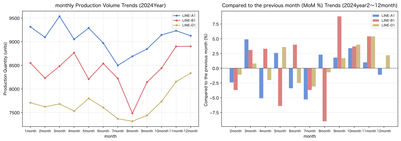

svg

Month-on-month graph display complete (SVG 2/2)

Reading the results

Left Graph: Production volume on each line slightly decreases during the summer (July–August), and by the end of the year (November–December), You can see the increasing seasonality.
Right graph: Months with negative MoM (production decreased compared to the previous month) will be displayed below 0 on the bar graph. A sharp decline (such as -15% or less) may be due to equipment troubles, material shortages, or the impact of consecutive holidays
The line where the defect rate dr_diff is negative (improving) for consecutive months is This is evidence that quality improvement activities are being effective. Conversely, if the positive (worsening) persists, an urgent investigation into the cause is necessary

No.069: Calculating Cumulative Production Volume

Meaning in Practice

SUM() OVER (ORDER BY ... ROWS UNBOUNDED PRECEDING) You can calculate cumulative aggregate (total running). You can calculate the year-end total while maintaining monthly data without using GROUP BY.

Examples of use in manufacturing:

Tracking monthly cumulative achievement and achievement rate against annual production targets (e.g., 100,000 units)
Identify months when cumulative defects exceed the acceptable limit and set alerts
Analyzing long-term equipment trends by comparing cumulative production over multiple years

Approach to Analysis and Modeling

Cumulative tabulation formula:

S_t = \sum_{\tau=1}^{t} x_{\tau} \quad\Leftrightarrow\quad \text{SUM}(x) \text{ OVER } (\text{ORDER BY } t \text{ ROWS UNBOUNDED PRECEDING})

ROWS UNBOUNDED PRECEDING means “all rows before the current line (from the first row to the current line).” As a result, the cumulative value increases monotonically as the month progresses.

Check with Python

# No.069: Calculation of Cumulative Production Volume and Cumulative Defect Loss

print('=== All Lines monthly + Cumulative Production Volume and Cumulative Loss ===')
q(conn, '''
WITH monthly AS (
    SELECT month, line_code, factory_name,
           production_qty,
           defect_qty * unit_price AS defect_loss_monthly
    FROM   production
)
SELECT month, line_code, factory_name,
       production_qty,
       SUM(production_qty) OVER (
           PARTITION BY line_code
           ORDER BY month
           ROWS UNBOUNDED PRECEDING
       )                         AS cumsum_prod,
       defect_loss_monthly,
       SUM(defect_loss_monthly) OVER (
           PARTITION BY line_code
           ORDER BY month
           ROWS UNBOUNDED PRECEDING
       )                         AS cumsum_loss
FROM   monthly
ORDER  BY line_code, month
LIMIT  24
''')

print()
print('=== Annual Goals 100,000 units Cumulative achievement rate (LINE-A1）===')
q(conn, '''
WITH monthly AS (
    SELECT month, production_qty
    FROM   production
    WHERE  line_code = 'LINE-A1'
)
SELECT month,
       production_qty,
       SUM(production_qty) OVER (ORDER BY month ROWS UNBOUNDED PRECEDING) AS cumsum,
       ROUND(
           SUM(production_qty) OVER (ORDER BY month ROWS UNBOUNDED PRECEDING) * 100.0 / 100000,
           1
       ) AS achievement_pct
FROM   monthly
ORDER  BY month
''')

=== All Lines Monthly + Cumulative Production Volume & Cumulative Loss ===
── SQL ─────────────────────────────────────────
  WITH monthly AS (
      SELECT month, line_code, factory_name,
             production_qty,
             defect_qty * unit_price AS defect_loss_monthly
      FROM   production
  )
  SELECT month, line_code, factory_name,
         production_qty,
         SUM(production_qty) OVER (
             PARTITION BY line_code
             ORDER BY month
             ROWS UNBOUNDED PRECEDING
         )                         AS cumsum_prod,
         defect_loss_monthly,
         SUM(defect_loss_monthly) OVER (
             PARTITION BY line_code
             ORDER BY month
             ROWS UNBOUNDED PRECEDING
         )                         AS cumsum_loss
  FROM   monthly
  ORDER  BY line_code, month
  LIMIT  24
───────────────────────────────────────────────
shape: (24, 7)
┌─────────┬───────────┬──────────────┬────────────────┬─────────────┬────────────────┬─────────────┐
│ month   ┆ line_code ┆ factory_name ┆ production_qty ┆ cumsum_prod ┆ defect_loss_mo ┆ cumsum_loss │
│ ---     ┆ ---       ┆ ---          ┆ ---            ┆ ---         ┆ nthly          ┆ ---         │
│ str     ┆ str       ┆ str          ┆ i64            ┆ i64         ┆ ---            ┆ i64         │
│         ┆           ┆              ┆                ┆             ┆ i64            ┆             │
╞═════════╪═══════════╪══════════════╪════════════════╪═════════════╪════════════════╪═════════════╡
│ 2024-01 ┆ LINE-A1   ┆ Tokyo Factory     ┆ 9314           ┆ 9314        ┆ 208800         ┆ 208800      │
│ 2024-02 ┆ LINE-A1   ┆ Tokyo Factory     ┆ 9093           ┆ 18407       ┆ 194400         ┆ 403200      │
│ 2024-03 ┆ LINE-A1   ┆ Tokyo Factory     ┆ 9536           ┆ 27943       ┆ 207600         ┆ 610800      │
│ 2024-04 ┆ LINE-A1   ┆ Tokyo Factory     ┆ 9050           ┆ 36993       ┆ 241200         ┆ 852000      │
│ 2024-05 ┆ LINE-A1   ┆ Tokyo Factory     ┆ 9289           ┆ 46282       ┆ 207600         ┆ 1059600     │
│ …       ┆ …         ┆ …            ┆ …              ┆ …           ┆ …              ┆ …           │
│ 2024-08 ┆ LINE-A2   ┆ Tokyo Factory     ┆ 6355           ┆ 53059       ┆ 138700         ┆ 991800      │
│ 2024-09 ┆ LINE-A2   ┆ Tokyo Factory     ┆ 6826           ┆ 59885       ┆ 118750         ┆ 1110550     │
│ 2024-10 ┆ LINE-A2   ┆ Tokyo Factory     ┆ 6621           ┆ 66506       ┆ 116850         ┆ 1227400     │
│ 2024-11 ┆ LINE-A2   ┆ Tokyo Factory     ┆ 7005           ┆ 73511       ┆ 115900         ┆ 1343300     │
│ 2024-12 ┆ LINE-A2   ┆ Tokyo Factory     ┆ 7081           ┆ 80592       ┆ 161500         ┆ 1504800     │
└─────────┴───────────┴──────────────┴────────────────┴─────────────┴────────────────┴─────────────┘
↳ 24 lines obtained

=== Cumulative Achievement Rate Against Annual Target of 100,000 Items (LINE-A1) ===
── SQL ─────────────────────────────────────────
  WITH monthly AS (
      SELECT month, production_qty
      FROM   production
      WHERE  line_code = 'LINE-A1'
  )
  SELECT month,
         production_qty,
         SUM(production_qty) OVER (ORDER BY month ROWS UNBOUNDED PRECEDING) AS cumsum,
         ROUND(
             SUM(production_qty) OVER (ORDER BY month ROWS UNBOUNDED PRECEDING) * 100.0 / 100000,
             1
         ) AS achievement_pct
  FROM   monthly
  ORDER  BY month
───────────────────────────────────────────────
shape: (12, 4)
┌─────────┬────────────────┬────────┬─────────────────┐
│ month   ┆ production_qty ┆ cumsum ┆ achievement_pct │
│ ---     ┆ ---            ┆ ---    ┆ ---             │
│ str     ┆ i64            ┆ i64    ┆ f64             │
╞═════════╪════════════════╪════════╪═════════════════╡
│ 2024-01 ┆ 9314           ┆ 9314   ┆ 9.3             │
│ 2024-02 ┆ 9093           ┆ 18407  ┆ 18.4            │
│ 2024-03 ┆ 9536           ┆ 27943  ┆ 27.9            │
│ 2024-04 ┆ 9050           ┆ 36993  ┆ 37.0            │
│ 2024-05 ┆ 9289           ┆ 46282  ┆ 46.3            │
│ …       ┆ …              ┆ …      ┆ …               │
│ 2024-08 ┆ 8690           ┆ 72439  ┆ 72.4            │
│ 2024-09 ┆ 8845           ┆ 81284  ┆ 81.3            │
│ 2024-10 ┆ 9142           ┆ 90426  ┆ 90.4            │
│ 2024-11 ┆ 9231           ┆ 99657  ┆ 99.7            │
│ 2024-12 ┆ 9125           ┆ 108782 ┆ 108.8           │
└─────────┴────────────────┴────────┴─────────────────┘
↳ Obtained in 12 lines

shape: (12, 4)

month	production_qty	cumsum	achievement_pct
str	i64	i64	f64
”2024-01”	9314	9314	9.3
”2024-02”	9093	18407	18.4
”2024-03”	9536	27943	27.9
”2024-04”	9050	36993	37.0
”2024-05”	9289	46282	46.3
…	…	…	…
“2024-08”	8690	72439	72.4
”2024-09”	8845	81284	81.3
”2024-10”	9142	90426	90.4
”2024-11”	9231	99657	99.7
”2024-12”	9125	108782	108.8

Reading the results

cumsum_prod increases monotonously as the month progresses. Even in summer months of declining production (months with month-on-month decline), the cumulative amount continues to increase, You can track the gap from your annual goals on a monthly basis.
cumsum_loss (cumulative non-performing loss amount) is increasing at the fastest rate. Early quality improvement interventions are necessary. You can get a monthly outlook for total losses over the year
Since you can check your achievement_pct (achievement rate) monthly, It becomes easier to predict “If we keep this pace, what is the year-end achievement rate?”

No.070: Calculating the Moving Average

Meaning in Practice

moving average (Moving Average) is a method that continuously calculates the average over the most recent N months, Extracting trends by removing short-term noise monthly data.

Examples of use in manufacturing:

Distinguishing “temporary spikes” and “true quality degradation” by the 3-month moving average defect rate
Understand long-term trends by removing seasonal fluctuations with the 6-month moving average production quantity
Using months with large discrepancies between moving averages and actual performance as anomaly detection signals

Approach to Analysis and Modeling

$n$ Definition of the Monthly Moving Average:

\text{MA}_n(t) = \frac{1}{n} \sum_{\tau=t-n+1}^{t} x_{\tau}

Implementation in SQL:

AVG(x) OVER (
    PARTITION BY line_code
    ORDER BY month
    ROWS BETWEEN (n-1) PRECEDING AND CURRENT ROW
)

ROWS BETWEEN 2 PRECEDING AND CURRENT ROW targets “current row + previous 2 lines” = 3 lines.

Check with Python

# No.070: Calculation of 3-Month and 6-Month Moving Average Non-Performing Rate

print('=== monthly non-performing rate + 3ヶmonth / 6ヶmonth Moving Average (LINE-A1, LINE-C1）===')
q(conn, '''
WITH monthly AS (
    SELECT month, line_code, factory_name,
           ROUND(defect_qty * 100.0 / production_qty, 3) AS dr_pct
    FROM   production
)
SELECT month, line_code, factory_name, dr_pct,
       ROUND(AVG(dr_pct) OVER (
           PARTITION BY line_code
           ORDER BY month
           ROWS BETWEEN 2 PRECEDING AND CURRENT ROW
       ), 3) AS ma3,
       ROUND(AVG(dr_pct) OVER (
           PARTITION BY line_code
           ORDER BY month
           ROWS BETWEEN 5 PRECEDING AND CURRENT ROW
       ), 3) AS ma6
FROM   monthly
WHERE  line_code IN ('LINE-A1', 'LINE-C1')
ORDER  BY line_code, month
''')

print()
print('=== Actual Values and3ヶMonths with large monthly moving average deviations (|separation| > 0.1%）===')
q(conn, '''
WITH monthly AS (
    SELECT month, line_code,
           ROUND(defect_qty * 100.0 / production_qty, 3) AS dr_pct
    FROM   production
),
with_ma AS (
    SELECT month, line_code, dr_pct,
           ROUND(AVG(dr_pct) OVER (
               PARTITION BY line_code
               ORDER BY month
               ROWS BETWEEN 2 PRECEDING AND CURRENT ROW
           ), 3) AS ma3
    FROM   monthly
)
SELECT month, line_code, dr_pct, ma3,
       ROUND(ABS(dr_pct - ma3), 3) AS deviation
FROM   with_ma
WHERE  ABS(dr_pct - ma3) > 0.1
ORDER  BY deviation DESC
LIMIT  10
''')

=== Monthly Non-Performing Rate + 3-Month / 6-Month Moving Average (LINE-A1, LINE-C1) ===
── SQL ─────────────────────────────────────────
  WITH monthly AS (
      SELECT month, line_code, factory_name,
             ROUND(defect_qty * 100.0 / production_qty, 3) AS dr_pct
      FROM   production
  )
  SELECT month, line_code, factory_name, dr_pct,
         ROUND(AVG(dr_pct) OVER (
             PARTITION BY line_code
             ORDER BY month
             ROWS BETWEEN 2 PRECEDING AND CURRENT ROW
         ), 3) AS ma3,
         ROUND(AVG(dr_pct) OVER (
             PARTITION BY line_code
             ORDER BY month
             ROWS BETWEEN 5 PRECEDING AND CURRENT ROW
         ), 3) AS ma6
  FROM   monthly
  WHERE  line_code IN ('LINE-A1', 'LINE-C1')
  ORDER  BY line_code, month
───────────────────────────────────────────────


shape: (24, 6)
┌─────────┬───────────┬──────────────┬────────┬───────┬───────┐
│ month   ┆ line_code ┆ factory_name ┆ dr_pct ┆ ma3   ┆ ma6   │
│ ---     ┆ ---       ┆ ---          ┆ ---    ┆ ---   ┆ ---   │
│ str     ┆ str       ┆ str          ┆ f64    ┆ f64   ┆ f64   │
╞═════════╪═══════════╪══════════════╪════════╪═══════╪═══════╡
│ 2024-01 ┆ LINE-A1   ┆ Tokyo Factory     ┆ 1.868  ┆ 1.868 ┆ 1.868 │
│ 2024-02 ┆ LINE-A1   ┆ Tokyo Factory     ┆ 1.782  ┆ 1.825 ┆ 1.825 │
│ 2024-03 ┆ LINE-A1   ┆ Tokyo Factory     ┆ 1.814  ┆ 1.821 ┆ 1.821 │
│ 2024-04 ┆ LINE-A1   ┆ Tokyo Factory     ┆ 2.221  ┆ 1.939 ┆ 1.921 │
│ 2024-05 ┆ LINE-A1   ┆ Tokyo Factory     ┆ 1.862  ┆ 1.966 ┆ 1.909 │
│ …       ┆ …         ┆ …            ┆ …      ┆ …     ┆ …     │
│ 2024-08 ┆ LINE-C1   ┆ Nagoya Factory   ┆ 2.353  ┆ 2.496 ┆ 2.49  │
│ 2024-09 ┆ LINE-C1   ┆ Nagoya Factory   ┆ 2.496  ┆ 2.53  ┆ 2.461 │
│ 2024-10 ┆ LINE-C1   ┆ Nagoya Factory   ┆ 2.445  ┆ 2.431 ┆ 2.537 │
│ 2024-11 ┆ LINE-C1   ┆ Nagoya Factory   ┆ 2.411  ┆ 2.451 ┆ 2.473 │
│ 2024-12 ┆ LINE-C1   ┆ Nagoya Factory   ┆ 2.039  ┆ 2.298 ┆ 2.414 │
└─────────┴───────────┴──────────────┴────────┴───────┴───────┘
↳ 24 lines obtained

=== Months with a Large Divergence Between Actual Figures and the 3-Month Moving Average (|Deviation| > 0.1%）===
── SQL ─────────────────────────────────────────
  WITH monthly AS (
      SELECT month, line_code,
             ROUND(defect_qty * 100.0 / production_qty, 3) AS dr_pct
      FROM   production
  ),
  with_ma AS (
      SELECT month, line_code, dr_pct,
             ROUND(AVG(dr_pct) OVER (
                 PARTITION BY line_code
                 ORDER BY month
                 ROWS BETWEEN 2 PRECEDING AND CURRENT ROW
             ), 3) AS ma3
      FROM   monthly
  )
  SELECT month, line_code, dr_pct, ma3,
         ROUND(ABS(dr_pct - ma3), 3) AS deviation
  FROM   with_ma
  WHERE  ABS(dr_pct - ma3) > 0.1
  ORDER  BY deviation DESC
  LIMIT  10
───────────────────────────────────────────────
shape: (10, 5)
┌─────────┬───────────┬────────┬───────┬───────────┐
│ month   ┆ line_code ┆ dr_pct ┆ ma3   ┆ deviation │
│ ---     ┆ ---       ┆ ---    ┆ ---   ┆ ---       │
│ str     ┆ str       ┆ f64    ┆ f64   ┆ f64       │
╞═════════╪═══════════╪════════╪═══════╪═══════════╡
│ 2024-04 ┆ LINE-C1   ┆ 1.992  ┆ 2.438 ┆ 0.446     │
│ 2024-02 ┆ LINE-A2   ┆ 1.637  ┆ 2.042 ┆ 0.405     │
│ 2024-12 ┆ LINE-A2   ┆ 2.401  ┆ 2.0   ┆ 0.401     │
│ 2024-08 ┆ LINE-D1   ┆ 1.613  ┆ 1.956 ┆ 0.343     │
│ 2024-05 ┆ LINE-C1   ┆ 2.792  ┆ 2.483 ┆ 0.309     │
│ 2024-05 ┆ LINE-D1   ┆ 1.705  ┆ 1.997 ┆ 0.292     │
│ 2024-04 ┆ LINE-A1   ┆ 2.221  ┆ 1.939 ┆ 0.282     │
│ 2024-12 ┆ LINE-C1   ┆ 2.039  ┆ 2.298 ┆ 0.259     │
│ 2024-09 ┆ LINE-D1   ┆ 2.151  ┆ 1.897 ┆ 0.254     │
│ 2024-06 ┆ LINE-D1   ┆ 2.327  ┆ 2.074 ┆ 0.253     │
└─────────┴───────────┴────────┴───────┴───────────┘
↳ Obtained in 10 lines

shape: (10, 5)

month	line_code	dr_pct	ma3	deviation
str	str	f64	f64	f64
”2024-04"	"LINE-C1”	1.992	2.438	0.446
”2024-02"	"LINE-A2”	1.637	2.042	0.405
”2024-12"	"LINE-A2”	2.401	2.0	0.401
”2024-08"	"LINE-D1”	1.613	1.956	0.343
”2024-05"	"LINE-C1”	2.792	2.483	0.309
”2024-05"	"LINE-D1”	1.705	1.997	0.292
”2024-04"	"LINE-A1”	2.221	1.939	0.282
”2024-12"	"LINE-C1”	2.039	2.298	0.259
”2024-09"	"LINE-D1”	2.151	1.897	0.254
”2024-06"	"LINE-D1”	2.327	2.074	0.253

Reading the results

ma3 (3-month moving average) mitigates fluctuations when the monthly non-performing ratio spikes. In the case of ma3 > dr_pct, this month means the average has improved over the past three months
ma6 (6-month moving average) more strongly removes seasonal fluctuations, Suitable for understanding long-term trends (improvement or deterioration over the year)
Months with a large deviation (actual vs. 3-month MA) are suspected to be Abnormal fluctuations in processes. By setting this as an alert threshold, you can achieve Automatic Monitoring in quality control

Practical Implications Seen Through Target Exercise

Through the window functions learned in No.061–070, you can perform the following manufacturing KPI analysis in a single query.

Practical KPIs	SQL Patterns
Monthly Production Share	`SUM() OVER (PARTITION BY line)`
Identifying the Worst Production Month	`ROW_NUMBER() + WHERE rn <= N`
Defect Rate Rankings	`RANK() / DENSE_RANK() OVER (ORDER BY dr DESC)`
Worst Line by Factory	`ROW_NUMBER() OVER (PARTITION BY factory ORDER BY loss DESC)`
Month-on-month (MoM) %)	`LAG(prod, 1)` → `(prod - prev_prod) / prev_prod * 100`
Cumulative Production Volume and Cumulative Loss	`SUM() OVER (ORDER BY month ROWS UNBOUNDED PRECEDING)`
Defect Rate Moving Average (Noise Removal)	`AVG(dr) OVER (ROWS BETWEEN N PRECEDING AND CURRENT ROW)`

GROUP BY Well then,1Query impossible: “Aggregating while holding rows” analysis, You can freely manipulate them using window functions.

What is necessary for practical implementation

1. Check the database version for window function support

Window functions can be used on SQLite 3.28.0 or later, PostgreSQL 8.4 or later, and MySQL 8.0 or later. The SQLite I used in this notebook is 3.39.0+, and RIGHT JOIN has been added, Almost all standard window functions are available.

2. Performance Optimization

Since window functions tend to perform full table scans, For large data, set an index on the key column of PARTITION BY. CREATE INDEX idx_prod_line ON production(line_code, month);

3. Thorough NULL Handling

If the previous month’s value obtained in LAG() is NULL (first month), Month-on-month calculations are protected in CASE WHEN prev IS NOT NULL THEN ... ELSE NULL END. Treating NULL as zero results in incorrect month-over-month changes (such as -100%).

4. Combination with CTE

Complex window function queries are broken down step-by-step using CTE (WITH clauses), Maintainability is greatly improved. Please utilize the CTE + window function pattern shown in No.069–070.

Conclusion

In this chapter, we will use SQL window functions We analyzed the monthly production KPIs of the manufacturing line from multiple perspectives.

exercise	Main Functions and Syntax	Key Points for Use in Manufacturing
No.061	Basic Structure of `OVER()`	Differences from GROUP BY & Monthly Share Calculation
No.062	`ROW_NUMBER()`	Identify the worst production months for each line by serial number.
No.063	`RANK()`	Defect rate rankings for all lines × all months
No.064	`DENSE_RANK()`	Consecutive numbers assigned in tie rankings
No.065	`ROW_NUMBER() PARTITION BY`	Extraction of Worst Loss Lines by Factory
No.066	`RANK()` Multiple simultaneous applications	Composite ranking of production volume × quality
No.067	`LAG(col, 1)`	Refer to the bank for last month’s production numbers and defect rates
No.068	LAG + CASE	Monthly month-over-month (MoM %) and automatic calculation of the month-over-month difference in defect rate
No.069	`SUM() OVER (ROWS UNBOUNDED PRECEDING)`	Tracking monthly cumulative production volume and cumulative loss
No.070	`AVG() OVER (ROWS BETWEEN N PRECEDING)`	Noise removal and trend extraction with moving averages

In the next chapter (Chapter 8: Practical Data Analysis SQL), You will learn practical queries such as KPI aggregation, RFM analysis, and inventory management that combine these technologies.

Consultations for Corporations

Please feel free to consult us about data analysis, SQL education, and DX promotion in manufacturing using the information below.

📩 Contact Us: surikobo.co.jp/contact Please feel free to consult us first.

Analyze monthly trends on manufacturing lines from multiple perspectives using SQL window functions

Analyze monthly trends on manufacturing lines from multiple perspectives using SQL window functions

SQL 100 Exercises Chapter 7 (No.061–No.070): Window Functions

Introduction: Practical Challenges in Manufacturing Covered in This Article

Common situations on site

Why is this issue so difficult to judge?

1. Understanding the structure of the OVER() phrase

2. Differences Between RANK and DENSE_RANK

3. Default values and NULL handling of LAG / LEAD

4. Frame specification (ROWS vs RANGE)

Overview of Exercise covered this time

Preparing the Python environment

Creation of Fictional Data

No.061: Understanding the Concept of Window Functions

Meaning in Practice

Approach to Analysis and Modeling

Check with Python

Reading the results

No.062: Consecutive Numbers in ROW_NUMBER

Meaning in Practice

Approach to Analysis and Modeling

Check with Python

Reading the results

No.063: Create Rankings with RANK

Meaning in Practice

Approach to Analysis and Modeling

Check with Python

Reading the results

No.064: Handling tied rankings in DENSE_RANK

Meaning in Practice

Approach to Analysis and Modeling

Check with Python

Reading the results

No.065: Extracting the Top Loss Threshold

Meaning in Practice

Approach to Analysis and Modeling

Check with Python

Reading the results

No.066: Creating Production Volume Rankings by Line

Meaning in Practice

Approach to Analysis and Modeling

Check with Python

Reading the results

No.067: Retrieve the previous value with LAG

Meaning in Practice

Approach to Analysis and Modeling

Check with Python

Reading the results

No.068: Calculating Month-to-Month Differences

Meaning in Practice

Approach to Analysis and Modeling

Check with Python

Reading the results

No.069: Calculating Cumulative Production Volume

Meaning in Practice

Approach to Analysis and Modeling

Check with Python

Reading the results

No.070: Calculating the Moving Average

Meaning in Practice

Approach to Analysis and Modeling

Check with Python

Reading the results

Practical Implications Seen Through Target Exercise

What is necessary for practical implementation

1. Check the database version for window function support

2. Performance Optimization

3. Thorough NULL Handling

4. Combination with CTE

Conclusion

Consultations for Corporations

Related Posts

Integrating data quality management, SQL design, and BI integration into production line operations

Deepening manufacturing decision-making with SQL application analysis techniques

Automate order KPIs, customer analysis, and inventory risk assessment using SQL

Automating abnormality detection and KPI aggregation on production lines with subqueries and CTE

Perform cross-analysis of factory, parts, and inspection records using SQL JOINs