100 Exercises / SQL / 100 Exercise-Ups to SQL for Data Analysis

Perform cross-analysis of factory, parts, and inspection records using SQL JOINs

2020-01-10

Perform cross-analysis of factory, parts, and inspection records using SQL JOINs

SQL 100 Exercises Chapter 5 (No.041–No.050): Table Join with JOIN

This article is No.5chapter in the “100 Exercises for SQL Basics for Data Analysis” series. In Chapter 4 (No.031–040), we learned about dates, strings, and calculations. In this chapter, we use JOIN(Table binding) to analyze factory masters, production lines, component masters, and inspection records. We aggregate and analyze data cross-sectionally. We will also practice automatic detection methods for data inconsistencies.

[!NOTE] This material is a notebook previously used by Surikoubo (or personally by the representative, Kazuyama), and has been reconstructed, edited, and published with the company’s permission. All data listed is fictional and has no relation whatsoever to real companies, factories, or figures.

Introduction: Practical Challenges in Manufacturing Covered in This Article

This is a challenge Mr. Watanabe from the IT and Data Management Department at an automotive parts manufacturer.

Consistency verification and cross-sectional analysis of manufacturing performance database data (monthly regular work)
  1. Check whether the inspection record database factory_id/part_code exists in each master table.
  2. Combine factory master × inspection records to aggregate production KPIs by line and factory
  3. Combine parts master × inspection records to calculate defect loss amounts for each part.
  4. Identify parts and factories without inspection records and set master maintenance priorities

Currently, I am comparing master Excel files with performance CSVs using VLOOKUP, As data increases, processing becomes heavier, leading to missed responses.

By using JOIN in SQL, the matching of multiple tables can be completed in 1query, Automatic detection of inconsistent data is also possible.

Common situations on site

Scene	Current Challenges	What SQL JOIN can solve
Summary of Results by Factory	Factory code → Factory name conversion manually done with VLOOKUP	Automatically assign factory names to `INNER JOIN factories`
Calculation of Loss Amount for Parts	Manage unit price tables and performance tables separately	`JOIN parts` Combine unit prices to calculate the loss amount
Identification of Uninspected Parts	Manually check by comparing the master and achievements	Automatic extraction with `LEFT JOIN ... WHERE IS NULL`
Detecting Malicious Code	Visually check whether the code for the achievement data exists in the master	Automatic detection by `LEFT JOIN ... WHERE IS NULL`
Joining three or more tables	Combining multiple VLOOKUPs to complicate	Chain multiple `JOIN` and solve it in a single query

JOIN is a core skill for Data Quality Management and KPI cross-sectional analysis in manufacturing.

Why is this issue so difficult to judge?

Here are four points that JOIN beginners often stumble over.

1. Distinguishing Between INNER JOIN and LEFT JOIN

-- INNER JOIN: Only data matching both tables is retrieved (mismatches excluded)
SELECT * FROM inspections INNER JOIN parts ON inspections.part_code = parts.part_code;

-- LEFT JOIN: Hold all rows in the left table (if there is no match in the right table, NULL）
SELECT * FROM parts LEFT JOIN inspections ON parts.part_code = inspections.part_code;

INNER JOIN is used when you want to aggregate only data that exists reliably. LEFT JOIN is used when you want to detect data that doesn’t exist (master maintenance or quality control).

2. Increase in line count due to duplicate combination keys

If multiple keys of the same key exist in the destination table, the number of rows after joining increases. It is important to always check the number of merging events before and after COUNT(*).

3. Use `IS NULL` to determine NULL

The joined sequence of rows that did not match in LEFT JOIN becomes NULL. WHERE joined_col = NULL is always FALSE. Always use WHERE joined_col IS NULL.

4. Verification of Number of Cases Before and After Joining

If the number of cases differs from expectations, it may be due to duplicate merging keys, NULL, or master inconsistency. Check step by step in SELECT COUNT(*) FROM ....

Overview of Exercise covered this time

No.	Titles	Applications in manufacturing
041	Join tables with INNER JOIN	Inspection Records × Basic Integration of Factory Masters
042	Join one table based on LEFT JOIN	Identifying factories with zero inspection records based on all factories
043	Understanding the RIGHT JOIN Concept	Understanding the equivalence relationship with LEFT JOIN
044	Integrating factory master and inspection records	Aggregation of Results with Factory Name and Regional Information
045	Combining the part master with inspection records	Calculation of loss amount with unit price information attached
046	Join multiple tables	Four-table cross-table analysis: factory + line + parts + inspection records
047	Pay attention to duplicate binding keys	Tracking Increase in Number of Rows Due to Duplicate Quality Standards Tables
048	Confirm the increase in the number of cases after merging	Ensuring data quality through verification of number of transactions before and after JOIN
049	Extracting parts without inspection records	Identifying uninspected parts and prioritizing master maintenance
050	Detecting inspection records that do not exist in the component master	Detection of Malicious Codes and Data Quality Management

Preparing the Python environment

import subprocess, sys
res = subprocess.run(["sw_vers", "-productVersion"], capture_output=True, text=True)
print(f"macOS : {res.stdout.strip()}")
print(f"Python: {sys.version}")

macOS : 26.3
Python: 3.13.1 (main, Dec  3 2024, 17:59:52) [Clang 16.0.0 (clang-1600.0.26.4)]

import sqlite3
import numpy as np
import polars as pl
import matplotlib
import matplotlib.pyplot as plt
from matplotlib.patches import Patch

matplotlib.rcParams['font.family'] = 'Hiragino Maru Gothic Pro'
%config InlineBackend.figure_format = 'svg'
np.random.seed(42)

print(f"sqlite3   : {sqlite3.sqlite_version}")
print(f"polars    : {pl.__version__}")
print(f"numpy     : {np.__version__}")
print(f"matplotlib: {matplotlib.__version__}")
print()
print("Library loading complete")

sqlite3   : 3.47.2
polars    : 1.42.1
numpy     : 2.5.1
matplotlib: 3.11.0

Library loading complete

Creation of Fictional Data

Scenario: Automotive parts manufacturer manufacturing record database / Data Management Department Table Structure: 5 tables

Table Name	number of cases	Description
`factories`	5 items	Factory master (F05: Sendai Factory has no inspection record)
`lines`	8 items	Line master (factory code held as FK)
`parts`	8 items	Parts master (BRK-002 / ELC-002 / SUS-002 have no inspection record)
`quality_specs`	11 items	Quality standards table (some parts hold multiple standards = duplicate key)
`inspections`	73 items	Inspection records (no F05 record + part_code fraud cases included)

JOIN Design Points for Demos:

factories No inspection record at F05 (Sendai Factory) Emerges from → No.042 LEFT JOIN
Extracted with → No.049 for three parts of parts (BRK-002 / ELC-002 / SUS-002) without inspection record
inspections Detected in 3 cases with part_code = 'UNKNOWN-999' (fraudulent code) → No.050
quality_specs part_code partially overlapped (before and after the revision of the standard) → No.047 confirmed

# ─────────────────────────────────────────────────────────────────────────
# SQL Helper Function
# ─────────────────────────────────────────────────────────────────────────
def q(conn, sql):
    '''SQL Run Polars DataFrame Display results'''
    print('── SQL ─────────────────────────────────────────')
    for line in sql.strip().split('\n'):
        print(f'  {line}')
    print('───────────────────────────────────────────────')
    cur = conn.execute(sql.strip())
    rows = cur.fetchall()
    cols = [d[0] for d in cur.description]
    data = {col: [row[i] for row in rows] for i, col in enumerate(cols)}
    df = pl.DataFrame(data)
    print(df)
    print(f'↳ {len(rows)} Acquisition of Banking')
    return df

# ─────────────────────────────────────────────────────────────────────────
# Creating an in-memory database
# ─────────────────────────────────────────────────────────────────────────
conn = sqlite3.connect(':memory:')

conn.execute('''
CREATE TABLE factories (
    factory_id   TEXT    PRIMARY KEY,
    factory_name TEXT    NOT NULL,
    city         TEXT    NOT NULL,
    region       TEXT    NOT NULL,
    capacity     INTEGER NOT NULL
)''')

conn.execute('''
CREATE TABLE lines (
    line_code          TEXT    PRIMARY KEY,
    factory_id         TEXT    NOT NULL,
    line_name          TEXT    NOT NULL,
    capacity_per_shift INTEGER NOT NULL
)''')

conn.execute('''
CREATE TABLE parts (
    part_code     TEXT    PRIMARY KEY,
    part_name     TEXT    NOT NULL,
    category      TEXT    NOT NULL,
    unit_price    INTEGER NOT NULL,
    supplier_code TEXT    NOT NULL
)''')

conn.execute('''
CREATE TABLE quality_specs (
    spec_id        INTEGER PRIMARY KEY,
    part_code      TEXT    NOT NULL,
    spec_type      TEXT    NOT NULL,
    max_dr_pct     REAL    NOT NULL,
    effective_from TEXT    NOT NULL
)''')

conn.execute('''
CREATE TABLE inspections (
    id              INTEGER PRIMARY KEY,
    inspection_date TEXT    NOT NULL,
    factory_id      TEXT    NOT NULL,
    line_code       TEXT    NOT NULL,
    part_code       TEXT    NOT NULL,
    shift           TEXT    NOT NULL,
    production_qty  INTEGER NOT NULL,
    defect_qty      INTEGER NOT NULL,
    inspector_code  TEXT    NOT NULL
)''')

# ── Master Data ───────────────────────────────────────────────────────────
conn.executemany('INSERT INTO factories VALUES (?,?,?,?,?)', [
    ('F01', 'Tokyo Factory',   'Tokyo', 'Kanto', 2000),
    ('F02', 'Osaka Factory',   'Osaka Prefecture', 'Kansai', 1800),
    ('F03', 'Nagoya Factory', 'Aichi Prefecture', 'Central region', 1600),
    ('F04', 'Fukuoka Factory',   'Fukuoka Prefecture', 'Kyushu', 1200),
    ('F05', 'Sendai Factory',   'Miyagi Prefecture', 'Northeast', 1000),  # No inspection record (JOIN demo)
])

conn.executemany('INSERT INTO lines VALUES (?,?,?,?)', [
    ('LINE-A1', 'F01', 'Engine parts line',   400),
    ('LINE-A2', 'F01', 'Brake Parts Line',   300),
    ('LINE-B1', 'F02', 'Engine parts line',   380),
    ('LINE-B2', 'F02', 'Electrical Components Line',       200),
    ('LINE-C1', 'F03', 'Suspension line', 150),
    ('LINE-C2', 'F03', 'Brake Parts Line',   280),
    ('LINE-D1', 'F04', 'Engine parts line',   350),
    ('LINE-E1', 'F05', 'Electrical Components Line',       180),  # F05 Line (No track record)
])

conn.executemany('INSERT INTO parts VALUES (?,?,?,?,?)', [
    ('ENG-001', 'piston ring',     'Engine parts',    1200, 'SUP-01'),
    ('ENG-002', 'Crankshaft',   'Engine parts',    8500, 'SUP-01'),
    ('BRK-001', 'brake pad',     'brake parts',     950, 'SUP-02'),
    ('BRK-002', 'brake caliper', 'brake parts',    4200, 'SUP-02'),  # No achievements
    ('ELC-001', 'Alternator',       'electrical components',        6800, 'SUP-03'),
    ('ELC-002', 'Starter motor',     'electrical components',        3500, 'SUP-03'),  # No achievements
    ('SUS-001', 'shock absorber', 'suspension',  2800, 'SUP-04'),
    ('SUS-002', 'coil spring',   'suspension',  1800, 'SUP-04'),  # No achievements
])

conn.executemany('INSERT INTO quality_specs VALUES (?,?,?,?,?)', [
    (1,  'ENG-001', 'standard standard', 2.00, '2024-01-01'),
    (2,  'ENG-001', 'Strict standards', 1.50, '2024-03-01'),  # duplicate key
    (3,  'ENG-002', 'standard standard', 1.80, '2024-01-01'),
    (4,  'ENG-002', 'Strict standards', 1.20, '2024-03-01'),  # duplicate key
    (5,  'BRK-001', 'standard standard', 2.50, '2024-01-01'),
    (6,  'BRK-001', 'Strict standards', 2.00, '2024-03-01'),  # duplicate key
    (7,  'BRK-002', 'standard standard', 3.00, '2024-01-01'),
    (8,  'ELC-001', 'standard standard', 3.50, '2024-01-01'),
    (9,  'ELC-001', 'Strict standards', 3.00, '2024-03-01'),  # duplicate key
    (10, 'ELC-002', 'standard standard', 3.00, '2024-01-01'),
    (11, 'SUS-001', 'standard standard', 2.80, '2024-01-01'),
    # SUS-002 has no standards
])

# ── Generation of inspection record data (7 lines, × 5 days× 2 shifts = 70 cases + 3 cases of fraud = 73 cases)──
np.random.seed(42)
LINE_CONFIG = {
    'LINE-A1': ('F01', 'ENG-001', 'INS-001', 460, 0.018),
    'LINE-A2': ('F01', 'BRK-001', 'INS-002', 300, 0.020),
    'LINE-B1': ('F02', 'ENG-001', 'INS-003', 380, 0.019),
    'LINE-B2': ('F02', 'ELC-001', 'INS-004', 200, 0.030),
    'LINE-C1': ('F03', 'SUS-001', 'INS-005', 150, 0.025),
    'LINE-C2': ('F03', 'BRK-001', 'INS-006', 280, 0.021),
    'LINE-D1': ('F04', 'ENG-002', 'INS-007', 350, 0.022),
    # LINE-E1 (F05) does not generate
}
DATES  = ['2024-01-10', '2024-01-17', '2024-01-24', '2024-02-07', '2024-02-14']
SHIFTS = ['early shift', 'late shift']

records = []
rid = 1
for date in DATES:
    for line_code, (factory_id, part_code, inspector, base_prod, base_dr) in LINE_CONFIG.items():
        for shift in SHIFTS:
            prod = int(np.clip(
                np.random.normal(base_prod, base_prod * 0.05),
                base_prod * 0.85, base_prod * 1.15
            ))
            dr = base_dr + np.random.normal(0, base_dr * 0.15)
            dr = max(dr, 0.005)
            defect = max(1, round(prod * dr))
            records.append((rid, date, factory_id, line_code, part_code, shift,
                             prod, defect, inspector))
            rid += 1

# Fraud part_code 3 cases (No.050 for demo)
for extra in [
    (rid,   '2024-01-15', 'F01', 'LINE-A1', 'UNKNOWN-999', 'early shift', 450,  8, 'INS-001'),
    (rid+1, '2024-01-22', 'F02', 'LINE-B1', 'UNKNOWN-999', 'late shift', 375, 12, 'INS-003'),
    (rid+2, '2024-02-10', 'F03', 'LINE-C1', 'UNKNOWN-999', 'early shift', 148,  9, 'INS-005'),
]:
    records.append(extra)

conn.executemany('INSERT INTO inspections VALUES (?,?,?,?,?,?,?,?,?)', records)
conn.commit()

print('Database creation completed')
for tbl in ['factories', 'lines', 'parts', 'quality_specs', 'inspections']:
    n = conn.execute(f'SELECT COUNT(*) FROM {tbl}').fetchone()[0]
    print(f'  {tbl:<16}: {n} records')
print()
note = conn.execute(
    "SELECT COUNT(*) FROM inspections WHERE part_code='UNKNOWN-999'"
).fetchone()[0]
print(f'  ※ inspections Fraud among them part_code number of cases: {note}')

Database creation completed
  Factories: 5 pieces
  lines: 8 items
  Parts: 8 items
  quality_specs: 11 items
  Inspections: 73 items

  * Number of fraud cases among inspections: part_code: 3

# ── Data summary graph (by factory: number of inspections / weighted average defect rate)─────────────────────
rows = conn.execute('''
    SELECT f.factory_id, f.factory_name,
           COUNT(i.id)                                       AS n_insp,
           COALESCE(SUM(i.production_qty), 0)               AS total_prod,
           COALESCE(SUM(i.defect_qty), 0)                   AS total_defect
    FROM   factories f
    LEFT   JOIN inspections i
           ON  f.factory_id = i.factory_id
           AND i.part_code  != 'UNKNOWN-999'
    GROUP  BY f.factory_id, f.factory_name
    ORDER  BY f.factory_id
''').fetchall()

fac_ids   = [r[0] for r in rows]
fac_names = [r[1] for r in rows]
n_insps   = [r[2] for r in rows]
t_prod    = [r[3] for r in rows]
t_def     = [r[4] for r in rows]
dr_vals   = [d / p * 100 if p > 0 else 0.0 for d, p in zip(t_def, t_prod)]
# F05 (Sendai) is gray
COLORS = ['#4878CF', '#6ACC65', '#D65F5F', '#B47CC7', '#AAAAAA']

fig, axes = plt.subplots(1, 2, figsize=(13, 5))

for ax, vals, ylabel, title, fmt in [
    (axes[0], n_insps, 'Number of Tests',       'By Factory Number of Tests (2024year1〜2month)',       '{:.0f}'),
    (axes[1], dr_vals, 'Weighted average defect rate (%）', 'By Factory Weighted average defect rate (2024year1〜2month)', '{:.2f}%'),
]:
    bars = ax.bar(range(len(fac_ids)), vals, color=COLORS, alpha=0.85,
                  edgecolor='black', linewidth=0.4)
    for bar, v in zip(bars, vals):
        label = fmt.format(v)
        ax.text(bar.get_x() + bar.get_width() / 2, bar.get_height() + 0.02,
                label, ha='center', va='bottom', fontsize=9)
    ax.set_title(title, fontsize=12, pad=10)
    ax.set_xlabel('Factory', fontsize=10)
    ax.set_ylabel(ylabel, fontsize=10)
    ax.set_xticks(range(len(fac_ids)))
    ax.set_xticklabels(
        [f'{fid}\n{fn}' for fid, fn in zip(fac_ids, fac_names)], fontsize=8
    )
    ax.grid(axis='y', alpha=0.3)

legend_h = [Patch(color='#AAAAAA', alpha=0.85, label='F05: Sendai Factory (No inspection record)')]
axes[0].legend(handles=legend_h, fontsize=8, loc='upper right')

plt.tight_layout()
plt.show()
print('Data overview graph display completed (SVG 1/2）')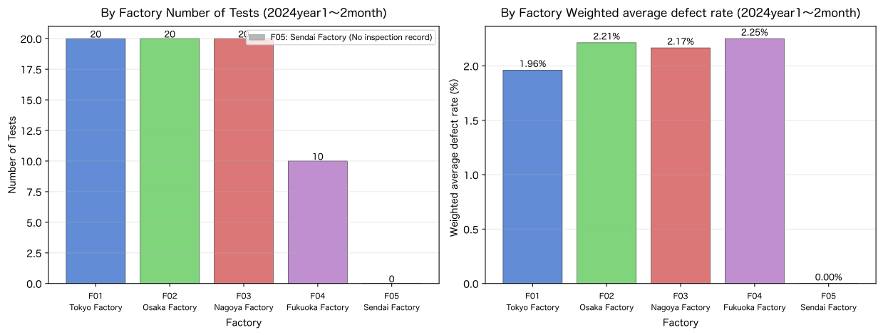

svg

Data overview graph display completed (SVG 1/2)

No.041: Join Tables with INNER JOIN

Meaning in Practice

INNER JOIN retrieves 2Common parts of the tables (data matching both). Main use cases in manufacturing:

Creating highly readable reports by attaching factory names and regions to inspection records
Combine parts master and performance to calculate loss amounts
Only achievement records with valid master codes are counted

Approach to Analysis and Modeling

\text{INNER JOIN}(A,\, B,\, \text{key}) = \{\,(a,\, b) \mid a \in A,\; b \in B,\; a.\text{key} = b.\text{key}\,\}

The binding key will be Rows that do not exist on one table are automatically excluded.. This differs from the traditional comma conjunction using WHERE clauses; the intent is clear.

-- Modern Writing Style (Recommended)
SELECT * FROM A INNER JOIN B ON A.key = B.key;
-- Traditional Writing Style (Not Recommended)
SELECT * FROM A, B WHERE A.key = B.key;

Check with Python

# No.041: INNER JOIN — Inspection Records × Factory Master

print('=== INNER JOIN: Factory information is attached to inspection records (first10Item)===')
q(conn, '''
SELECT i.id,
       i.inspection_date,
       i.factory_id,
       f.factory_name,
       f.region,
       i.line_code,
       i.production_qty,
       i.defect_qty
FROM   inspections i
INNER  JOIN factories f ON i.factory_id = f.factory_id
ORDER  BY i.id
LIMIT  10
''')

print()
print('=== INNER JOIN Subsequent full confirmation of the number of cases ===')
q(conn, '''
SELECT COUNT(*) AS inner_join_count
FROM   inspections i
INNER  JOIN factories f ON i.factory_id = f.factory_id
''')

=== INNER JOIN: Adds factory information to inspection records (Top 10 entries) ===
── SQL ─────────────────────────────────────────
  SELECT i.id,
         i.inspection_date,
         i.factory_id,
         f.factory_name,
         f.region,
         i.line_code,
         i.production_qty,
         i.defect_qty
  FROM   inspections i
  INNER  JOIN factories f ON i.factory_id = f.factory_id
  ORDER  BY i.id
  LIMIT  10
───────────────────────────────────────────────
shape: (10, 8)
┌─────┬───────────────┬────────────┬──────────────┬────────┬───────────┬──────────────┬────────────┐
│ id  ┆ inspection_da ┆ factory_id ┆ factory_name ┆ region ┆ line_code ┆ production_q ┆ defect_qty │
│ --- ┆ te            ┆ ---        ┆ ---          ┆ ---    ┆ ---       ┆ ty           ┆ ---        │
│ i64 ┆ ---           ┆ str        ┆ str          ┆ str    ┆ str       ┆ ---          ┆ i64        │
│     ┆ str           ┆            ┆              ┆        ┆           ┆ i64          ┆            │
╞═════╪═══════════════╪════════════╪══════════════╪════════╪═══════════╪══════════════╪════════════╡
│ 1   ┆ 2024-01-10    ┆ F01        ┆ Tokyo Factory     ┆ Kanto   ┆ LINE-A1   ┆ 471          ┆ 8          │
│ 2   ┆ 2024-01-10    ┆ F01        ┆ Tokyo Factory     ┆ Kanto   ┆ LINE-A1   ┆ 474          ┆ 10         │
│ 3   ┆ 2024-01-10    ┆ F01        ┆ Tokyo Factory     ┆ Kanto   ┆ LINE-A2   ┆ 296          ┆ 6          │
│ 4   ┆ 2024-01-10    ┆ F01        ┆ Tokyo Factory     ┆ Kanto   ┆ LINE-A2   ┆ 323          ┆ 7          │
│ 5   ┆ 2024-01-10    ┆ F02        ┆ Osaka Factory     ┆ Kansai   ┆ LINE-B1   ┆ 371          ┆ 8          │
│ 6   ┆ 2024-01-10    ┆ F02        ┆ Osaka Factory     ┆ Kansai   ┆ LINE-B1   ┆ 371          ┆ 7          │
│ 7   ┆ 2024-01-10    ┆ F02        ┆ Osaka Factory     ┆ Kansai   ┆ LINE-B2   ┆ 202          ┆ 4          │
│ 8   ┆ 2024-01-10    ┆ F02        ┆ Osaka Factory     ┆ Kansai   ┆ LINE-B2   ┆ 182          ┆ 5          │
│ 9   ┆ 2024-01-10    ┆ F03        ┆ Nagoya Factory   ┆ Central region   ┆ LINE-C1   ┆ 142          ┆ 4          │
│ 10  ┆ 2024-01-10    ┆ F03        ┆ Nagoya Factory   ┆ Central region   ┆ LINE-C1   ┆ 143          ┆ 3          │
└─────┴───────────────┴────────────┴──────────────┴────────┴───────────┴──────────────┴────────────┘
↳ Obtained in 10 lines

=== Checking the total number of cases after INNER JOIN ===
── SQL ─────────────────────────────────────────
  SELECT COUNT(*) AS inner_join_count
  FROM   inspections i
  INNER  JOIN factories f ON i.factory_id = f.factory_id
───────────────────────────────────────────────
shape: (1, 1)
┌──────────────────┐
│ inner_join_count │
│ ---              │
│ i64              │
╞══════════════════╡
│ 73               │
└──────────────────┘
↳ Obtain in 1 line

shape: (1, 1)

inner_join_count
i64
73

Reading the results

factory_name and region have been added to inspection records, greatly improving readability
The total number of INNER JOIN is 73records (equal to the total number of inspections). You can verify that valid factory_id exist in all test records
Three cases of fraud part_code = 'UNKNOWN-999' were not ruled out because factory_id were normal. Detect mismatches when coupling with the component master (No.045, No.050)

No.042: Join One Table Based on a LEFT JOIN

Meaning in Practice

LEFT JOIN Hold the entire row of the left table and complements NULL if there is no match in the right table. Main use cases in manufacturing:

View a list of all factories and visualize Factories without inspection records with NULL
View a list of all items and identify Uninspected Parts
“All-Checking Completeness” to comprehensively check all items present in the master

Approach to Analysis and Modeling

\text{LEFT JOIN}(A, B) \supseteq \text{INNER JOIN}(A, B)

The result of the LEFT JOIN always includes the result of the INNER JOIN. Rows that exist in the left table but do not match in the right table are added.

Situation	INNER JOIN	LEFT JOIN
Lines matching A and B	✅ exert effort	✅ exert effort
A line that exists only in A	❌ except	✅ Output (NULL on side B)
A line that exists only in B	❌ except	❌ except

Check with Python

# No.042: LEFT JOIN — Aggregates inspection performance based on all factories (F05 is displayed as 0 items)

print('=== LEFT JOIN: Number of inspections completed at all factories (F05 is NULL / 0 (It will be)===')
q(conn, '''
SELECT f.factory_id,
       f.factory_name,
       f.region,
       f.capacity,
       COUNT(i.id)                           AS inspection_count,
       COALESCE(SUM(i.production_qty), 0)    AS total_prod,
       COALESCE(SUM(i.defect_qty), 0)        AS total_defect
FROM   factories f
LEFT   JOIN inspections i ON f.factory_id = i.factory_id
GROUP  BY f.factory_id, f.factory_name, f.region, f.capacity
ORDER  BY inspection_count DESC
''')

=== LEFT JOIN: Number of inspections at all factories (F05 becomes NULL / 0) ===
── SQL ─────────────────────────────────────────
  SELECT f.factory_id,
         f.factory_name,
         f.region,
         f.capacity,
         COUNT(i.id)                           AS inspection_count,
         COALESCE(SUM(i.production_qty), 0)    AS total_prod,
         COALESCE(SUM(i.defect_qty), 0)        AS total_defect
  FROM   factories f
  LEFT   JOIN inspections i ON f.factory_id = i.factory_id
  GROUP  BY f.factory_id, f.factory_name, f.region, f.capacity
  ORDER  BY inspection_count DESC
───────────────────────────────────────────────
shape: (5, 7)
┌────────────┬──────────────┬────────┬──────────┬──────────────────┬────────────┬──────────────┐
│ factory_id ┆ factory_name ┆ region ┆ capacity ┆ inspection_count ┆ total_prod ┆ total_defect │
│ ---        ┆ ---          ┆ ---    ┆ ---      ┆ ---              ┆ ---        ┆ ---          │
│ str        ┆ str          ┆ str    ┆ i64      ┆ i64              ┆ i64        ┆ i64          │
╞════════════╪══════════════╪════════╪══════════╪══════════════════╪════════════╪══════════════╡
│ F01        ┆ Tokyo Factory     ┆ Kanto   ┆ 2000     ┆ 21               ┆ 8046       ┆ 157          │
│ F02        ┆ Osaka Factory     ┆ Kansai   ┆ 1800     ┆ 21               ┆ 6158       ┆ 140          │
│ F03        ┆ Nagoya Factory   ┆ Central region   ┆ 1600     ┆ 21               ┆ 4395       ┆ 101          │
│ F04        ┆ Fukuoka Factory     ┆ Kyushu   ┆ 1200     ┆ 10               ┆ 3466       ┆ 78           │
│ F05        ┆ Sendai Factory     ┆ Northeast   ┆ 1000     ┆ 0                ┆ 0          ┆ 0            │
└────────────┴──────────────┴────────┴──────────┴──────────────────┴────────────┴──────────────┘
↳ Obtained in 5 rows

shape: (5, 7)

factory_id	factory_name	region	capacity	inspection_count	total_prod	total_defect
str	str	str	i64	i64	i64	i64
”F01"	"Tokyo Factory"	"Kanto”	2000	21	8046	157
”F02"	"Osaka Factory"	"Kansai”	1800	21	6158	140
”F03"	"Nagoya Factory"	"Central region”	1600	21	4395	101
”F04"	"Fukuoka Factory"	"Kyushu”	1200	10	3466	78
”F05"	"Sendai Factory"	"Northeast”	1000	0	0	0

Reading the results

F05(Sendai Factory) is displayed as inspection_count = 0 and total_prod = 0. In INNER JOIN, the F05 line itself disappeared, but in LEFT JOIN, it resurfaces
By using COALESCE(SUM(...), 0), NULL is converted to 0. If the total value of F05 remains NULL, errors may occur in subsequent calculations
With the discovery of factories with no inspection records, we are now discussing whether it was before operations started or if there was a data linkage gap. It can be an opportunity to conduct research. This is a crucial confirmation that serves as the starting point for data quality management

No.043: Understanding the Concept of RIGHT JOIN

Meaning in Practice

RIGHT JOIN is the reverse version of LEFT JOIN, and it Hold the entire row of the right table. A RIGHT JOIN B is equivalent to B LEFT JOIN A.

In practice, LEFT JOIN (rearranging table order) is preferred over RIGHT JOIN. Reason: LEFT JOIN makes it intuitive and easy to understand what to use as a standard.

Approach to Analysis and Modeling

A \text{ RIGHT JOIN } B \equiv B \text{ LEFT JOIN } A

Either method yields the same results. Many teams also have coding policies that “always use LEFT JOIN.”

How to write	Holding side	excluded side
`A LEFT JOIN B`	All lines of A	B-only row
`A RIGHT JOIN B`	All lines of B	A line only
`A FULL OUTER JOIN B`	Both full lines	None (SQLite is not supported)

Check with Python

# No.043: RIGHT JOIN — Confirm the result is the same as the LEFT JOIN in No.042

print('=== RIGHT JOIN（inspections Left,factories (right)===')
df_right = q(conn, '''
SELECT f.factory_id,
       f.factory_name,
       COUNT(i.id) AS inspection_count
FROM   inspections i
RIGHT  JOIN factories f ON i.factory_id = f.factory_id
GROUP  BY f.factory_id, f.factory_name
ORDER  BY f.factory_id
''')

print()
print('=== equivalent LEFT JOIN(Swapping table order)===')
df_left = q(conn, '''
SELECT f.factory_id,
       f.factory_name,
       COUNT(i.id) AS inspection_count
FROM   factories f
LEFT   JOIN inspections i ON f.factory_id = i.factory_id
GROUP  BY f.factory_id, f.factory_name
ORDER  BY f.factory_id
''')

right_vals = sorted(df_right['inspection_count'].to_list())
left_vals  = sorted(df_left['inspection_count'].to_list())
print()
print(f'RIGHT JOIN Number of Results: {len(df_right)}')
print(f'LEFT  JOIN Number of Results: {len(df_left)}')
print(f'The two are equivalent.: {right_vals == left_vals}')

=== RIGHT JOIN (inspections on the left, factories on the right) ===
── SQL ─────────────────────────────────────────
  SELECT f.factory_id,
         f.factory_name,
         COUNT(i.id) AS inspection_count
  FROM   inspections i
  RIGHT  JOIN factories f ON i.factory_id = f.factory_id
  GROUP  BY f.factory_id, f.factory_name
  ORDER  BY f.factory_id
───────────────────────────────────────────────
shape: (5, 3)
┌────────────┬──────────────┬──────────────────┐
│ factory_id ┆ factory_name ┆ inspection_count │
│ ---        ┆ ---          ┆ ---              │
│ str        ┆ str          ┆ i64              │
╞════════════╪══════════════╪══════════════════╡
│ F01        ┆ Tokyo Factory     ┆ 21               │
│ F02        ┆ Osaka Factory     ┆ 21               │
│ F03        ┆ Nagoya Factory   ┆ 21               │
│ F04        ┆ Fukuoka Factory     ┆ 10               │
│ F05        ┆ Sendai Factory     ┆ 0                │
└────────────┴──────────────┴──────────────────┘
↳ Obtained in 5 rows

=== Equivalent LEFT JOIN (Rearranging Table Order) ===
── SQL ─────────────────────────────────────────
  SELECT f.factory_id,
         f.factory_name,
         COUNT(i.id) AS inspection_count
  FROM   factories f
  LEFT   JOIN inspections i ON f.factory_id = i.factory_id
  GROUP  BY f.factory_id, f.factory_name
  ORDER  BY f.factory_id
───────────────────────────────────────────────
shape: (5, 3)
┌────────────┬──────────────┬──────────────────┐
│ factory_id ┆ factory_name ┆ inspection_count │
│ ---        ┆ ---          ┆ ---              │
│ str        ┆ str          ┆ i64              │
╞════════════╪══════════════╪══════════════════╡
│ F01        ┆ Tokyo Factory     ┆ 21               │
│ F02        ┆ Osaka Factory     ┆ 21               │
│ F03        ┆ Nagoya Factory   ┆ 21               │
│ F04        ┆ Fukuoka Factory     ┆ 10               │
│ F05        ┆ Sendai Factory     ┆ 0                │
└────────────┴──────────────┴──────────────────┘
↳ Obtained in 5 rows

RIGHT JOIN Results: 5
LEFT JOIN Results: 5
Both are equivalent: True

Reading the results

You can confirm that the results of RIGHT JOIN and LEFT JOIN (rearranging the table order) are exactly the same
RIGHT JOIN has been supported since SQLite 3.39, In many settings, it is LEFT JOIN unified to maintain readability
FULL OUTER JOIN (holding all rows of both tables) is not supported in SQLite. If needed, you can approximate it with LEFT JOIN UNION ALL RIGHT JOIN

No.044: Combining Factory Master and Inspection Records

Meaning in Practice

Factory Master (factory name, region, capacity) and Test Record (number of productions and defects) By JOINing, you can automatically generate KPI summaries for regions and factories.

Examples of use in manufacturing:

Automation of Factory-Specific Monthly Production Reports for Management Meetings
Comparison of defect rates by region (Kanto / Kansai / Chubu / Kyushu)
Utilization rate analysis comparing capacity (capacity) and actual production numbers

Approach to Analysis and Modeling

When calculating the amount of defect loss, the cost gap (labor and equipment costs) by factory is factories You can handle this by extending the table.

\text{Uptime} = \frac{\text{Actual production numbers}}{\text{Factory capacity} \times \text{Number of days operated}}

Check with Python

# No.044: Factory Master × Inspection Records — Factory-Specific KPI Aggregation (Exclusion of Fraudulent Codes)

print('=== By Factory KPI Summary (INNER JOIN + Except for fraudulent codes)===')
q(conn, '''
SELECT f.factory_id,
       f.factory_name,
       f.region,
       f.capacity,
       COUNT(i.id)                                                    AS n_records,
       SUM(i.production_qty)                                          AS total_prod,
       SUM(i.defect_qty)                                              AS total_defect,
       ROUND(SUM(i.defect_qty) * 100.0 / SUM(i.production_qty), 2)  AS dr_pct,
       ROUND(SUM(i.production_qty) * 1.0 / f.capacity, 1)           AS prod_per_capacity
FROM   factories f
INNER  JOIN inspections i ON f.factory_id = i.factory_id
WHERE  i.part_code != 'UNKNOWN-999'
GROUP  BY f.factory_id, f.factory_name, f.region, f.capacity
ORDER  BY dr_pct DESC
''')

=== Factory-specific KPI Summary (INNER JOIN + Malicious Code Excluded) ===
── SQL ─────────────────────────────────────────
  SELECT f.factory_id,
         f.factory_name,
         f.region,
         f.capacity,
         COUNT(i.id)                                                    AS n_records,
         SUM(i.production_qty)                                          AS total_prod,
         SUM(i.defect_qty)                                              AS total_defect,
         ROUND(SUM(i.defect_qty) * 100.0 / SUM(i.production_qty), 2)  AS dr_pct,
         ROUND(SUM(i.production_qty) * 1.0 / f.capacity, 1)           AS prod_per_capacity
  FROM   factories f
  INNER  JOIN inspections i ON f.factory_id = i.factory_id
  WHERE  i.part_code != 'UNKNOWN-999'
  GROUP  BY f.factory_id, f.factory_name, f.region, f.capacity
  ORDER  BY dr_pct DESC
───────────────────────────────────────────────
shape: (4, 9)
┌────────────┬─────────────┬────────┬──────────┬───┬────────────┬────────────┬────────┬────────────┐
│ factory_id ┆ factory_nam ┆ region ┆ capacity ┆ … ┆ total_prod ┆ total_defe ┆ dr_pct ┆ prod_per_c │
│ ---        ┆ e           ┆ ---    ┆ ---      ┆   ┆ ---        ┆ ct         ┆ ---    ┆ apacity    │
│ str        ┆ ---         ┆ str    ┆ i64      ┆   ┆ i64        ┆ ---        ┆ f64    ┆ ---        │
│            ┆ str         ┆        ┆          ┆   ┆            ┆ i64        ┆        ┆ f64        │
╞════════════╪═════════════╪════════╪══════════╪═══╪════════════╪════════════╪════════╪════════════╡
│ F04        ┆ Fukuoka Factory    ┆ Kyushu   ┆ 1200     ┆ … ┆ 3466       ┆ 78         ┆ 2.25   ┆ 2.9        │
│ F02        ┆ Osaka Factory    ┆ Kansai   ┆ 1800     ┆ … ┆ 5783       ┆ 128        ┆ 2.21   ┆ 3.2        │
│ F03        ┆ Nagoya Factory  ┆ Central region   ┆ 1600     ┆ … ┆ 4247       ┆ 92         ┆ 2.17   ┆ 2.7        │
│ F01        ┆ Tokyo Factory    ┆ Kanto   ┆ 2000     ┆ … ┆ 7596       ┆ 149        ┆ 1.96   ┆ 3.8        │
└────────────┴─────────────┴────────┴──────────┴───┴────────────┴────────────┴────────┴────────────┘
↳ Obtained in 4 lines

shape: (4, 9)

factory_id	factory_name	region	capacity	n_records	total_prod	total_defect	dr_pct	prod_per_capacity
str	str	str	i64	i64	i64	i64	f64	f64
”F04"	"Fukuoka Factory"	"Kyushu”	1200	10	3466	78	2.25	2.9
”F02"	"Osaka Factory"	"Kansai”	1800	20	5783	128	2.21	3.2
”F03"	"Nagoya Factory"	"Central region”	1600	20	4247	92	2.17	2.7
”F01"	"Tokyo Factory"	"Kanto”	2000	20	7596	149	1.96	3.8

Reading the results

With region assigned, it becomes possible to compare Kanto vs Kansai vs Chubu vs Kyushu
prod_per_capacity (Production Quantity / Factory Capacity) is an estimate of capacity utilization. Higher lines have less room for increased production demands, leading to higher priority for capital investment
F05 (Sendai) will not appear in the results due to INNER JOIN. If you want to display all factories, use LEFT JOIN from No.042

No.045: Combining Part Master and Inspection Records

Meaning in Practice

By JOINING the Parts Master (part name, category, unit price) and Test Record, You can calculate the “defect loss amount” or “production value” for each part in a single query.

Examples of use in manufacturing:

Prioritizing improvement investments (starting with parts with large losses)
Comparison of KPIs by Category (Engine / Brakes / Electrical / Suspension)
ROI estimation based on unit price × number of defects

Approach to Analysis and Modeling

\text{Loss amount per part} = \sum_{i} \text{defect\_qty}_i \times \text{unit\_price}

Since the unit price of the component master is applied to each row after JOIN, SUM(i.defect_qty * p.unit_price) can be calculated correctly.

Check with Python

# No.045: Parts Master × Inspection Records — Loss Ranking by Part

print('=== By Component Production Value and Defect Loss (INNER JOIN）===')
q(conn, '''
SELECT p.part_code,
       p.part_name,
       p.category,
       p.unit_price,
       COUNT(i.id)                                                    AS n_records,
       SUM(i.production_qty)                                          AS total_prod,
       SUM(i.defect_qty)                                              AS total_defect,
       ROUND(SUM(i.defect_qty) * 100.0 / SUM(i.production_qty), 2)  AS dr_pct,
       SUM(i.production_qty * p.unit_price)                          AS production_value,
       SUM(i.defect_qty    * p.unit_price)                           AS defect_loss
FROM   parts p
INNER  JOIN inspections i ON p.part_code = i.part_code
GROUP  BY p.part_code, p.part_name, p.category, p.unit_price
ORDER  BY defect_loss DESC
''')

=== Production Value & Defect Loss by Component (INNER JOIN) ===
── SQL ─────────────────────────────────────────
  SELECT p.part_code,
         p.part_name,
         p.category,
         p.unit_price,
         COUNT(i.id)                                                    AS n_records,
         SUM(i.production_qty)                                          AS total_prod,
         SUM(i.defect_qty)                                              AS total_defect,
         ROUND(SUM(i.defect_qty) * 100.0 / SUM(i.production_qty), 2)  AS dr_pct,
         SUM(i.production_qty * p.unit_price)                          AS production_value,
         SUM(i.defect_qty    * p.unit_price)                           AS defect_loss
  FROM   parts p
  INNER  JOIN inspections i ON p.part_code = i.part_code
  GROUP  BY p.part_code, p.part_name, p.category, p.unit_price
  ORDER  BY defect_loss DESC
───────────────────────────────────────────────


shape: (5, 10)
┌───────────┬────────────┬────────────┬───────────┬───┬───────────┬────────┬───────────┬───────────┐
│ part_code ┆ part_name  ┆ category   ┆ unit_pric ┆ … ┆ total_def ┆ dr_pct ┆ productio ┆ defect_lo │
│ ---       ┆ ---        ┆ ---        ┆ e         ┆   ┆ ect       ┆ ---    ┆ n_value   ┆ ss        │
│ str       ┆ str        ┆ str        ┆ ---       ┆   ┆ ---       ┆ f64    ┆ ---       ┆ ---       │
│           ┆            ┆            ┆ i64       ┆   ┆ i64       ┆        ┆ i64       ┆ i64       │
╞═══════════╪════════════╪════════════╪═══════════╪═══╪═══════════╪════════╪═══════════╪═══════════╡
│ ENG-002   ┆ Cranksy ┆ Engine section ┆ 8500      ┆ … ┆ 78        ┆ 2.25   ┆ 29461000  ┆ 663000    │
│           ┆ Yaft     ┆ product         ┆           ┆   ┆           ┆        ┆           ┆           │
│ ELC-001   ┆ Alterne ┆ electrical components   ┆ 6800      ┆ … ┆ 59        ┆ 2.96   ┆ 13545600  ┆ 401200    │
│           ┆ ta         ┆            ┆           ┆   ┆           ┆        ┆           ┆           │
│ ENG-001   ┆ Piston ri ┆ Engine section ┆ 1200      ┆ … ┆ 159       ┆ 1.9    ┆ 10047600  ┆ 190800    │
│           ┆ Ng       ┆ product         ┆           ┆   ┆           ┆        ┆           ┆           │
│ BRK-001   ┆ brake pad ┆ Brake section ┆ 950       ┆ … ┆ 116       ┆ 1.99   ┆ 5547050   ┆ 110200    │
│           ┆ Dd       ┆ product         ┆           ┆   ┆           ┆        ┆           ┆           │
│ SUS-001   ┆ shock a ┆ Suspension ┆ 2800      ┆ … ┆ 35        ┆ 2.46   ┆ 3981600   ┆ 98000     │
│           ┆ busoba   ┆ Yon       ┆           ┆   ┆           ┆        ┆           ┆           │
└───────────┴────────────┴────────────┴───────────┴───┴───────────┴────────┴───────────┴───────────┘
↳ Obtained in 5 rows

shape: (5, 10)

part_code	part_name	category	unit_price	n_records	total_prod	total_defect	dr_pct	production_value	defect_loss
str	str	str	i64	i64	i64	i64	f64	i64	i64
”ENG-002"	"Crankshaft"	"Engine parts”	8500	10	3466	78	2.25	29461000	663000
”ELC-001"	"Alternator"	"electrical components”	6800	10	1992	59	2.96	13545600	401200
”ENG-001"	"piston ring"	"Engine parts”	1200	20	8373	159	1.9	10047600	190800
”BRK-001"	"brake pad"	"brake parts”	950	20	5839	116	1.99	5547050	110200
”SUS-001"	"shock absorber"	"suspension”	2800	10	1422	35	2.46	3981600	98000

Reading the results

defect_loss the top parts (defect loss amount) are the Top Priority Target for improvement investments. High-priced parts (ENG-002: ¥8,500 / ELC-001: ¥6,800) Even if the number of defects is small, the loss amount can be large
The three parts, BRK-002 / ELC-002 / SUS-002, do not have matching rows in the inspections, Not displayed. the results of INNER JOIN. (The left side is ‘parts’, so you can display it with LEFT JOIN)
If the “Defect Ranking” and “Loss Amount Ranking” differ, By prioritizing based on loss amounts, you can accurately assess Operational Impact

No.046: Joining Multiple Tables

Meaning in Practice

By 4Tables at once JOIN factory, line, parts, and inspection records, “Which factory, on which line, and which part has the highest defect rate?” You can grasp it with a single query.

Examples of use in manufacturing:

Generation of data for multi-axis KPI dashboards for management meetings
Cross-tabulation of factory × line × parts categories
Automatically assigning line names and capacity information to performance data

Approach to Analysis and Modeling

JOIN for multiple tables is written with the order of joins in mind.

FROM   inspections i
INNER  JOIN factories f ON i.factory_id = f.factory_id
INNER  JOIN lines l     ON i.line_code  = l.line_code
INNER  JOIN parts p     ON i.part_code  = p.part_code

The database engine optimizes the execution order, The join order prioritizes the query’s intent (the table you want to narrow down first).

Check with Python

# No.046: 4-Table INNER JOIN — Factory × Line × Parts KPI Aggregation

print('=== 4Table joining: Factory × Line × Parts Category Aggregate ===')
q(conn, '''
SELECT f.factory_name,
       f.region,
       l.line_name,
       p.part_name,
       p.category,
       COUNT(i.id)                                                    AS n_records,
       SUM(i.production_qty)                                          AS total_prod,
       SUM(i.defect_qty)                                              AS total_defect,
       ROUND(SUM(i.defect_qty) * 100.0 / SUM(i.production_qty), 2)  AS dr_pct
FROM   inspections i
INNER  JOIN factories f ON i.factory_id = f.factory_id
INNER  JOIN lines l     ON i.line_code  = l.line_code
INNER  JOIN parts p     ON i.part_code  = p.part_code
GROUP  BY f.factory_id, l.line_code, p.part_code
ORDER  BY f.factory_id, dr_pct DESC
''')

=== 4-Table Joining: Factory × Line × Part Category Aggregation ===
── SQL ─────────────────────────────────────────
  SELECT f.factory_name,
         f.region,
         l.line_name,
         p.part_name,
         p.category,
         COUNT(i.id)                                                    AS n_records,
         SUM(i.production_qty)                                          AS total_prod,
         SUM(i.defect_qty)                                              AS total_defect,
         ROUND(SUM(i.defect_qty) * 100.0 / SUM(i.production_qty), 2)  AS dr_pct
  FROM   inspections i
  INNER  JOIN factories f ON i.factory_id = f.factory_id
  INNER  JOIN lines l     ON i.line_code  = l.line_code
  INNER  JOIN parts p     ON i.part_code  = p.part_code
  GROUP  BY f.factory_id, l.line_code, p.part_code
  ORDER  BY f.factory_id, dr_pct DESC
───────────────────────────────────────────────
shape: (7, 9)
┌────────────┬────────┬────────────┬────────────┬───┬───────────┬────────────┬────────────┬────────┐
│ factory_na ┆ region ┆ line_name  ┆ part_name  ┆ … ┆ n_records ┆ total_prod ┆ total_defe ┆ dr_pct │
│ me         ┆ ---    ┆ ---        ┆ ---        ┆   ┆ ---       ┆ ---        ┆ ct         ┆ ---    │
│ ---        ┆ str    ┆ str        ┆ str        ┆   ┆ i64       ┆ i64        ┆ ---        ┆ f64    │
│ str        ┆        ┆            ┆            ┆   ┆           ┆            ┆ i64        ┆        │
╞════════════╪════════╪════════════╪════════════╪═══╪═══════════╪════════════╪════════════╪════════╡
│ Tokyo Factory   ┆ Kanto   ┆ Engine section ┆ Piston ri ┆ … ┆ 10        ┆ 4582       ┆ 90         ┆ 1.96   │
│            ┆        ┆ Product Line   ┆ Ng       ┆   ┆           ┆            ┆            ┆        │
│ Tokyo Factory   ┆ Kanto   ┆ Brake section ┆ brake pad ┆ … ┆ 10        ┆ 3014       ┆ 59         ┆ 1.96   │
│            ┆        ┆ Product Line   ┆ Dd       ┆   ┆           ┆            ┆            ┆        │
│ Osaka Factory   ┆ Kansai   ┆ Electrical Components ┆ Alterne ┆ … ┆ 10        ┆ 1992       ┆ 59         ┆ 2.96   │
│            ┆        ┆ Inn       ┆ ta         ┆   ┆           ┆            ┆            ┆        │
│ Osaka Factory   ┆ Kansai   ┆ Engine section ┆ Piston ri ┆ … ┆ 10        ┆ 3791       ┆ 69         ┆ 1.82   │
│            ┆        ┆ Product Line   ┆ Ng       ┆   ┆           ┆            ┆            ┆        │
│ Nagoya Factory ┆ Central region   ┆ Suspension ┆ shock a ┆ … ┆ 10        ┆ 1422       ┆ 35         ┆ 2.46   │
│            ┆        ┆ Jönlein ┆ busoba   ┆   ┆           ┆            ┆            ┆        │
│ Nagoya Factory ┆ Central region   ┆ Brake section ┆ brake pad ┆ … ┆ 10        ┆ 2825       ┆ 57         ┆ 2.02   │
│            ┆        ┆ Product Line   ┆ Dd       ┆   ┆           ┆            ┆            ┆        │
│ Fukuoka Factory   ┆ Kyushu   ┆ Engine section ┆ Cranksy ┆ … ┆ 10        ┆ 3466       ┆ 78         ┆ 2.25   │
│            ┆        ┆ Product Line   ┆ Yaft     ┆   ┆           ┆            ┆            ┆        │
└────────────┴────────┴────────────┴────────────┴───┴───────────┴────────────┴────────────┴────────┘
↳ Obtained in 7 rows

shape: (7, 9)

factory_name	region	line_name	part_name	category	n_records	total_prod	total_defect	dr_pct
str	str	str	str	str	i64	i64	i64	f64
”Tokyo Factory"	"Kanto"	"Engine parts line"	"piston ring"	"Engine parts”	10	4582	90	1.96
”Tokyo Factory"	"Kanto"	"Brake Parts Line"	"brake pad"	"brake parts”	10	3014	59	1.96
”Osaka Factory"	"Kansai"	"Electrical Components Line"	"Alternator"	"electrical components”	10	1992	59	2.96
”Osaka Factory"	"Kansai"	"Engine parts line"	"piston ring"	"Engine parts”	10	3791	69	1.82
”Nagoya Factory"	"Central region"	"Suspension line"	"shock absorber"	"suspension”	10	1422	35	2.46
”Nagoya Factory"	"Central region"	"Brake Parts Line"	"brake pad"	"brake parts”	10	2825	57	2.02
”Fukuoka Factory"	"Kyushu"	"Engine parts line"	"Crankshaft"	"Engine parts”	10	3466	78	2.25

Reading the results

Four tables were combined, and factory name / region / line name / part name / category was assigned A highly readable summary can be generated in a single query.
Even within the same factory, defect rates can vary depending on the production line. This reflects differences in process design, work standards, and equipment condition
Since n_records is uniform (each line × 5 days × 2 shifts = 10 cases), dr_pct comparison is being conducted under fair conditions.

No.047: Pay attention to duplicate binding keys

Meaning in Practice

If the same key is exist multiple in the target table, The number of rows after merging increases compared to expected (fan-out).

Typical examples in manufacturing:

If the quality standards table is operated as the ‘Standard Revision History,’ There are two lines in the same part code: “Standard Standard (2024Q1)” and “Strict Standard (2024Q2)”.
When you JOIN the part master to this quality standard table, you Increase in line count

Approach to Analysis and Modeling

quality_specs In the table, five components have two rows (before and after the reference revision).

parts Number of lines	After INNER JOIN,	Reasons for the increase
8 lines	11 lines	ENG-001/002, BRK-001, ELC-001 each fan-out on two lines

Number of lines after \text{JOIN} = \sum_{k \in \text{keys}} | A_k| \times | B_k|

Here, $|A_k|$ and $|B_k|$ are the number of times key $k$ appears at each table.

Check with Python

# No.047: Duplicate Combine Keys — Confirmed Increase in Line Count in parts × quality_specs

print('=== parts（8Item)× quality_specs（11Item) INNER JOIN ===')
q(conn, '''
SELECT p.part_code,
       p.part_name,
       p.unit_price,
       qs.spec_type,
       qs.max_dr_pct,
       qs.effective_from
FROM   parts p
INNER  JOIN quality_specs qs ON p.part_code = qs.part_code
ORDER  BY p.part_code, qs.effective_from
''')

print()
print('=== Which parts meet which standards (checking for duplicates)===')
q(conn, '''
SELECT p.part_code,
       p.part_name,
       COUNT(qs.spec_id) AS spec_count
FROM   parts p
LEFT   JOIN quality_specs qs ON p.part_code = qs.part_code
GROUP  BY p.part_code, p.part_name
ORDER  BY spec_count DESC, p.part_code
''')

=== INNER JOIN of parts (8 entries) × quality_specs (11 entries) ===
── SQL ─────────────────────────────────────────
  SELECT p.part_code,
         p.part_name,
         p.unit_price,
         qs.spec_type,
         qs.max_dr_pct,
         qs.effective_from
  FROM   parts p
  INNER  JOIN quality_specs qs ON p.part_code = qs.part_code
  ORDER  BY p.part_code, qs.effective_from
───────────────────────────────────────────────
shape: (11, 6)
┌───────────┬────────────────────┬────────────┬───────────┬────────────┬────────────────┐
│ part_code ┆ part_name          ┆ unit_price ┆ spec_type ┆ max_dr_pct ┆ effective_from │
│ ---       ┆ ---                ┆ ---        ┆ ---       ┆ ---        ┆ ---            │
│ str       ┆ str                ┆ i64        ┆ str       ┆ f64        ┆ str            │
╞═══════════╪════════════════════╪════════════╪═══════════╪════════════╪════════════════╡
│ BRK-001   ┆ brake pad     ┆ 950        ┆ standard standard  ┆ 2.5        ┆ 2024-01-01     │
│ BRK-001   ┆ brake pad     ┆ 950        ┆ Strict standards  ┆ 2.0        ┆ 2024-03-01     │
│ BRK-002   ┆ brake caliper ┆ 4200       ┆ standard standard  ┆ 3.0        ┆ 2024-01-01     │
│ ELC-001   ┆ Alternator       ┆ 6800       ┆ standard standard  ┆ 3.5        ┆ 2024-01-01     │
│ ELC-001   ┆ Alternator       ┆ 6800       ┆ Strict standards  ┆ 3.0        ┆ 2024-03-01     │
│ …         ┆ …                  ┆ …          ┆ …         ┆ …          ┆ …              │
│ ENG-001   ┆ piston ring     ┆ 1200       ┆ standard standard  ┆ 2.0        ┆ 2024-01-01     │
│ ENG-001   ┆ piston ring     ┆ 1200       ┆ Strict standards  ┆ 1.5        ┆ 2024-03-01     │
│ ENG-002   ┆ Crankshaft   ┆ 8500       ┆ standard standard  ┆ 1.8        ┆ 2024-01-01     │
│ ENG-002   ┆ Crankshaft   ┆ 8500       ┆ Strict standards  ┆ 1.2        ┆ 2024-03-01     │
│ SUS-001   ┆ shock absorber ┆ 2800       ┆ standard standard  ┆ 2.8        ┆ 2024-01-01     │
└───────────┴────────────────────┴────────────┴───────────┴────────────┴────────────────┘
↳ Obtained in 11 rows

=== Which parts meet which standards (Checking for duplicates)===
── SQL ─────────────────────────────────────────
  SELECT p.part_code,
         p.part_name,
         COUNT(qs.spec_id) AS spec_count
  FROM   parts p
  LEFT   JOIN quality_specs qs ON p.part_code = qs.part_code
  GROUP  BY p.part_code, p.part_name
  ORDER  BY spec_count DESC, p.part_code
───────────────────────────────────────────────
shape: (8, 3)
┌───────────┬────────────────────┬────────────┐
│ part_code ┆ part_name          ┆ spec_count │
│ ---       ┆ ---                ┆ ---        │
│ str       ┆ str                ┆ i64        │
╞═══════════╪════════════════════╪════════════╡
│ BRK-001   ┆ brake pad     ┆ 2          │
│ ELC-001   ┆ Alternator       ┆ 2          │
│ ENG-001   ┆ piston ring     ┆ 2          │
│ ENG-002   ┆ Crankshaft   ┆ 2          │
│ BRK-002   ┆ brake caliper ┆ 1          │
│ ELC-002   ┆ Starter motor     ┆ 1          │
│ SUS-001   ┆ shock absorber ┆ 1          │
│ SUS-002   ┆ coil spring   ┆ 0          │
└───────────┴────────────────────┴────────────┘
↳ Obtained in 8 lines

shape: (8, 3)

part_code	part_name	spec_count
str	str	i64
”BRK-001"	"brake pad”	2
”ELC-001"	"Alternator”	2
”ENG-001"	"piston ring”	2
”ENG-002"	"Crankshaft”	2
”BRK-002"	"brake caliper”	1
”ELC-002"	"Starter motor”	1
”SUS-001"	"shock absorber”	1
”SUS-002"	"coil spring”	0

Reading the results

If you INNER JOIN parts (8 items) and quality_specs (11 items), you get 11records. This is because parts for ENG-001, ENG-002, BRK-001, and ELC-001 each have two rows (standard and strict standards)
SUS-002 is excluded from INNER JOIN due to lack of quality_specs standards (line 1 → line 0).
Practical Measures: If you want to use only the latest standards, use WHERE effective_from = MAX(...) You need to narrow down quality_specs before subqueries or JOIN

No.048: Confirm an increase in the number of cases after merging

Meaning in Practice

After executing JOIN, Habit of checking if the number of cases meets expectations This is the foundation of data engineering.

Importance in Manufacturing:

If you calculate SUM without noticing the increase in row count in aggregate queries, a double counting occurs.
When monthly report values suddenly increase, it is often caused by duplicate JOIN keys.
Ensuring quality by asserting COUNT(*) in CI/CD pipelines

Approach to Analysis and Modeling

Steps to check the number of cases before and after JOIN:

Number of cases before merging: SELECT COUNT(*) FROM parts → 8
After INNER JOIN: SELECT COUNT(*) FROM parts INNER JOIN quality_specs ... → 11 cases (increase)
After LEFT JOIN: SELECT COUNT(*) FROM parts LEFT JOIN quality_specs ... → 12 records (including the NULL line in SUS-002)
Identifying duplicate keys: GROUP BY key HAVING COUNT(*) > 1

Check with Python

# No.048: Gradually Confirm the Increase in the Number of Cases After Joining

parts_n = conn.execute('SELECT COUNT(*) FROM parts').fetchone()[0]
qs_n    = conn.execute('SELECT COUNT(*) FROM quality_specs').fetchone()[0]
inner_n = conn.execute('''
    SELECT COUNT(*) FROM parts
    INNER JOIN quality_specs ON parts.part_code = quality_specs.part_code
''').fetchone()[0]
left_n  = conn.execute('''
    SELECT COUNT(*) FROM parts
    LEFT  JOIN quality_specs ON parts.part_code = quality_specs.part_code
''').fetchone()[0]

print('=== JOIN Comparison of the number of cases before and after ===')
print(f'  parts         : {parts_n} records')
print(f'  quality_specs : {qs_n} records')
print(f'  INNER JOIN After : {inner_n} records  ← parts More {inner_n - parts_n} Increase in cases (duplicate keys)')
print(f'  LEFT  JOIN After : {left_n} records  ← INNER More {left_n - inner_n} Increase in cases (NULL rows: SUS-002）')

# Identify parts with duplicate keys in quality_specs
print()
print('=== quality_specs Duplicate within part_code ===')
q(conn, '''
SELECT part_code, COUNT(*) AS spec_count
FROM   quality_specs
GROUP  BY part_code
HAVING COUNT(*) > 1
ORDER  BY spec_count DESC, part_code
''')

=== Comparison of Cases Before and After JOIN ===
  Parts: 8 items
  quality_specs: 11 items
  After INNER JOIN: 11 items, 3 more than ← parts (duplicate keys)
  After LEFT JOIN: 12 entries ← 1 more than INNER (NULL line: SUS-002)

=== Overlapping within quality_specs part_code ===
── SQL ─────────────────────────────────────────
  SELECT part_code, COUNT(*) AS spec_count
  FROM   quality_specs
  GROUP  BY part_code
  HAVING COUNT(*) > 1
  ORDER  BY spec_count DESC, part_code
───────────────────────────────────────────────
shape: (4, 2)
┌───────────┬────────────┐
│ part_code ┆ spec_count │
│ ---       ┆ ---        │
│ str       ┆ i64        │
╞═══════════╪════════════╡
│ BRK-001   ┆ 2          │
│ ELC-001   ┆ 2          │
│ ENG-001   ┆ 2          │
│ ENG-002   ┆ 2          │
└───────────┴────────────┘
↳ Obtained in 4 lines

shape: (4, 2)

part_code	spec_count
str	i64
”BRK-001”	2
”ELC-001”	2
”ENG-001”	2
”ENG-002”	2

Reading the results

INNER JOIN After that, the number of parts items increased from 8 to 11. quality_specs The cause is four components (ENG-001/002, BRK-001, ELC-001) that have duplicate keys
LEFT JOIN After that, one more case increased, bringing the total to 12. SUS-002 will be added as a NULL line
Countermeasures: After JOIN, check the number of COUNT(*) and if there is any unintended increase, GROUP BY ... HAVING COUNT(*) > 1 Identify duplicate keys
Make it a habit to always check the number of entries before running aggregated queries (SUM / AVG)

No.049: Extracting Parts Without Inspection Records

Meaning in Practice

LEFT JOIN + WHERE IS NULL Patterns “Detecting what doesn’t exist” It is one of the most powerful SQL techniques.

Examples of use in manufacturing:

Although it is registered in the parts master, this fiscal year the parts are produced at zero (discontinued?) Missed the proper planning?)
Parts not registered with quality standards (risk management gaps)
On days when the performance hasn’t arrived from a line that should be operating (sensor abnormality?) Data integration error?)

Approach to Analysis and Modeling

\text{Uninspected parts} = \text{parts} - \text{INNER JOIN}(\text{parts},\, \text{inspections})

SELECT p.*
FROM   parts p
LEFT   JOIN inspections i ON p.part_code = i.part_code
WHERE  i.id IS NULL   -- ← Only rows with no match in the right table

WHERE i.id IS NULL extracts “NULL lines in LEFT JOIN = unrecorded parts.”

Check with Python

# No.049: Extracting parts without inspection experience using LEFT JOIN + WHERE IS NULL

# (1) Number of inspections for all items (LEFT JOIN + GROUP BY)
print('=== ① Number of inspections for all products (LEFT JOIN Zero parts are also displayed.)===')
df_parts_join = q(conn, '''
SELECT p.part_code,
       p.part_name,
       p.category,
       p.unit_price,
       COUNT(i.id) AS inspection_count
FROM   parts p
LEFT   JOIN inspections i ON p.part_code = i.part_code
GROUP  BY p.part_code, p.part_name, p.category, p.unit_price
ORDER  BY p.part_code
''')

print()
print('=== ② Only parts without inspection records (WHERE i.id IS NULL）===')
q(conn, '''
SELECT p.part_code,
       p.part_name,
       p.category,
       p.unit_price,
       p.supplier_code
FROM   parts p
LEFT   JOIN inspections i ON p.part_code = i.part_code
WHERE  i.id IS NULL
ORDER  BY p.part_code
''')

=== (1) Number of inspections for all products (LEFT JOIN also shows zero parts) ===
── SQL ─────────────────────────────────────────
  SELECT p.part_code,
         p.part_name,
         p.category,
         p.unit_price,
         COUNT(i.id) AS inspection_count
  FROM   parts p
  LEFT   JOIN inspections i ON p.part_code = i.part_code
  GROUP  BY p.part_code, p.part_name, p.category, p.unit_price
  ORDER  BY p.part_code
───────────────────────────────────────────────
shape: (8, 5)
┌───────────┬────────────────────┬────────────────┬────────────┬──────────────────┐
│ part_code ┆ part_name          ┆ category       ┆ unit_price ┆ inspection_count │
│ ---       ┆ ---                ┆ ---            ┆ ---        ┆ ---              │
│ str       ┆ str                ┆ str            ┆ i64        ┆ i64              │
╞═══════════╪════════════════════╪════════════════╪════════════╪══════════════════╡
│ BRK-001   ┆ brake pad     ┆ brake parts   ┆ 950        ┆ 20               │
│ BRK-002   ┆ brake caliper ┆ brake parts   ┆ 4200       ┆ 0                │
│ ELC-001   ┆ Alternator       ┆ electrical components       ┆ 6800       ┆ 10               │
│ ELC-002   ┆ Starter motor     ┆ electrical components       ┆ 3500       ┆ 0                │
│ ENG-001   ┆ piston ring     ┆ Engine parts   ┆ 1200       ┆ 20               │
│ ENG-002   ┆ Crankshaft   ┆ Engine parts   ┆ 8500       ┆ 10               │
│ SUS-001   ┆ shock absorber ┆ suspension ┆ 2800       ┆ 10               │
│ SUS-002   ┆ coil spring   ┆ suspension ┆ 1800       ┆ 0                │
└───────────┴────────────────────┴────────────────┴────────────┴──────────────────┘
↳ Obtained in 8 lines

=== (2) Only parts without inspection experience (WHERE i.id IS NULL) ===
── SQL ─────────────────────────────────────────
  SELECT p.part_code,
         p.part_name,
         p.category,
         p.unit_price,
         p.supplier_code
  FROM   parts p
  LEFT   JOIN inspections i ON p.part_code = i.part_code
  WHERE  i.id IS NULL
  ORDER  BY p.part_code
───────────────────────────────────────────────
shape: (3, 5)
┌───────────┬────────────────────┬────────────────┬────────────┬───────────────┐
│ part_code ┆ part_name          ┆ category       ┆ unit_price ┆ supplier_code │
│ ---       ┆ ---                ┆ ---            ┆ ---        ┆ ---           │
│ str       ┆ str                ┆ str            ┆ i64        ┆ str           │
╞═══════════╪════════════════════╪════════════════╪════════════╪═══════════════╡
│ BRK-002   ┆ brake caliper ┆ brake parts   ┆ 4200       ┆ SUP-02        │
│ ELC-002   ┆ Starter motor     ┆ electrical components       ┆ 3500       ┆ SUP-03        │
│ SUS-002   ┆ coil spring   ┆ suspension ┆ 1800       ┆ SUP-04        │
└───────────┴────────────────────┴────────────────┴────────────┴───────────────┘
↳ Retrieved in 3 lines

shape: (3, 5)

part_code	part_name	category	unit_price	supplier_code
str	str	str	i64	str
”BRK-002"	"brake caliper"	"brake parts”	4200	”SUP-02"
"ELC-002"	"Starter motor"	"electrical components”	3500	”SUP-03"
"SUS-002"	"coil spring"	"suspension”	1800	”SUP-04”

# No.049 Visualization: Number of Inspections by Part (Highlight Uninspected Parts in Red)
rows_p  = df_parts_join.to_dicts()
p_codes = [r['part_code'] for r in rows_p]
counts  = [r['inspection_count'] for r in rows_p]
bar_col = ['#D65F5F' if c == 0 else '#4878CF' for c in counts]

fig, ax = plt.subplots(figsize=(10, 5))
bars = ax.bar(range(len(p_codes)), counts, color=bar_col, alpha=0.85,
              edgecolor='black', linewidth=0.4)
for bar, v in zip(bars, counts):
    ax.text(bar.get_x() + bar.get_width() / 2, bar.get_height() + 0.3,
            str(v), ha='center', va='bottom', fontsize=9)
ax.set_xticks(range(len(p_codes)))
ax.set_xticklabels(p_codes, rotation=30, ha='right', fontsize=9)
ax.set_title('By Component Number of Tests (LEFT JOINCovers all items here)', fontsize=12, pad=10)
ax.set_xlabel('Part code', fontsize=10)
ax.set_ylabel('Number of Tests', fontsize=10)
ax.grid(axis='y', alpha=0.3)
legend_h = [
    Patch(color='#4878CF', alpha=0.85, label='Inspection track record'),
    Patch(color='#D65F5F', alpha=0.85, label='No inspection record (please confirm)'),
]
ax.legend(handles=legend_h, fontsize=9, loc='upper right')
plt.tight_layout()
plt.show()
print('Completion of Display of Inspection Count Graph by Part (SVG 2/2）')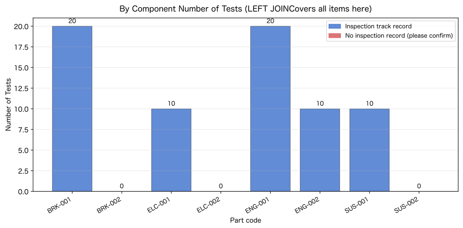

svg

Completion of graph display of inspection counts by part (SVG 2/2)

Reading the results

BRK-002 / ELC-002 / SUS-002 three parts will appear as zero inspection counts (red bar). Just by looking at the graph, you can instantly grasp the list of parts not inspected this fiscal year
These parts may not be allocated to this season’s lineup. This triggers the site to confirm whether production has been discontinued, is the setup being changed, or if there is a data linkage missing.
WHERE i.id IS NULL (NOT EXISTS pattern) can be used with SQLite, PostgreSQL, and MySQL. NOT IN (SELECT ...) also yields the same results, but since including NULL changes the behavior, LEFT JOIN + IS NULL is safer

No.050: Detecting inspection records missing in the component master

Meaning in Practice

This is the reverse pattern of No.049. This time “There is no master code to reference for the achievement data.” = Detects Isolated (Orphant) Records.

Examples of use in manufacturing:

Manual input errors or inspection records registered with old codes (such as UNKNOWN-999)
Achievement data remaining after master deletion (lack of deletion protection)
Unknown code slipped in due to data integration errors from external systems

Approach to Analysis and Modeling

\text{isolated record} = \text{inspections} - \text{INNER JOIN}(\text{inspections},\, \text{parts})

SELECT i.*
FROM   inspections i
LEFT   JOIN parts p ON i.part_code = p.part_code
WHERE  p.part_code IS NULL   -- ← parts There was no agreement = fraudulent code

It’s the same LEFT JOIN + WHERE IS NULL pattern as No.049, Pay attention to JOINThe direction (which is the reference) is reversed. things.

Check with Python

# No.050: Detection of Inspection Records (Fraudulent part_code) Not Present in the Component Master

print('=== fraud part_code detection (LEFT JOIN + WHERE p.part_code IS NULL）===')
q(conn, '''
SELECT i.id,
       i.inspection_date,
       i.factory_id,
       i.line_code,
       i.part_code          AS orphaned_part_code,
       i.shift,
       i.production_qty,
       i.defect_qty,
       p.part_name          AS part_name_check
FROM   inspections i
LEFT   JOIN parts p ON i.part_code = p.part_code
WHERE  p.part_code IS NULL
ORDER  BY i.id
''')

print()
print('=== Aggregation of fraudulent codes (which factory or line they came from)===')
q(conn, '''
SELECT i.factory_id, i.line_code,
       COUNT(*) AS orphaned_count,
       i.part_code AS orphaned_code
FROM   inspections i
LEFT   JOIN parts p ON i.part_code = p.part_code
WHERE  p.part_code IS NULL
GROUP  BY i.factory_id, i.line_code, i.part_code
ORDER  BY orphaned_count DESC
''')

=== Detection of Fraud part_code (LEFT JOIN + WHERE p.part_code IS NULL)===
── SQL ─────────────────────────────────────────
  SELECT i.id,
         i.inspection_date,
         i.factory_id,
         i.line_code,
         i.part_code          AS orphaned_part_code,
         i.shift,
         i.production_qty,
         i.defect_qty,
         p.part_name          AS part_name_check
  FROM   inspections i
  LEFT   JOIN parts p ON i.part_code = p.part_code
  WHERE  p.part_code IS NULL
  ORDER  BY i.id
───────────────────────────────────────────────
shape: (3, 9)
┌─────┬──────────────┬────────────┬───────────┬───┬───────┬─────────────┬────────────┬─────────────┐
│ id  ┆ inspection_d ┆ factory_id ┆ line_code ┆ … ┆ shift ┆ production_ ┆ defect_qty ┆ part_name_c │
│ --- ┆ ate          ┆ ---        ┆ ---       ┆   ┆ ---   ┆ qty         ┆ ---        ┆ heck        │
│ i64 ┆ ---          ┆ str        ┆ str       ┆   ┆ str   ┆ ---         ┆ i64        ┆ ---         │
│     ┆ str          ┆            ┆           ┆   ┆       ┆ i64         ┆            ┆ null        │
╞═════╪══════════════╪════════════╪═══════════╪═══╪═══════╪═════════════╪════════════╪═════════════╡
│ 71  ┆ 2024-01-15   ┆ F01        ┆ LINE-A1   ┆ … ┆ early shift  ┆ 450         ┆ 8          ┆ null        │
│ 72  ┆ 2024-01-22   ┆ F02        ┆ LINE-B1   ┆ … ┆ late shift  ┆ 375         ┆ 12         ┆ null        │
│ 73  ┆ 2024-02-10   ┆ F03        ┆ LINE-C1   ┆ … ┆ early shift  ┆ 148         ┆ 9          ┆ null        │
└─────┴──────────────┴────────────┴───────────┴───┴───────┴─────────────┴────────────┴─────────────┘
↳ Retrieved in 3 lines

=== Aggregation of Malicious Code (Which Factory or Line Came From)===
── SQL ─────────────────────────────────────────
  SELECT i.factory_id, i.line_code,
         COUNT(*) AS orphaned_count,
         i.part_code AS orphaned_code
  FROM   inspections i
  LEFT   JOIN parts p ON i.part_code = p.part_code
  WHERE  p.part_code IS NULL
  GROUP  BY i.factory_id, i.line_code, i.part_code
  ORDER  BY orphaned_count DESC
───────────────────────────────────────────────
shape: (3, 4)
┌────────────┬───────────┬────────────────┬───────────────┐
│ factory_id ┆ line_code ┆ orphaned_count ┆ orphaned_code │
│ ---        ┆ ---       ┆ ---            ┆ ---           │
│ str        ┆ str       ┆ i64            ┆ str           │
╞════════════╪═══════════╪════════════════╪═══════════════╡
│ F01        ┆ LINE-A1   ┆ 1              ┆ UNKNOWN-999   │
│ F02        ┆ LINE-B1   ┆ 1              ┆ UNKNOWN-999   │
│ F03        ┆ LINE-C1   ┆ 1              ┆ UNKNOWN-999   │
└────────────┴───────────┴────────────────┴───────────────┘
↳ Retrieved in 3 lines

shape: (3, 4)

factory_id	line_code	orphaned_count	orphaned_code
str	str	i64	str
”F01"	"LINE-A1”	1	”UNKNOWN-999"
"F02"	"LINE-B1”	1	”UNKNOWN-999"
"F03"	"LINE-C1”	1	”UNKNOWN-999”

Reading the results

Three cases of part_code = 'UNKNOWN-999' were detected. part_name_check is NULL. These are records with invalid codes that do not exist in the parts master
The source of the fraudulent code spans three factories: F01, F02, and F03. Higher likelihood of Data Integration Bug than manual input errors (occurring dispersed rather than from specific lines)
Response Procedure:
1. orphaned_count Contact data managers at factories and lines with high levels of
2. Identify the correct part_code and fix it with UPDATE or DELETE
3. Adding foreign key constraints (FOREIGN KEY) to prevent recurrence
LEFT JOIN + WHERE IS NULL Pattern as a practical Data Quality Check Query It is effective when incorporated into regular execution (cron / Airflow)

Practical Implications Seen Through Target Exercise

Through JOIN taught in No.041–050, the following manufacturing practical challenges can be solved using SQL.

Practical Issues	SQL Patterns
Factory name and region added to the track record	`INNER JOIN factories`
Unit price × Calculate loss amount based on number of defects	`INNER JOIN parts` + `SUM(defect * price)`
Covering all factories to identify zero-number factories	`LEFT JOIN factories ... COALESCE(...)`
Cross-table KPIs of 3 or more tables	`JOIN factories JOIN lines JOIN parts`
Prevention of miscalculations due to overlapping quality standards	Check `COUNT(*)` before and after JOIN
Identification of uninspected parts and unoperated lines	`LEFT JOIN ... WHERE IS NULL`
Detecting and remediating malicious code	`LEFT JOIN parts ... WHERE p.part_code IS NULL`

With the migration to VLOOKUP → SQL JOIN, monthly matchmaking can be reduced to 1query × a few seconds.

What is necessary for practical implementation

1. Establishment of foreign key constraints

In SQLite, foreign key constraints are disabled unless you run PRAGMA foreign_keys = ON;. In the production database (PostgreSQL / MySQL), set the FOREIGN KEY, DB Prevention at the level for the mixing of fraudulent codes.

2. Index Settings

The JOIN binding keys (factory_id, part_code, line_code) Setting an index speeds up JOIN on large volumes of data. CREATE INDEX idx_insp_part ON inspections(part_code);

3. Regular execution of LEFT JOIN + WHERE IS NULL

Incorporate data quality check queries (No.049, No.050) into the regular job, We will create a system that immediately sends alerts when fraudulent code or uninspected parts occur.

4. Assertions of the number of cases after JOIN combination

In ETL pipelines or monthly aggregation batches, you can add assertions using COUNT(*), We recommend designing a system that suspends processing or issues alerts when the expected number of cases is exceeded.

Conclusion

In this chapter, we used SQL JOIN to analyze multiple tables in the manufacturing performance database.

exercise	Main SQL	Key Points for Use in Manufacturing
No.041	`INNER JOIN`	Basic Combination with Factory Name and Unit Price Added to Performance
No.042	`LEFT JOIN`	Identifying factories with zero inspection records based on a whole-factory standard
No.043	`RIGHT JOIN`	Understanding the Equivalence with LEFT JOIN
No.044	`JOIN factories`	KPI (Defect Rate/Occupancy Rate) Aggregation by Factory
No.045	`JOIN parts`	Loss Ranking by Part
No.046	`JOIN × 3 chain`	Cross-section analysis of factory + line + parts + inspection records
No.047	Identifying duplicate keys	Increase in the number of rows due to duplicate quality standards tables
No.048	Number of Assertions	Quality assurance through `COUNT(*)` before and after JOIN
No.049	`LEFT JOIN + WHERE IS NULL`	Automatic identification of uninspected parts
No.050	`LEFT JOIN + WHERE IS NULL`	Automatic detection of fraudulent code

In the next chapter (Chapter 6: Subqueries and CTE), Learn how to build even more complex analytical queries in combination with JOIN.

Consultations for Corporations

Please feel free to consult us about data analysis, SQL education, and DX promotion in manufacturing using the information below.

📩 Contact Us: surikobo.co.jp/contact Please feel free to consult us first.

Perform cross-analysis of factory, parts, and inspection records using SQL JOINs

Perform cross-analysis of factory, parts, and inspection records using SQL JOINs

SQL 100 Exercises Chapter 5 (No.041–No.050): Table Join with JOIN

Introduction: Practical Challenges in Manufacturing Covered in This Article

Common situations on site

Why is this issue so difficult to judge?

1. Distinguishing Between INNER JOIN and LEFT JOIN

2. Increase in line count due to duplicate combination keys

3. Use IS NULL to determine NULL

4. Verification of Number of Cases Before and After Joining

Overview of Exercise covered this time

Preparing the Python environment

Creation of Fictional Data

No.041: Join Tables with INNER JOIN

Meaning in Practice

Approach to Analysis and Modeling

Check with Python

Reading the results

No.042: Join One Table Based on a LEFT JOIN

Meaning in Practice

Approach to Analysis and Modeling

Check with Python

Reading the results

No.043: Understanding the Concept of RIGHT JOIN

Meaning in Practice

Approach to Analysis and Modeling

Check with Python

Reading the results

No.044: Combining Factory Master and Inspection Records

Meaning in Practice

Approach to Analysis and Modeling

Check with Python

Reading the results

No.045: Combining Part Master and Inspection Records

Meaning in Practice

Approach to Analysis and Modeling

Check with Python

Reading the results

No.046: Joining Multiple Tables

Meaning in Practice

Approach to Analysis and Modeling

Check with Python

Reading the results

No.047: Pay attention to duplicate binding keys

Meaning in Practice

Approach to Analysis and Modeling

Check with Python

Reading the results

No.048: Confirm an increase in the number of cases after merging

Meaning in Practice

Approach to Analysis and Modeling

Check with Python

Reading the results

No.049: Extracting Parts Without Inspection Records

Meaning in Practice

Approach to Analysis and Modeling

Check with Python

Reading the results

No.050: Detecting inspection records missing in the component master

Meaning in Practice

Approach to Analysis and Modeling

Check with Python

Reading the results

Practical Implications Seen Through Target Exercise

What is necessary for practical implementation

1. Establishment of foreign key constraints

2. Index Settings

3. Regular execution of LEFT JOIN + WHERE IS NULL

4. Assertions of the number of cases after JOIN combination

Conclusion

Consultations for Corporations

Related Posts

Integrating data quality management, SQL design, and BI integration into production line operations

Deepening manufacturing decision-making with SQL application analysis techniques

Automate order KPIs, customer analysis, and inventory risk assessment using SQL

Analyze monthly trends on manufacturing lines from multiple perspectives using SQL window functions

Automating abnormality detection and KPI aggregation on production lines with subqueries and CTE

3. Use `IS NULL` to determine NULL