
100本ノック / 機械学習 / 実務機械学習100本ノック
製造業の機械学習モデル評価入門|交差検証・過学習・評価指標をPythonで実践
不良流出を防ぎながら検査負荷を抑える:製造業のモデル評価と検証 10本ノック
製造条件から「重点検査すべきロット」を予測する架空の品質管理ケースを通して、No.041〜No.050のモデル評価と検証を実践します。精度が高いというだけでモデルを採用せず、将来データへの再現性、探索の妥当性、過学習、説明可能性、そして不良流出と追加検査のコストまでを一貫して確認します。
本記事で利用するデータ、工場名、設備名、費用はすべて架空です。外部データは使用しません。
[!NOTE] 本資料は、数理工房 (もしくは代表である和山個人) が過去に企業研修において使用した notebook を企業様の許可を得て再構成・編集のうえ公開しています。
掲載データはすべて架空のものであり、実在する企業・工場・数値とは一切関係ありません。
はじめに:この記事で扱う製造業の実務課題
架空の精密部品工場では、全ロットを同じ強度で検査すると検査工程がボトルネックになります。そこで、加工時の温度、圧力、振動、設備負荷などから不良リスクを予測し、高リスクのロットだけを重点検査する仕組みを検討します。
意思決定の中心は「どのアルゴリズムが最も高精度か」ではありません。未見の将来ロットでも性能が維持されるか、不良を見逃さないか、追加検査が現場の処理能力に収まるか、という運用上の問いです。
現場でよくある状況
- 開発時の正解率は高かったが、翌月のロットでは性能が落ちる
- 同じデータで何度もモデルを選び、テストデータに事実上合わせ込んでしまう
- 不良が少ないため、すべて良品と判定しても正解率が高く見える
- 見逃しと過剰検査の損失が異なるのに、評価指標が正解率だけになっている
なぜこの問題は判断が難しいのか
評価値はデータの切り方、時系列性、クラス比率、探索範囲によって変わります。また、統計的に良いモデルと現場で採用すべきモデルは一致しないことがあります。製造条件は設備摩耗や季節で変化するため、ランダム分割だけでは将来性能を楽観視するおそれもあります。
今回扱うノックの全体像
| No. | テーマ | 実務上の問い |
|---|---|---|
| 041 | ホールドアウト検証 | 未使用データで性能を測れているか |
| 042 | 交差検証 | 分割偶然性を考慮しているか |
| 043 | TimeSeriesSplit | 過去から未来を予測する検証か |
| 044 | GridSearchCV | 候補を漏れなく比較できるか |
| 045 | RandomizedSearchCV | 探索予算を効率配分できるか |
| 046 | 過学習 | 学習データだけに適合していないか |
| 047 | 学習曲線 | データ追加が効くのか |
| 048 | 特徴量重要度 | 予測を動かす条件は何か |
| 049 | 複数モデル比較 | 精度・安定性・説明性を比較したか |
| 050 | 実務指標 | 見逃しと検査負荷を金額で比べたか |
Python 環境の準備
乱数シードを固定し、同じ結果を再現できるようにします。前処理は Pipeline に含め、検証データの情報が学習側へ混入しない構成にします。グラフは matplotlib のみを使用します。
import sys
import warnings
import numpy as np
import pandas as pd
import matplotlib
import matplotlib.pyplot as plt
import sklearn

from sklearn.base import clone
from sklearn.compose import ColumnTransformer
from sklearn.preprocessing import StandardScaler
from sklearn.pipeline import Pipeline
from sklearn.model_selection import (
    train_test_split, StratifiedKFold, TimeSeriesSplit, cross_validate,
    GridSearchCV, RandomizedSearchCV, learning_curve
)
from sklearn.metrics import (
    accuracy_score, recall_score, precision_score, f1_score, roc_auc_score,
    confusion_matrix, make_scorer
)
from sklearn.linear_model import LogisticRegression
from sklearn.tree import DecisionTreeClassifier
from sklearn.ensemble import RandomForestClassifier, GradientBoostingClassifier

warnings.filterwarnings("ignore", message="Glyph .* missing from font")
SEED = 42
np.random.seed(SEED)
plt.rcParams["figure.figsize"] = (8, 4.5)

print("Python      :", sys.version.split()[0])
print("numpy       :", np.__version__)
print("pandas      :", pd.__version__)
print("matplotlib  :", matplotlib.__version__)
print("scikit-learn:", sklearn.__version__)
Python : 3.13.1
numpy : 2.5.1
pandas : 3.0.3
matplotlib : 3.11.0
scikit-learn: 1.9.0架空データの作成
900日分の製造ロットを生成します。後半ほど設備摩耗が進み、夏季には温度が上がる設定です。不良確率は温度・振動・圧力偏差・設備負荷・材料硬度・摩耗の非線形な組み合わせで決まります。is_defect=1 が重点検査で捉えたい不良ロットです。
rng = np.random.default_rng(SEED)
n = 900
date = pd.date_range("2023-01-01", periods=n, freq="D")
t = np.arange(n)
temperature = 68 + 7 * np.sin(2 * np.pi * t / 365) + 0.006 * t + rng.normal(0, 2.2, n)
pressure = 100 + rng.normal(0, 4.5, n) + 0.8 * np.sin(2 * np.pi * t / 30)
vibration = np.clip(1.6 + 0.0012 * t + rng.gamma(1.8, 0.28, n), 0, None)
machine_load = np.clip(rng.normal(72, 11, n) + 5 * np.sin(2 * np.pi * t / 7), 35, 100)
material_hardness = rng.normal(61, 3.2, n)
maintenance_days = np.mod(t, 120)

logit = (-4.8 + 0.10 * (temperature - 70) + 0.60 * (vibration - 2)
         + 0.035 * np.abs(pressure - 100) + 0.028 * (machine_load - 70)
         - 0.055 * (material_hardness - 60) + 0.010 * maintenance_days
         + 0.8 * ((temperature > 75) & (machine_load > 80)))
probability = 1 / (1 + np.exp(-logit))
is_defect = rng.binomial(1, probability)

df = pd.DataFrame({
    "date": date, "temperature": temperature, "pressure": pressure,
    "vibration": vibration, "machine_load": machine_load,
    "material_hardness": material_hardness,
    "maintenance_days": maintenance_days, "is_defect": is_defect
})
features = ["temperature", "pressure", "vibration", "machine_load",
            "material_hardness", "maintenance_days"]
X, y = df[features], df["is_defect"]

display(df.head().round(2))
print(f"ロット数: {len(df):,}")
print(f"不良ロット数: {y.sum():,}(不良率 {y.mean():.1%})")
/var/folders/3y/fmw40k0x78xblvb3gkcyvy1h0000gn/T/ipykernel_51844/3118308666.py:29: UserWarning: obj.round has no effect with datetime, timedelta, or period dtypes. Use obj.dt.round(...) instead.
display(df.head().round(2))| date | temperature | pressure | vibration | machine_load | material_hardness | maintenance_days | is_defect | |
|---|---|---|---|---|---|---|---|---|
| 0 | 2023-01-01 | 68.67 | 101.75 | 2.00 | 61.81 | 61.60 | 0 | 0 |
| 1 | 2023-01-02 | 65.84 | 100.63 | 1.92 | 89.41 | 58.75 | 1 | 0 |
| 2 | 2023-01-03 | 69.90 | 99.66 | 2.05 | 83.81 | 65.58 | 2 | 0 |
| 3 | 2023-01-04 | 70.45 | 107.62 | 2.20 | 82.17 | 63.91 | 3 | 0 |
| 4 | 2023-01-05 | 64.21 | 97.79 | 2.03 | 82.93 | 61.93 | 4 | 0 |
ロット数: 900
不良ロット数: 38(不良率 4.2%)
時系列の変化とクラス不均衡を最初に確認します。月次不良率は母数が小さいため振れますが、後半で条件が厳しくなる設計を読み取れます。
monthly = df.set_index("date")["is_defect"].resample("MS").agg(["mean", "count"])
fig, ax = plt.subplots()
ax.plot(monthly.index, monthly["mean"], marker="o", linewidth=1.5)
ax.set_title("Monthly defect rate (synthetic data)")
ax.set_xlabel("Month")
ax.set_ylabel("Defect rate")
ax.grid(True, alpha=0.3)
fig.tight_layout()
plt.show()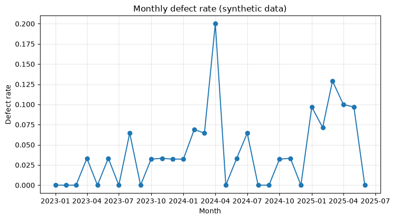
No.041:ホールドアウト検証を行う
実務での意味
モデル作成に使わないテストデータを確保し、導入前の疑似本番として評価します。品質用途では不良率を保つため、目的変数で層化して分割します。
分析・モデル化の考え方
ここでは全体の25%をテスト用に固定します。モデルや閾値をテスト結果に合わせて繰り返し変更するとテストデータが学習に混ざるため、最終確認は一度だけ行うのが原則です。
Pythonで確認する
X_train, X_test, y_train, y_test = train_test_split(
    X, y, test_size=0.25, stratify=y, random_state=SEED
)
rf_base = RandomForestClassifier(
    n_estimators=200, max_depth=5, min_samples_leaf=8,
    class_weight="balanced", random_state=SEED, n_jobs=-1
)
rf_base.fit(X_train, y_train)
holdout_prob = rf_base.predict_proba(X_test)[:, 1]
holdout_pred = (holdout_prob >= 0.5).astype(int)
holdout_result = pd.Series({
    "train_rows": len(X_train), "test_rows": len(X_test),
    "accuracy": accuracy_score(y_test, holdout_pred),
    "recall": recall_score(y_test, holdout_pred),
    "precision": precision_score(y_test, holdout_pred),
    "roc_auc": roc_auc_score(y_test, holdout_prob)
})
display(holdout_result.to_frame("value").round(3))
display(pd.DataFrame(confusion_matrix(y_test, holdout_pred),
                     index=["actual_good", "actual_defect"],
columns=["pred_good", "pred_defect"]))| value | |
|---|---|
| train_rows | 675.000 |
| test_rows | 225.000 |
| accuracy | 0.849 |
| recall | 0.333 |
| precision | 0.097 |
| roc_auc | 0.748 |
| pred_good | pred_defect | |
|---|---|---|
| actual_good | 188 | 28 |
| actual_defect | 6 | 3 |
結果の読み取り
正解率だけでなく、実不良のうち何件を検知できたかを示す再現率と、ランキング能力を示すROC-AUCを併記します。混同行列の左下が見逃しです。実務ではこの件数が許容範囲かを品質保証部門と確認します。
No.042:交差検証を行う
実務での意味
一回の分割だけで得た評価値は偶然に左右されます。交差検証により、複数の仮想テスト区間で性能とばらつきを測れます。
分析・モデル化の考え方
不良率を各分割でおおむね揃える StratifiedKFold を使います。平均値だけでなく標準偏差も示し、モデル選択の不確実性を把握します。
5分割の評価値を とすると、平均 と標準偏差を確認します。
Pythonで確認する
cv = StratifiedKFold(n_splits=5, shuffle=True, random_state=SEED)
cv_scores = cross_validate(
    rf_base, X, y, cv=cv,
    scoring={"roc_auc": "roc_auc", "recall": "recall", "f1": "f1"},
    n_jobs=-1
)
cv_table = pd.DataFrame({
    name.replace("test_", ""): values
    for name, values in cv_scores.items() if name.startswith("test_")
})
display(cv_table.round(3))
display(cv_table.agg(["mean", "std"]).round(3))| roc_auc | recall | f1 | |
|---|---|---|---|
| 0 | 0.602 | 0.286 | 0.133 |
| 1 | 0.784 | 0.571 | 0.267 |
| 2 | 0.649 | 0.125 | 0.077 |
| 3 | 0.659 | 0.375 | 0.194 |
| 4 | 0.727 | 0.500 | 0.229 |
| roc_auc | recall | f1 | |
|---|---|---|---|
| mean | 0.684 | 0.371 | 0.180 |
| std | 0.071 | 0.177 | 0.076 |
結果の読み取り
平均が良くても標準偏差が大きいモデルは、対象ロットの構成によって不安定です。分割ごとの再現率が大きく揺れる場合は、不良サンプルの追加、工程別モデル、評価期間の見直しを検討します。
No.043:TimeSeriesSplitを使う
実務での意味
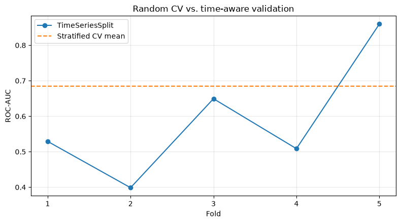
工場では未来のロットを過去データで予測します。ランダム交差検証は未来の条件を過去の学習へ混ぜるため、設備摩耗や季節変動があると性能を楽観視し得ます。
分析・モデル化の考え方
TimeSeriesSplit は時間順序を維持し、各回で過去を学習、直後の未来を検証にします。通常の層化分割と目的が異なるため、両方を用途に応じて使い分けます。
Pythonで確認する
tscv = TimeSeriesSplit(n_splits=5)
ts_rows = []
for fold, (train_idx, valid_idx) in enumerate(tscv.split(X), start=1):
    model = clone(rf_base).fit(X.iloc[train_idx], y.iloc[train_idx])
    p = model.predict_proba(X.iloc[valid_idx])[:, 1]
    ts_rows.append({
        "fold": fold,
        "train_end": df.loc[train_idx[-1], "date"].date(),
        "valid_start": df.loc[valid_idx[0], "date"].date(),
        "valid_end": df.loc[valid_idx[-1], "date"].date(),
        "valid_defect_rate": y.iloc[valid_idx].mean(),
        "roc_auc": roc_auc_score(y.iloc[valid_idx], p)
    })
ts_result = pd.DataFrame(ts_rows)
display(ts_result.round(3))

fig, ax = plt.subplots()
ax.plot(ts_result["fold"], ts_result["roc_auc"], marker="o", label="TimeSeriesSplit")
ax.axhline(cv_table["roc_auc"].mean(), color="tab:orange", linestyle="--", label="Stratified CV mean")
ax.set_title("Random CV vs. time-aware validation")
ax.set_xlabel("Fold")
ax.set_ylabel("ROC-AUC")
ax.set_xticks(ts_result["fold"])
ax.grid(True, alpha=0.3)
ax.legend()
fig.tight_layout()
plt.show()| fold | train_end | valid_start | valid_end | valid_defect_rate | roc_auc | |
|---|---|---|---|---|---|---|
| 0 | 1 | 2023-05-30 | 2023-05-31 | 2023-10-27 | 0.027 | 0.529 |
| 1 | 2 | 2023-10-27 | 2023-10-28 | 2024-03-25 | 0.047 | 0.399 |
| 2 | 3 | 2024-03-25 | 2024-03-26 | 2024-08-22 | 0.060 | 0.649 |
| 3 | 4 | 2024-08-22 | 2024-08-23 | 2025-01-19 | 0.027 | 0.509 |
| 4 | 5 | 2025-01-19 | 2025-01-20 | 2025-06-18 | 0.087 | 0.860 |
結果の読み取り
時系列分割の性能がランダム分割より低い、または後半で落ちる場合、工程条件の変化を疑います。この差は単なるモデル精度の問題ではなく、再学習頻度や監視指標を設計する材料です。
No.044:GridSearchCVでパラメータ探索する
実務での意味
木の深さや葉の最小サンプル数は、現場ノイズへの追随度を変えます。候補が少なく、重要な組み合わせを漏れなく比較したい場合にグリッド探索が適します。
分析・モデル化の考え方
探索は学習データ内の交差検証だけで行い、テストデータは触りません。今回は不良の順位付け性能を重視してROC-AUCを選択基準にします。
Pythonで確認する
param_grid = {
    "max_depth": [3, 5, 8],
    "min_samples_leaf": [4, 10, 20],
    "max_features": ["sqrt", 0.8]
}
grid = GridSearchCV(
    RandomForestClassifier(n_estimators=160, class_weight="balanced", random_state=SEED, n_jobs=-1),
    param_grid=param_grid, scoring="roc_auc", cv=cv, n_jobs=-1, return_train_score=True
)
grid.fit(X_train, y_train)
grid_top = (pd.DataFrame(grid.cv_results_)
            .sort_values("rank_test_score")
            [["rank_test_score", "mean_test_score", "std_test_score", "mean_train_score", "params"]]
            .head(5))
print("候補組み合わせ数:", len(grid.cv_results_["params"]))
print("最良パラメータ:", grid.best_params_)
display(grid_top.round(3))
候補組み合わせ数: 18
最良パラメータ: {'max_depth': 3, 'max_features': 'sqrt', 'min_samples_leaf': 10}| rank_test_score | mean_test_score | std_test_score | mean_train_score | params | |
|---|---|---|---|---|---|
| 1 | 1 | 0.694 | 0.103 | 0.960 | {'max_depth': 3, 'max_features': 'sqrt', 'min_... |
| 0 | 2 | 0.688 | 0.100 | 0.970 | {'max_depth': 3, 'max_features': 'sqrt', 'min_... |
| 13 | 3 | 0.687 | 0.124 | 0.993 | {'max_depth': 8, 'max_features': 'sqrt', 'min_... |
| 7 | 4 | 0.686 | 0.119 | 0.989 | {'max_depth': 5, 'max_features': 'sqrt', 'min_... |
| 5 | 5 | 0.680 | 0.116 | 0.936 | {'max_depth': 3, 'max_features': 0.8, 'min_sam... |
結果の読み取り
最良値だけでなく上位候補の差と標準偏差を見ます。差がごく小さいなら、浅い木や大きい葉など、単純で安定しやすい設定を採る余地があります。探索結果をテストデータで選び直さないことが重要です。
No.045:RandomizedSearchCVで探索する
実務での意味
探索候補が多い場合、全組み合わせの計算は設備・時間予算に見合わないことがあります。ランダム探索は試行数を固定し、有望な領域を広く調べます。
分析・モデル化の考え方
各パラメータの候補分布から一定回数だけ抽出します。探索の再現性を保つため random_state を固定し、グリッド探索と同じ交差検証・指標で比較します。
Pythonで確認する
param_dist = {
    "n_estimators": [100, 160, 240, 320],
    "max_depth": [3, 4, 5, 7, 9, None],
    "min_samples_split": [2, 5, 10, 20],
    "min_samples_leaf": [2, 4, 8, 12, 20],
    "max_features": ["sqrt", "log2", 0.6, 0.9]
}
random_search = RandomizedSearchCV(
    RandomForestClassifier(class_weight="balanced", random_state=SEED, n_jobs=-1),
    param_distributions=param_dist, n_iter=16, scoring="roc_auc", cv=cv,
    random_state=SEED, n_jobs=-1
)
random_search.fit(X_train, y_train)
search_compare = pd.DataFrame({
    "method": ["GridSearchCV", "RandomizedSearchCV"],
    "trials": [len(grid.cv_results_["params"]), len(random_search.cv_results_["params"])],
    "best_cv_roc_auc": [grid.best_score_, random_search.best_score_]
})
display(search_compare.round(3))
print("ランダム探索の最良パラメータ:", random_search.best_params_)| method | trials | best_cv_roc_auc | |
|---|---|---|---|
| 0 | GridSearchCV | 18 | 0.694 |
| 1 | RandomizedSearchCV | 16 | 0.694 |
ランダム探索の最良パラメータ: {'n_estimators': 160, 'min_samples_split': 10, 'min_samples_leaf': 8, 'max_features': 'log2', 'max_depth': 3}結果の読み取り
少ない試行で同程度の評価を得られれば、ランダム探索は計算効率の良い選択です。ただし偶然性があるため、候補範囲、試行回数、シードを記録し、探索自体の再現性を確保します。
No.046:過学習を確認する
実務での意味
学習データでほぼ完全でも、将来ロットで外れるモデルは検査計画に使えません。複雑さごとの学習性能と検証性能の差を確認します。
分析・モデル化の考え方
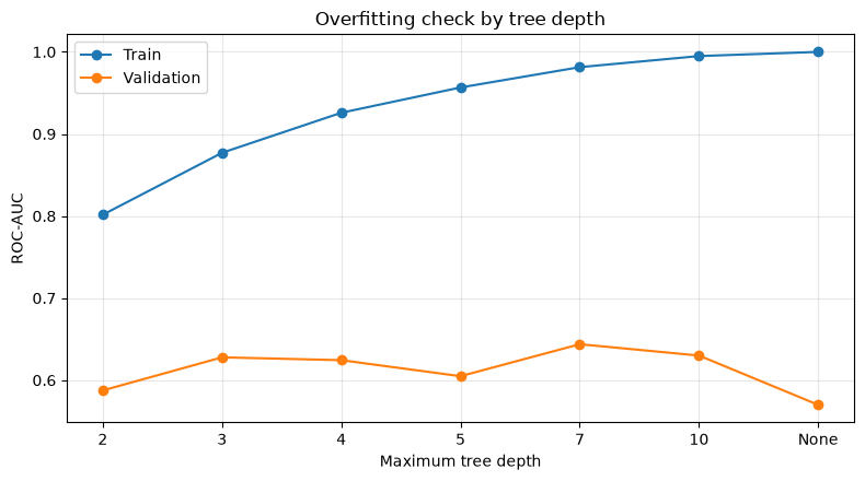
決定木の深さを増やし、学習ROC-AUCと交差検証ROC-AUCを比較します。学習値だけ上昇し検証値が頭打ち・低下する領域が過学習の兆候です。
Pythonで確認する
overfit_rows = []
for depth in [2, 3, 4, 5, 7, 10, None]:
    tree = DecisionTreeClassifier(max_depth=depth, class_weight="balanced", random_state=SEED)
    result = cross_validate(tree, X_train, y_train, cv=cv, scoring="roc_auc", return_train_score=True)
    overfit_rows.append({
        "max_depth": "None" if depth is None else str(depth),
        "train_auc": result["train_score"].mean(),
        "valid_auc": result["test_score"].mean()
    })
overfit = pd.DataFrame(overfit_rows)
display(overfit.round(3))

fig, ax = plt.subplots()
ax.plot(overfit.index, overfit["train_auc"], marker="o", label="Train")
ax.plot(overfit.index, overfit["valid_auc"], marker="o", label="Validation")
ax.set_title("Overfitting check by tree depth")
ax.set_xlabel("Maximum tree depth")
ax.set_ylabel("ROC-AUC")
ax.set_xticks(overfit.index, overfit["max_depth"])
ax.grid(True, alpha=0.3)
ax.legend()
fig.tight_layout()
plt.show()| max_depth | train_auc | valid_auc | |
|---|---|---|---|
| 0 | 2 | 0.802 | 0.587 |
| 1 | 3 | 0.877 | 0.628 |
| 2 | 4 | 0.926 | 0.624 |
| 3 | 5 | 0.957 | 0.605 |
| 4 | 7 | 0.981 | 0.644 |
| 5 | 10 | 0.995 | 0.630 |
| 6 | None | 1.000 | 0.570 |
結果の読み取り
学習線と検証線の乖離が広がる深さは避けます。対策はモデル単純化、葉の最小件数の増加、特徴量の見直し、データ追加です。製造現場では「説明できる単純さ」も採用判断に含めます。
No.047:学習曲線を確認する
実務での意味
追加データ収集には検査・ラベル付け費用がかかります。学習曲線は、データを増やす投資が性能改善につながりそうかを判断する材料です。
分析・モデル化の考え方
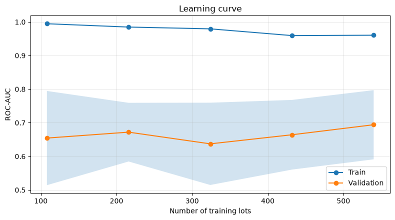
学習件数を段階的に増やし、学習と検証のROC-AUCを描きます。検証性能がまだ上向きなら追加データが有望で、両方が低位で収束するなら特徴量やモデルの見直しが先です。
Pythonで確認する
train_sizes, train_scores, valid_scores = learning_curve(
    grid.best_estimator_, X_train, y_train, cv=cv, scoring="roc_auc",
    train_sizes=np.linspace(0.2, 1.0, 5), n_jobs=-1
)
learning = pd.DataFrame({
    "train_size": train_sizes,
    "train_auc": train_scores.mean(axis=1),
    "valid_auc": valid_scores.mean(axis=1),
    "valid_std": valid_scores.std(axis=1)
})
display(learning.round(3))

fig, ax = plt.subplots()
ax.plot(train_sizes, learning["train_auc"], marker="o", label="Train")
ax.plot(train_sizes, learning["valid_auc"], marker="o", label="Validation")
ax.fill_between(train_sizes, learning["valid_auc"] - learning["valid_std"],
                learning["valid_auc"] + learning["valid_std"], alpha=0.2)
ax.set_title("Learning curve")
ax.set_xlabel("Number of training lots")
ax.set_ylabel("ROC-AUC")
ax.grid(True, alpha=0.3)
ax.legend()
fig.tight_layout()
plt.show()| train_size | train_auc | valid_auc | valid_std | |
|---|---|---|---|---|
| 0 | 108 | 0.995 | 0.654 | 0.140 |
| 1 | 216 | 0.985 | 0.672 | 0.087 |
| 2 | 324 | 0.979 | 0.637 | 0.122 |
| 3 | 432 | 0.959 | 0.664 | 0.104 |
| 4 | 540 | 0.960 | 0.694 | 0.103 |
結果の読み取り
検証曲線が終点でも上昇していれば、ロットを追加収集する価値があります。学習・検証の差が大きいままなら分散が高く、条件を網羅するデータ追加やモデル制約が必要です。曲線は因果を保証せず、収集対象の代表性も別途確認します。
No.048:特徴量重要度を確認する
実務での意味
品質技術者は、何が予測に効いているかを工程知識と照合する必要があります。重要度はセンサー改善、保全項目、追加調査の優先順位づけに使えます。
分析・モデル化の考え方
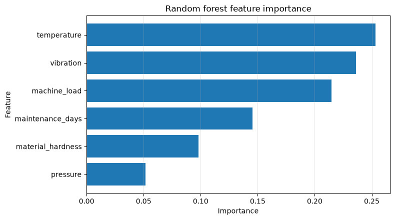
ランダムフォレストの不純度ベース重要度を確認します。これは予測への寄与方向や因果関係を示しません。相関した特徴量間では重要度が分散するため、現場知識と併用します。
Pythonで確認する
best_model = grid.best_estimator_.fit(X_train, y_train)
importance = (pd.DataFrame({"feature": features, "importance": best_model.feature_importances_})
              .sort_values("importance", ascending=True))
display(importance.sort_values("importance", ascending=False).round(3))

fig, ax = plt.subplots()
ax.barh(importance["feature"], importance["importance"])
ax.set_title("Random forest feature importance")
ax.set_xlabel("Importance")
ax.set_ylabel("Feature")
ax.grid(True, axis="x", alpha=0.3)
fig.tight_layout()
plt.show()| feature | importance | |
|---|---|---|
| 0 | temperature | 0.253 |
| 2 | vibration | 0.236 |
| 3 | machine_load | 0.215 |
| 5 | maintenance_days | 0.146 |
| 4 | material_hardness | 0.098 |
| 1 | pressure | 0.052 |
結果の読み取り
上位条件は重点監視の仮説になりますが、「値を操作すれば不良が減る」という結論には直結しません。工程試験、管理図、設備履歴などで妥当性を確認し、日付やロットIDのような代理変数が上位ならリークも疑います。
No.049:複数モデルを比較する
実務での意味
同程度の精度なら、推論速度、保守性、説明性が高いモデルの方が導入しやすいことがあります。単一指標の首位だけで決めず、複数観点を並べます。
分析・モデル化の考え方
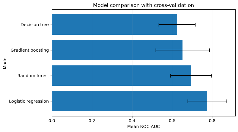
ロジスティック回帰には標準化を含むPipelineを使い、決定木、ランダムフォレスト、勾配ブースティングを同じ分割・同じ指標で比較します。
Pythonで確認する
models = {
    "Logistic regression": Pipeline([
        ("scale", StandardScaler()),
        ("model", LogisticRegression(class_weight="balanced", max_iter=1000, random_state=SEED))
    ]),
    "Decision tree": DecisionTreeClassifier(max_depth=4, class_weight="balanced", random_state=SEED),
    "Random forest": grid.best_estimator_,
    "Gradient boosting": GradientBoostingClassifier(random_state=SEED)
}
comparison_rows = []
for name, model in models.items():
    scores = cross_validate(model, X_train, y_train, cv=cv,
                            scoring={"auc": "roc_auc", "recall": "recall", "f1": "f1"}, n_jobs=-1)
    comparison_rows.append({
        "model": name,
        "roc_auc_mean": scores["test_auc"].mean(),
        "roc_auc_std": scores["test_auc"].std(),
        "recall_mean": scores["test_recall"].mean(),
        "f1_mean": scores["test_f1"].mean()
    })
model_comparison = pd.DataFrame(comparison_rows).sort_values("roc_auc_mean", ascending=False)
display(model_comparison.round(3))

fig, ax = plt.subplots()
ax.barh(model_comparison["model"], model_comparison["roc_auc_mean"],
        xerr=model_comparison["roc_auc_std"], capsize=4)
ax.set_title("Model comparison with cross-validation")
ax.set_xlabel("Mean ROC-AUC")
ax.set_ylabel("Model")
ax.grid(True, axis="x", alpha=0.3)
fig.tight_layout()
plt.show()| model | roc_auc_mean | roc_auc_std | recall_mean | f1_mean | |
|---|---|---|---|---|---|
| 0 | Logistic regression | 0.775 | 0.097 | 0.593 | 0.147 |
| 2 | Random forest | 0.694 | 0.103 | 0.413 | 0.171 |
| 3 | Gradient boosting | 0.652 | 0.134 | 0.000 | 0.000 |
| 1 | Decision tree | 0.624 | 0.091 | 0.380 | 0.153 |
結果の読み取り
平均ROC-AUC、ばらつき、再現率、F1を同時に見ます。僅差なら、説明しやすいロジスティック回帰や小さな決定木を選ぶ合理性があります。最終候補を決めた後にのみ、保留したテストデータで評価します。
No.050:実務に合う評価指標を設計する
実務での意味
不良見逃しは顧客流出や再製作につながり、過剰な重点検査は工数を増やします。両者の単価が違うため、確率閾値を0.5に固定する必然性はありません。
分析・モデル化の考え方
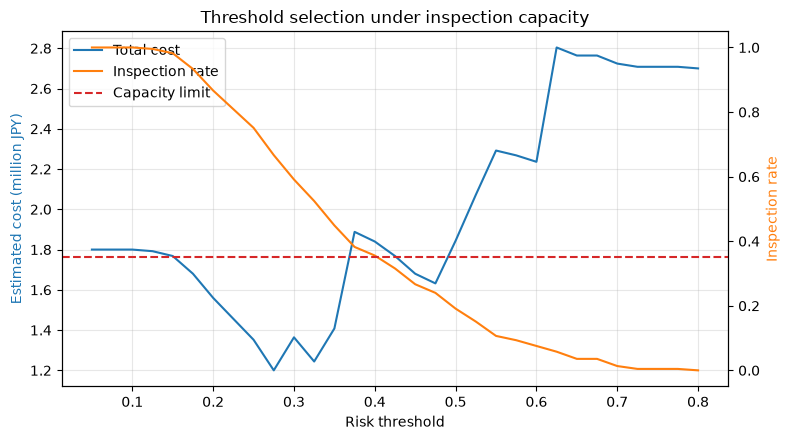
見逃し1件を30万円、重点検査1件を0.8万円とする架空の損失関数を置きます。閾値ごとに総損失と検査率を計算し、検査能力の上限35%を満たす中で最小損失を探します。実際の単価は品質保証・生産管理・営業と合意して更新します。
総損失を とします。ここで は判定閾値です。
Pythonで確認する
final_model = clone(grid.best_estimator_).fit(X_train, y_train)
test_prob = final_model.predict_proba(X_test)[:, 1]
threshold_rows = []
for threshold in np.linspace(0.05, 0.80, 31):
    pred = (test_prob >= threshold).astype(int)
    tn, fp, fn, tp = confusion_matrix(y_test, pred).ravel()
    inspection_rate = pred.mean()
    total_cost = 300_000 * fn + 8_000 * (tp + fp)
    threshold_rows.append({
        "threshold": threshold, "inspection_rate": inspection_rate,
        "recall": recall_score(y_test, pred), "false_negative": fn,
        "total_cost_yen": total_cost
    })
threshold_result = pd.DataFrame(threshold_rows)
feasible = threshold_result[threshold_result["inspection_rate"] <= 0.35]
best_policy = feasible.loc[feasible["total_cost_yen"].idxmin()]
display(best_policy.to_frame("selected_policy").round(3))

fig, ax1 = plt.subplots()
ax1.plot(threshold_result["threshold"], threshold_result["total_cost_yen"] / 1_000_000,
         color="tab:blue", label="Total cost")
ax1.set_title("Threshold selection under inspection capacity")
ax1.set_xlabel("Risk threshold")
ax1.set_ylabel("Estimated cost (million JPY)", color="tab:blue")
ax1.grid(True, alpha=0.3)
ax2 = ax1.twinx()
ax2.plot(threshold_result["threshold"], threshold_result["inspection_rate"],
         color="tab:orange", label="Inspection rate")
ax2.axhline(0.35, color="tab:red", linestyle="--", label="Capacity limit")
ax2.set_ylabel("Inspection rate", color="tab:orange")
lines = ax1.get_lines() + ax2.get_lines()
ax1.legend(lines, [line.get_label() for line in lines], loc="best")
fig.tight_layout()
plt.show()| selected_policy | |
|---|---|
| threshold | 0.475 |
| inspection_rate | 0.240 |
| recall | 0.556 |
| false_negative | 4.000 |
| total_cost_yen | 1632000.000 |
結果の読み取り
選択された閾値は、架空の損失前提と検査能力の下での候補です。ROC-AUCが同じモデルでも閾値により現場成果は変わります。本番導入では、金額だけで許容できない重大不良を別制約にし、設備・品種・顧客ごとの上限も設けます。評価用テスト件数が限られるため、損失額は点推定として過信せず、試行導入で更新します。
対象ノックを通して見える実務上の示唆
- 評価設計がモデル設計に先行する:将来を予測するなら時間順序を守り、探索用データと最終テストを分離します。
- 平均性能だけでは足りない:交差検証のばらつき、期間別性能、学習曲線から再現性を判断します。
- 最良スコアと最良業務判断は別である:説明性、検査能力、見逃しコストを含めて採用モデルと閾値を決めます。
- 特徴量重要度は仮説生成に使う:因果と断定せず、工程知識・実験・保全記録で確認します。
実務導入する場合に必要なこと
- データ定義:不良ラベル、測定タイミング、設備・品種・ロットの粒度を統一する
- リーク点検:出荷後に判明する情報や検査結果そのものを学習時の特徴量に入れない
- 評価期間:季節、設備保全、材料ロット変更を含む将来期間を確保する
- 業務指標の合意:見逃し損失、検査工数、重大不良の許容上限を部門横断で決める
- 試行運用:まず判定を参考情報として提示し、人の判断との差を記録する
- 監視と再学習:不良率、入力分布、再現率、検査率、損失を定期監視する
まとめ
No.041〜No.050では、ホールドアウトから業務損失まで、モデルを「作る」よりも重要な「正しく選び、現場で使える形にする」手順を確認しました。検証方法と評価指標は後付けではなく、何を守り、どの制約で運用するかという経営・現場の意思決定そのものです。
法人向けのご相談
数理工房では、製造データの整理、品質予測・異常検知、評価設計、PoC、本番運用を見据えたモデル監視まで、現場の制約に合わせて支援します。「データはあるが評価方法が定まらない」「精度は出たが運用判断につながらない」といった段階からご相談いただけます。
📩 お問い合わせ: surikobo.co.jp/contact
まずはお気軽にご相談ください。