Preventing Defect Outflow While Reducing Inspection Load: Model Evaluation and Verification for Manufacturing - 10 Exercises

Through hypothetical quality control cases that predict “lots to be inspected as a key point” based on manufacturing conditions, we will practice model evaluation and verification for No.041 to No.050. Instead of adopting models just because they are highly accurate, they consistently check for reproducibility to future data, validity of exploration, overlearning, explainability, and the costs of defective leakage and additional inspections.

All data, factory names, equipment names, and costs used in this article are fictional. No external data is used.

[!NOTE] This material is a notebook previously used by Surikoubo (or personally by the representative, Kazuyama), and has been reconstructed, edited, and published with the company’s permission.
All data listed is fictional and has no relation whatsoever to real companies, factories, or figures.

Introduction: Practical Challenges in Manufacturing Covered in This Article

In a hypothetical precision parts factory, inspecting every lot with the same strength creates bottlenecks in the inspection process. Therefore, we are considering a system that predicts defect risks based on factors such as temperature, pressure, vibration, and equipment load during processing, and focuses inspections on only high-risk lots.

The core of decision-making is not “which algorithm is the most accurate.” The operational questions are whether performance will be maintained in unseen future lots, defects will not be overlooked, and additional inspections will be within the on-site processing capacity.

Common situations on site

• Although the correct answer rate during development was high, performance declined in the following month’s batch
• Repeatedly selecting models with the same data, effectively fitting them into test data
• Because there are few defects, even if everything is judged as good, the correct rate appears high.
• Although the losses from missed and over-testing differ, the evaluation metric is only the correct answer rate.

Why is this issue so difficult to judge?

Evaluation values vary depending on how data is cut, chronology, class ratio, and search scope. Also, statistically good models may not match those that should be adopted in the field. Since manufacturing conditions change with equipment wear and seasons, relying solely on random division may lead to optimistic future performance.

Overview of Exercise covered this time

No.	Theme	Practical Questions
041	Holdout verification	Is performance being measured using unused data?
042	cross-validation	Does it take into account split chance?
043	TimeSeriesSplit	Verification that predicts the future from the past
044	GridSearchCV	Can you compare all candidates without missing anything?
045	RandomizedSearchCV	Can exploration budgets be allocated efficiently?
046	overlearning	Is it only suitable for training data?
047	learning curve	Does adding data work?
048	Feature Importance	What are the conditions that drive predictions?
049	Comparison of multiple models	Comparing accuracy, stability, and explainability
050	Practical Indicators	Did they compare missed cases and testing burden by price?

Preparing the Python environment

Fix the random number seed so you can reproduce the same result. Preprocessing should be included in Pipeline, and the verification data information should not be mixed into the training side. Graphs use only matplotlib.

import sys
import warnings
import numpy as np
import pandas as pd
import matplotlib
import matplotlib.pyplot as plt
import sklearn

from sklearn.base import clone
from sklearn.compose import ColumnTransformer
from sklearn.preprocessing import StandardScaler
from sklearn.pipeline import Pipeline
from sklearn.model_selection import (
    train_test_split, StratifiedKFold, TimeSeriesSplit, cross_validate,
    GridSearchCV, RandomizedSearchCV, learning_curve
)
from sklearn.metrics import (
    accuracy_score, recall_score, precision_score, f1_score, roc_auc_score,
    confusion_matrix, make_scorer
)
from sklearn.linear_model import LogisticRegression
from sklearn.tree import DecisionTreeClassifier
from sklearn.ensemble import RandomForestClassifier, GradientBoostingClassifier

warnings.filterwarnings("ignore", message="Glyph .* missing from font")
SEED = 42
np.random.seed(SEED)
plt.rcParams["figure.figsize"] = (8, 4.5)

print("Python      :", sys.version.split()[0])
print("numpy       :", np.__version__)
print("pandas      :", pd.__version__)
print("matplotlib  :", matplotlib.__version__)
print("scikit-learn:", sklearn.__version__)

Python      : 3.13.1
numpy       : 2.5.1
pandas      : 3.0.3
matplotlib  : 3.11.0
scikit-learn: 1.9.0

Creation of Fictional Data

Produces 900 days of manufacturing lots. Equipment wear progresses in the latter half, and temperatures are set to rise in summer. The probability of defects is determined by a nonlinear combination of temperature, vibration, pressure deviation, equipment load, material hardness, and wear. is_defect=1 are defective lots that you want to focus on during key inspections.

rng = np.random.default_rng(SEED)
n = 900
date = pd.date_range("2023-01-01", periods=n, freq="D")
t = np.arange(n)
temperature = 68 + 7 * np.sin(2 * np.pi * t / 365) + 0.006 * t + rng.normal(0, 2.2, n)
pressure = 100 + rng.normal(0, 4.5, n) + 0.8 * np.sin(2 * np.pi * t / 30)
vibration = np.clip(1.6 + 0.0012 * t + rng.gamma(1.8, 0.28, n), 0, None)
machine_load = np.clip(rng.normal(72, 11, n) + 5 * np.sin(2 * np.pi * t / 7), 35, 100)
material_hardness = rng.normal(61, 3.2, n)
maintenance_days = np.mod(t, 120)

logit = (-4.8 + 0.10 * (temperature - 70) + 0.60 * (vibration - 2)
         + 0.035 * np.abs(pressure - 100) + 0.028 * (machine_load - 70)
         - 0.055 * (material_hardness - 60) + 0.010 * maintenance_days
         + 0.8 * ((temperature > 75) & (machine_load > 80)))
probability = 1 / (1 + np.exp(-logit))
is_defect = rng.binomial(1, probability)

df = pd.DataFrame({
    "date": date, "temperature": temperature, "pressure": pressure,
    "vibration": vibration, "machine_load": machine_load,
    "material_hardness": material_hardness,
    "maintenance_days": maintenance_days, "is_defect": is_defect
})
features = ["temperature", "pressure", "vibration", "machine_load",
            "material_hardness", "maintenance_days"]
X, y = df[features], df["is_defect"]

display(df.head().round(2))
print(f"lot size: {len(df):,}")
print(f"Number of defective lots: {y.sum():,}(Defect rate {y.mean():.1%}）")

/var/folders/3y/fmw40k0x78xblvb3gkcyvy1h0000gn/T/ipykernel_51844/3118308666.py:29: UserWarning: obj.round has no effect with datetime, timedelta, or period dtypes. Use obj.dt.round(...) instead.
  display(df.head().round(2))

	date	temperature	pressure	vibration	machine_load	material_hardness	maintenance_days	is_defect
0	2023-01-01	68.67	101.75	2.00	61.81	61.60	0	0
1	2023-01-02	65.84	100.63	1.92	89.41	58.75	1	0
2	2023-01-03	69.90	99.66	2.05	83.81	65.58	2	0
3	2023-01-04	70.45	107.62	2.20	82.17	63.91	3	0
4	2023-01-05	64.21	97.79	2.03	82.93	61.93	4	0

Lot size: 900
Number of defective lots: 38 (defect rate 4.2%)

First, check for changes in time series and class imbalance. The monthly defect rate fluctuates because the number of parameters is small, but it is clear that the conditions become stricter in the latter half.

monthly = df.set_index("date")["is_defect"].resample("MS").agg(["mean", "count"])
fig, ax = plt.subplots()
ax.plot(monthly.index, monthly["mean"], marker="o", linewidth=1.5)
ax.set_title("Monthly defect rate (synthetic data)")
ax.set_xlabel("Month")
ax.set_ylabel("Defect rate")
ax.grid(True, alpha=0.3)
fig.tight_layout()
plt.show()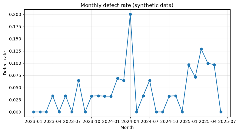

No.041: Conducting Holdout Verification

Meaning in Practice

Test data not used for model creation is secured and evaluated as a simulated production before implementation. For quality applications, to maintain defect rates, the defects are stratified and divided by objective variables.

Approach to Analysis and Modeling

Here, 25% of the total is reserved for testing. If you repeatedly change models or thresholds to match test results, test data can be mixed with training, so the final check should only be done once.

Check with Python

X_train, X_test, y_train, y_test = train_test_split(
    X, y, test_size=0.25, stratify=y, random_state=SEED
)
rf_base = RandomForestClassifier(
    n_estimators=200, max_depth=5, min_samples_leaf=8,
    class_weight="balanced", random_state=SEED, n_jobs=-1
)
rf_base.fit(X_train, y_train)
holdout_prob = rf_base.predict_proba(X_test)[:, 1]
holdout_pred = (holdout_prob >= 0.5).astype(int)
holdout_result = pd.Series({
    "train_rows": len(X_train), "test_rows": len(X_test),
    "accuracy": accuracy_score(y_test, holdout_pred),
    "recall": recall_score(y_test, holdout_pred),
    "precision": precision_score(y_test, holdout_pred),
    "roc_auc": roc_auc_score(y_test, holdout_prob)
})
display(holdout_result.to_frame("value").round(3))
display(pd.DataFrame(confusion_matrix(y_test, holdout_pred),
                     index=["actual_good", "actual_defect"],
                     columns=["pred_good", "pred_defect"]))

	value
train_rows	675.000
test_rows	225.000
accuracy	0.849
recall	0.333
precision	0.097
roc_auc	0.748

	pred_good	pred_defect
actual_good	188	28
actual_defect	6	3

Reading the results

In addition to the correct answer rate, we also list the recall rate, which indicates how many actual defects were detected, and the ROC-AUC, which indicates ranking capability. The lower left of the mixed line is the one I missed. In practice, the quality assurance department checks whether this number of cases is within an acceptable range.

No.042: Perform cross-verification

Meaning in Practice

The evaluation value obtained from a single split is influenced by chance. Cross-validation allows performance and variation to be measured across multiple virtual test intervals.

Approach to Analysis and Modeling

Use StratifiedKFold to roughly match the defect rate for each installment. It shows not only the mean but also the standard deviation, helping to understand the uncertainty of model selection.

If the five-division rating is set to $s_1,\ldots,s_5$, you will check the mean $\bar{s}=\frac{1}{5}\sum_{i=1}^{5}s_i$ and standard deviation.

Check with Python

cv = StratifiedKFold(n_splits=5, shuffle=True, random_state=SEED)
cv_scores = cross_validate(
    rf_base, X, y, cv=cv,
    scoring={"roc_auc": "roc_auc", "recall": "recall", "f1": "f1"},
    n_jobs=-1
)
cv_table = pd.DataFrame({
    name.replace("test_", ""): values
    for name, values in cv_scores.items() if name.startswith("test_")
})
display(cv_table.round(3))
display(cv_table.agg(["mean", "std"]).round(3))

	roc_auc	recall	f1
0	0.602	0.286	0.133
1	0.784	0.571	0.267
2	0.649	0.125	0.077
3	0.659	0.375	0.194
4	0.727	0.500	0.229

	roc_auc	recall	f1
mean	0.684	0.371	0.180
std	0.071	0.177	0.076

Reading the results

Models with good averages but large standard deviations are unstable depending on the composition of target lots. If the recall rate fluctuates significantly between segments, consider adding defective samples, reviewing process-specific models, and evaluating the period.

No.043: Using TimeSeriesSplit

Meaning in Practice

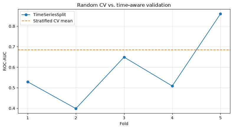
At the factory, future lots are predicted using historical data. Random cross-validation mixes future conditions with past learning, so performance can be optimistic when equipment wear or seasonal fluctuations occur.

Approach to Analysis and Modeling

TimeSeriesSplit maintains chronological order, learning from the past each session and verifying the immediate future. Since the purpose differs from regular layered segmentation, both are used according to the intended use.

Check with Python

tscv = TimeSeriesSplit(n_splits=5)
ts_rows = []
for fold, (train_idx, valid_idx) in enumerate(tscv.split(X), start=1):
    model = clone(rf_base).fit(X.iloc[train_idx], y.iloc[train_idx])
    p = model.predict_proba(X.iloc[valid_idx])[:, 1]
    ts_rows.append({
        "fold": fold,
        "train_end": df.loc[train_idx[-1], "date"].date(),
        "valid_start": df.loc[valid_idx[0], "date"].date(),
        "valid_end": df.loc[valid_idx[-1], "date"].date(),
        "valid_defect_rate": y.iloc[valid_idx].mean(),
        "roc_auc": roc_auc_score(y.iloc[valid_idx], p)
    })
ts_result = pd.DataFrame(ts_rows)
display(ts_result.round(3))

fig, ax = plt.subplots()
ax.plot(ts_result["fold"], ts_result["roc_auc"], marker="o", label="TimeSeriesSplit")
ax.axhline(cv_table["roc_auc"].mean(), color="tab:orange", linestyle="--", label="Stratified CV mean")
ax.set_title("Random CV vs. time-aware validation")
ax.set_xlabel("Fold")
ax.set_ylabel("ROC-AUC")
ax.set_xticks(ts_result["fold"])
ax.grid(True, alpha=0.3)
ax.legend()
fig.tight_layout()
plt.show()

	fold	train_end	valid_start	valid_end	valid_defect_rate	roc_auc
0	1	2023-05-30	2023-05-31	2023-10-27	0.027	0.529
1	2	2023-10-27	2023-10-28	2024-03-25	0.047	0.399
2	3	2024-03-25	2024-03-26	2024-08-22	0.060	0.649
3	4	2024-08-22	2024-08-23	2025-01-19	0.027	0.509
4	5	2025-01-19	2025-01-20	2025-06-18	0.087	0.860

Reading the results

If the performance of time-series segmentation is lower than random partitioning or drops in the latter half, we suspect changes in process conditions. This difference is not just a matter of model accuracy, but also the material used to design retraining frequency and monitoring metrics.

No.044: Searching for Parameters in GridSearchCV

Meaning in Practice

The depth of the tree and the minimum number of leaf samples affect the degree to which on-site noise is followed. Grid exploration is suitable when there are few candidates and you want to compare important combinations without omission.

Approach to Analysis and Modeling

Exploration is performed only through cross-validation within the training data; test data is not touched. This time, we prioritize defect ranking performance and use ROC-AUC as the selection criterion.

Check with Python

param_grid = {
    "max_depth": [3, 5, 8],
    "min_samples_leaf": [4, 10, 20],
    "max_features": ["sqrt", 0.8]
}
grid = GridSearchCV(
    RandomForestClassifier(n_estimators=160, class_weight="balanced", random_state=SEED, n_jobs=-1),
    param_grid=param_grid, scoring="roc_auc", cv=cv, n_jobs=-1, return_train_score=True
)
grid.fit(X_train, y_train)
grid_top = (pd.DataFrame(grid.cv_results_)
            .sort_values("rank_test_score")
            [["rank_test_score", "mean_test_score", "std_test_score", "mean_train_score", "params"]]
            .head(5))
print("Number of candidate combinations:", len(grid.cv_results_["params"]))
print("Best parameters:", grid.best_params_)
display(grid_top.round(3))

Number of candidate combinations: 18
Best parameters: {'max_depth': 3, 'max_features': 'sqrt', 'min_samples_leaf': 10}

	rank_test_score	mean_test_score	std_test_score	mean_train_score	params
1	1	0.694	0.103	0.960	{'max_depth': 3, 'max_features': 'sqrt', 'min_...
0	2	0.688	0.100	0.970	{'max_depth': 3, 'max_features': 'sqrt', 'min_...
13	3	0.687	0.124	0.993	{'max_depth': 8, 'max_features': 'sqrt', 'min_...
7	4	0.686	0.119	0.989	{'max_depth': 5, 'max_features': 'sqrt', 'min_...
5	5	0.680	0.116	0.936	{'max_depth': 3, 'max_features': 0.8, 'min_sam...

Reading the results

We look not only at the best values but also at the differences and standard deviations among top contenders. If the difference is very small, there is room to adopt simple, stable settings such as shallow trees or large leaves. It is important not to reselect search results based on test data.

No.045: Searching with RandomizedSearchCV

Meaning in Practice

If there are many search candidates, calculating all combinations may not fit the equipment and time budget. Random search fixes the number of trials and broadly explores promising areas.

Approach to Analysis and Modeling

A certain number of times are extracted from the candidate distribution of each parameter. To maintain reproducibility in exploration, random_state is fixed and compared using the same cross-validation and metrics as grid searches.

Check with Python

param_dist = {
    "n_estimators": [100, 160, 240, 320],
    "max_depth": [3, 4, 5, 7, 9, None],
    "min_samples_split": [2, 5, 10, 20],
    "min_samples_leaf": [2, 4, 8, 12, 20],
    "max_features": ["sqrt", "log2", 0.6, 0.9]
}
random_search = RandomizedSearchCV(
    RandomForestClassifier(class_weight="balanced", random_state=SEED, n_jobs=-1),
    param_distributions=param_dist, n_iter=16, scoring="roc_auc", cv=cv,
    random_state=SEED, n_jobs=-1
)
random_search.fit(X_train, y_train)
search_compare = pd.DataFrame({
    "method": ["GridSearchCV", "RandomizedSearchCV"],
    "trials": [len(grid.cv_results_["params"]), len(random_search.cv_results_["params"])],
    "best_cv_roc_auc": [grid.best_score_, random_search.best_score_]
})
display(search_compare.round(3))
print("Best parameters for random search:", random_search.best_params_)

	method	trials	best_cv_roc_auc
0	GridSearchCV	18	0.694
1	RandomizedSearchCV	16	0.694

Best parameters for random search: {'n_estimators': 160, 'min_samples_split': 10, 'min_samples_leaf': 8, 'max_features': 'log2', 'max_depth': 3}

Reading the results

If you can achieve the same rating with fewer attempts, random search is a computationally efficient choice. However, due to the nature of chance, we record the range of candidates, number of trials, and seeds to ensure reproducibility of the exploration itself.

No.046: Checking for Overlearning

Meaning in Practice

Even if the training data is nearly complete, models that fail in future batch sizes cannot be used for inspection planning. We will examine the differences in learning and validation performance for each complexity.

Approach to Analysis and Modeling

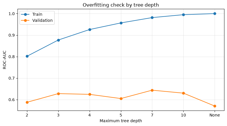
Increase the depth of decision trees and compare the learning ROC-AUC with cross-validation ROC-AUC. A sign of overlearning is a region where only the learning value rises while the validation value plateaus or falls.

Check with Python

overfit_rows = []
for depth in [2, 3, 4, 5, 7, 10, None]:
    tree = DecisionTreeClassifier(max_depth=depth, class_weight="balanced", random_state=SEED)
    result = cross_validate(tree, X_train, y_train, cv=cv, scoring="roc_auc", return_train_score=True)
    overfit_rows.append({
        "max_depth": "None" if depth is None else str(depth),
        "train_auc": result["train_score"].mean(),
        "valid_auc": result["test_score"].mean()
    })
overfit = pd.DataFrame(overfit_rows)
display(overfit.round(3))

fig, ax = plt.subplots()
ax.plot(overfit.index, overfit["train_auc"], marker="o", label="Train")
ax.plot(overfit.index, overfit["valid_auc"], marker="o", label="Validation")
ax.set_title("Overfitting check by tree depth")
ax.set_xlabel("Maximum tree depth")
ax.set_ylabel("ROC-AUC")
ax.set_xticks(overfit.index, overfit["max_depth"])
ax.grid(True, alpha=0.3)
ax.legend()
fig.tight_layout()
plt.show()

	max_depth	train_auc	valid_auc
0	2	0.802	0.587
1	3	0.877	0.628
2	4	0.926	0.624
3	5	0.957	0.605
4	7	0.981	0.644
5	10	0.995	0.630
6	None	1.000	0.570

Reading the results

Avoid the depth where the gap between the learning and verification lines widens. Countermeasures include model simplification, increasing the minimum number of leaves, reviewing features, and adding data. In manufacturing sites, “simplicity that can be explained” is also included in hiring decisions.

No.047: Check the learning curve

Meaning in Practice

Additional data collection incurs testing and labeling costs. The learning curve is a key factor in determining whether investing in increased data is likely to lead to improved performance.

Approach to Analysis and Modeling

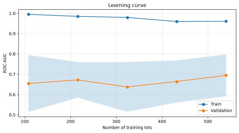
Gradually increase the number of training sessions and draw the ROC-AUC for learning and validation. If verification performance is still improving, additional data is promising; if both converge at low levels, reviewing features and models should come first.

Check with Python

train_sizes, train_scores, valid_scores = learning_curve(
    grid.best_estimator_, X_train, y_train, cv=cv, scoring="roc_auc",
    train_sizes=np.linspace(0.2, 1.0, 5), n_jobs=-1
)
learning = pd.DataFrame({
    "train_size": train_sizes,
    "train_auc": train_scores.mean(axis=1),
    "valid_auc": valid_scores.mean(axis=1),
    "valid_std": valid_scores.std(axis=1)
})
display(learning.round(3))

fig, ax = plt.subplots()
ax.plot(train_sizes, learning["train_auc"], marker="o", label="Train")
ax.plot(train_sizes, learning["valid_auc"], marker="o", label="Validation")
ax.fill_between(train_sizes, learning["valid_auc"] - learning["valid_std"],
                learning["valid_auc"] + learning["valid_std"], alpha=0.2)
ax.set_title("Learning curve")
ax.set_xlabel("Number of training lots")
ax.set_ylabel("ROC-AUC")
ax.grid(True, alpha=0.3)
ax.legend()
fig.tight_layout()
plt.show()

	train_size	train_auc	valid_auc	valid_std
0	108	0.995	0.654	0.140
1	216	0.985	0.672	0.087
2	324	0.979	0.637	0.122
3	432	0.959	0.664	0.104
4	540	0.960	0.694	0.103

Reading the results

If the validation curve is rising even at the end, it is worth collecting additional lots. If the gap between training and validation remains large, variance is high, requiring additional data and model constraints covering all conditions. Curves do not guarantee causality, and the representativeness of the collected items is checked separately.

No.048: Checking the Importance of Features

Meaning in Practice

Quality engineers need to compare what is effective for predictions against process knowledge. Importance can be used to prioritize sensor improvements, maintenance items, and additional investigations.

Approach to Analysis and Modeling

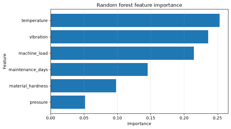
Check the impurity and importance of random forests. This does not indicate the direction of contribution or causality to the forecast. Since the importance of correlated features varies, it is used together with field knowledge.

Check with Python

best_model = grid.best_estimator_.fit(X_train, y_train)
importance = (pd.DataFrame({"feature": features, "importance": best_model.feature_importances_})
              .sort_values("importance", ascending=True))
display(importance.sort_values("importance", ascending=False).round(3))

fig, ax = plt.subplots()
ax.barh(importance["feature"], importance["importance"])
ax.set_title("Random forest feature importance")
ax.set_xlabel("Importance")
ax.set_ylabel("Feature")
ax.grid(True, axis="x", alpha=0.3)
fig.tight_layout()
plt.show()

	feature	importance
0	temperature	0.253
2	vibration	0.236
3	machine_load	0.215
5	maintenance_days	0.146
4	material_hardness	0.098
1	pressure	0.052

Reading the results

The higher-level condition is the focused monitoring hypothesis, but it does not directly lead to the conclusion that “manipulating values reduces defects.” Validity is confirmed through process tests, control charts, and equipment history, and if proxy variables like dates or lot IDs are high, leaks are suspected.

No.049: Comparing Multiple Models

Meaning in Practice

For similar accuracy, models with high inference speed, maintainability, and explainability may be easier to implement. Instead of determining the top of a single indicator, multiple perspectives are considered.

Approach to Analysis and Modeling

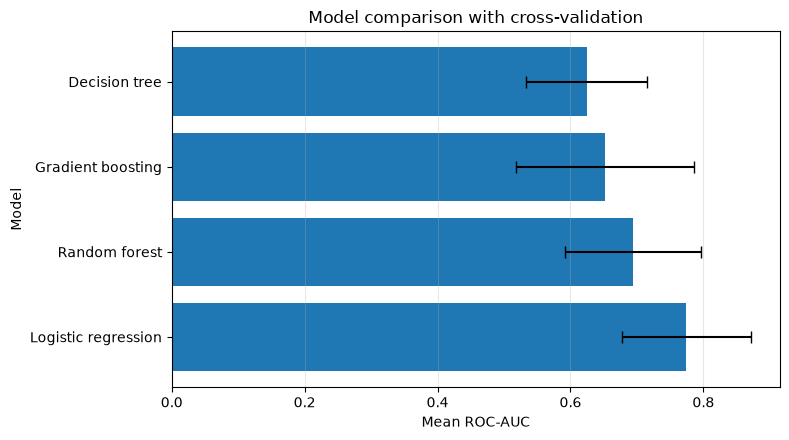
For logistic regression, we use a pipeline that includes standardization, comparing decision trees, random forests, and gradient boosting using the same splits and metrics.

Check with Python

models = {
    "Logistic regression": Pipeline([
        ("scale", StandardScaler()),
        ("model", LogisticRegression(class_weight="balanced", max_iter=1000, random_state=SEED))
    ]),
    "Decision tree": DecisionTreeClassifier(max_depth=4, class_weight="balanced", random_state=SEED),
    "Random forest": grid.best_estimator_,
    "Gradient boosting": GradientBoostingClassifier(random_state=SEED)
}
comparison_rows = []
for name, model in models.items():
    scores = cross_validate(model, X_train, y_train, cv=cv,
                            scoring={"auc": "roc_auc", "recall": "recall", "f1": "f1"}, n_jobs=-1)
    comparison_rows.append({
        "model": name,
        "roc_auc_mean": scores["test_auc"].mean(),
        "roc_auc_std": scores["test_auc"].std(),
        "recall_mean": scores["test_recall"].mean(),
        "f1_mean": scores["test_f1"].mean()
    })
model_comparison = pd.DataFrame(comparison_rows).sort_values("roc_auc_mean", ascending=False)
display(model_comparison.round(3))

fig, ax = plt.subplots()
ax.barh(model_comparison["model"], model_comparison["roc_auc_mean"],
        xerr=model_comparison["roc_auc_std"], capsize=4)
ax.set_title("Model comparison with cross-validation")
ax.set_xlabel("Mean ROC-AUC")
ax.set_ylabel("Model")
ax.grid(True, axis="x", alpha=0.3)
fig.tight_layout()
plt.show()

	model	roc_auc_mean	roc_auc_std	recall_mean	f1_mean
0	Logistic regression	0.775	0.097	0.593	0.147
2	Random forest	0.694	0.103	0.413	0.171
3	Gradient boosting	0.652	0.134	0.000	0.000
1	Decision tree	0.624	0.091	0.380	0.153

Reading the results

View average ROC-AUC, variation, recall, and F1 all at once. If the margin is narrow, there is rationality to choose easy-to-explain logistic regression or small decision trees. Only after finalists are selected will the pending test data be evaluated.

No.050: Designing Evaluation Indicators Fit for Practical Work

Meaning in Practice

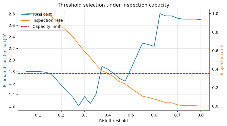
Missing defects leads to customer loss and reproduction, while excessive focused inspections increase man-hours. Since the unit prices of the two are different, there is no necessity to fix the probability threshold at 0.5.

Approach to Analysis and Modeling

We set a hypothetical loss function where one missed case is worth 300,000 yen and one key inspection case is 8,000 yen. For each threshold, calculate total loss and inspection rate, and find the minimum loss while meeting the 35% inspection cap. Actual unit prices are updated in agreement with quality assurance, production management, and sales.

Let the total loss be $C(t)=300{,}000\,FN(t)+8{,}000\{TP(t)+FP(t)\}$. Here, $t$ is the threshold for judgment.

Check with Python

final_model = clone(grid.best_estimator_).fit(X_train, y_train)
test_prob = final_model.predict_proba(X_test)[:, 1]
threshold_rows = []
for threshold in np.linspace(0.05, 0.80, 31):
    pred = (test_prob >= threshold).astype(int)
    tn, fp, fn, tp = confusion_matrix(y_test, pred).ravel()
    inspection_rate = pred.mean()
    total_cost = 300_000 * fn + 8_000 * (tp + fp)
    threshold_rows.append({
        "threshold": threshold, "inspection_rate": inspection_rate,
        "recall": recall_score(y_test, pred), "false_negative": fn,
        "total_cost_yen": total_cost
    })
threshold_result = pd.DataFrame(threshold_rows)
feasible = threshold_result[threshold_result["inspection_rate"] <= 0.35]
best_policy = feasible.loc[feasible["total_cost_yen"].idxmin()]
display(best_policy.to_frame("selected_policy").round(3))

fig, ax1 = plt.subplots()
ax1.plot(threshold_result["threshold"], threshold_result["total_cost_yen"] / 1_000_000,
         color="tab:blue", label="Total cost")
ax1.set_title("Threshold selection under inspection capacity")
ax1.set_xlabel("Risk threshold")
ax1.set_ylabel("Estimated cost (million JPY)", color="tab:blue")
ax1.grid(True, alpha=0.3)
ax2 = ax1.twinx()
ax2.plot(threshold_result["threshold"], threshold_result["inspection_rate"],
         color="tab:orange", label="Inspection rate")
ax2.axhline(0.35, color="tab:red", linestyle="--", label="Capacity limit")
ax2.set_ylabel("Inspection rate", color="tab:orange")
lines = ax1.get_lines() + ax2.get_lines()
ax1.legend(lines, [line.get_label() for line in lines], loc="best")
fig.tight_layout()
plt.show()

	selected_policy
threshold	0.475
inspection_rate	0.240
recall	0.556
false_negative	4.000
total_cost_yen	1632000.000

Reading the results

The selected thresholds are candidates under hypothetical loss assumptions and inspection capabilities. Even with the same ROC-AUC model, field outcomes vary depending on the threshold. For full-scale implementation, we set separate restrictions for serious defects that cannot be tolerated by price alone, and set upper limits for each equipment, type, and customer. Since the number of evaluation tests is limited, the loss amount is not overestimated as a point estimate and is updated through trial implementation.

Practical Implications Seen Through Target Exercise

1. Evaluation design takes precedence over model design: If you are forecasting the future, follow chronological order and separate exploration data from final tests.
2. Average performance alone is not enough.: Variation in cross-validation, performance by period, and learning curve are used to determine reproducibility.
3. The best score and the best business judgment are separate: Determine adoption models and thresholds, including explainability, inspection capability, and missed cut costs.
4. Feature importance is used for hypothesis generation: Confirm without definitive causality, using process knowledge, experiments, and maintenance records.

What is necessary for practical implementation

• Data definition: Standardize defective labels, measurement timing, equipment, varieties, and lot grit sizes
• Leak Inspection: Information and inspection results discovered after shipment cannot be included in the characteristics during training.
• Evaluation period: Secure future periods including seasons, equipment maintenance, and material lot changes.
• Agreement on business metrics: Set the allowable limits for missed losses, inspection work, and major defects across departments
• trial operation: First, present judgments as reference information and record the differences from others’ judgments.
• Monitoring and Relearning: Regularly monitor defect rates, input distributions, recall rates, inspection rates, and losses.

Conclusion

From No.041 to No.050, we reviewed the steps for “correctly selecting and making it usable on site,” which is more important than simply “making” models, from holdout to operational losses. Verification methods and evaluation indicators are not retroactive; they are the very decisions made by management and the field about what to follow and under what constraints to implement.

Consultations for Corporations

At Surikoubou, we support everything from organizing manufacturing data, quality prediction and anomaly detection, evaluation design, PoC, to model monitoring for production operations, tailored to on-site constraints. You can consult from the stage where “we have data but can’t decide on an evaluation method” or “accuracy is achieved but it doesn’t lead to operational decisions.”

📩 Contact Us: surikobo.co.jp/contact
Please feel free to consult us first.