Making Quality Forecasting a ‘System Usable on the Floor’: 10 Lightweight MLOps Practices in Manufacturing

In this article, we will use a hypothetical model that predicts defect risks based on machining conditions to continuously review the necessary After modeling aspects such as storage, inference, on-site provision, monitoring, relearning, and project management. The target is No.091 to No.100.

Not only analytical accuracy but also designing who uses it, when, and for what, and how to stop it in case of abnormalities is essential for establishing it in manufacturing environments.

[!NOTE] This material is a notebook previously used by Surikoubo (or personally by the representative, Kazuyama), and has been reconstructed, edited, and published with the company’s permission. All data listed is fictional and has no relation whatsoever to real companies, factories, or figures.

Introduction: Practical Challenges in Manufacturing Covered in This Article

At one parts factory, a prototype model was developed to predict in-process defects based on temperature, pressure, vibration, and cycle time. However, it only operates in the manager’s notebook and cannot be used by manufacturing engineers for daily lot determination. In this article, we will resolve the situation of “having a model but not actually working out.”

Common situations on site

• Column order and preprocessing during training are not reproduced during inference
• There is no usage path for bulk CSV checks, saving results, screens/APIs, etc.
• Who detects accuracy decline by which metric and when to relearn is undefined
• When models are misjudged, the boundaries between on-site responsibility, quality assurance, and IT become unclear.

Why is this issue so difficult to judge?

The value of machine learning is not determined by accuracy alone. Missed losses, verification man-hours, response times, uptime, data quality, and explainability must be handled simultaneously. Furthermore, if process conditions or material lots change, the relationships established during learning may not necessarily continue in the future.

Overview of Exercise covered this time

No.	Theme	Practical deliverables
091–093	Save, Read, and Inference Functions	Reproducible inference components
094–095	Batch Inference & CSV Export	Daily Judgment File
096–098	API, Screen, Dashboard	Delivery routes by user
099	Relearning Timing	Monitoring Rules and Decision Tables
100	How the Project Proceeds	Phased Implementation Roadmap

This time, we will combine preprocessing and models into Pipeline to prevent processing differences between training and inference.

Preparing the Python environment

Load the main library and fix the random number seed. To avoid environment-dependent garbled text, the Japanese graph is displayed in English.

from pathlib import Path
import ast
import json
import platform
import joblib
import matplotlib
import matplotlib.pyplot as plt
import numpy as np
import pandas as pd
import sklearn
from IPython.display import display
from sklearn.compose import ColumnTransformer
from sklearn.ensemble import RandomForestClassifier
from sklearn.metrics import classification_report, confusion_matrix, roc_auc_score
from sklearn.model_selection import train_test_split
from sklearn.pipeline import Pipeline
from sklearn.preprocessing import OneHotEncoder, StandardScaler

SEED = 42
rng = np.random.default_rng(SEED)
ARTIFACT_DIR = Path("artifacts_10")
ARTIFACT_DIR.mkdir(exist_ok=True)
pd.set_option("display.max_columns", 20)
print({"python": platform.python_version(), "pandas": pd.__version__,
       "scikit-learn": sklearn.__version__, "matplotlib": matplotlib.__version__})

{'python': '3.13.1', 'pandas': '3.0.3', 'scikit-learn': '1.9.0', 'matplotlib': '3.11.0'}

Creation of Fictional Data

We produce 1,200 lots using three different facilities. The defect rate is set to increase during high temperature, high vibration, long cycles, old equipment M-03, and night shifts. This is not proof of causality, but rather fictitious data intended to concretize future operational designs.

n = 1200
df = pd.DataFrame({
    "lot_id": [f"LOT-{i:05d}" for i in range(1, n + 1)],
    "timestamp": pd.date_range("2025-01-01", periods=n, freq="2h"),
    "machine_id": rng.choice(["M-01", "M-02", "M-03"], n, p=[0.4, 0.35, 0.25]),
    "shift": rng.choice(["day", "night"], n, p=[0.65, 0.35]),
    "temperature_c": rng.normal(180, 7, n),
    "pressure_mpa": rng.normal(5.2, 0.45, n),
    "vibration_mm_s": rng.gamma(3.0, 0.55, n),
    "cycle_time_s": rng.normal(48, 4, n),
})
logit = (-4.0 + 0.085*(df.temperature_c-180) + 0.75*(df.vibration_mm_s-1.5)
         + 0.07*(df.cycle_time_s-48) + 0.55*(df.machine_id == "M-03")
         + 0.30*(df.shift == "night") + 0.15*np.abs(df.pressure_mpa-5.2))
prob = 1 / (1 + np.exp(-logit))
df["is_defect"] = rng.binomial(1, prob)
print(f"rows={len(df):,}, defect_rate={df.is_defect.mean():.1%}")
display(df.head())

rows=1,200, defect_rate=4.8%

	lot_id	timestamp	machine_id	shift	temperature_c	pressure_mpa	vibration_mm_s	cycle_time_s	is_defect
0	LOT-00001	2025-01-01 00:00:00	M-03	day	184.560784	4.865795	2.390549	51.370749	0
1	LOT-00002	2025-01-01 02:00:00	M-02	day	184.351209	4.666892	1.968884	44.359844	0
2	LOT-00003	2025-01-01 04:00:00	M-03	night	179.739255	5.665214	3.724858	51.636246	0
3	LOT-00004	2025-01-01 06:00:00	M-02	night	181.382894	4.433155	1.622987	47.156151	0
4	LOT-00005	2025-01-01 08:00:00	M-01	day	171.703708	5.617085	0.746812	46.240817	0

feature_cols = ["machine_id", "shift", "temperature_c", "pressure_mpa",
                "vibration_mm_s", "cycle_time_s"]
categorical_cols = ["machine_id", "shift"]
numeric_cols = [c for c in feature_cols if c not in categorical_cols]
X_train, X_test, y_train, y_test = train_test_split(
    df[feature_cols], df["is_defect"], test_size=0.25,
    random_state=SEED, stratify=df["is_defect"])
preprocess = ColumnTransformer([
    ("num", StandardScaler(), numeric_cols),
    ("cat", OneHotEncoder(handle_unknown="ignore"), categorical_cols),
])
model = Pipeline([
    ("preprocess", preprocess),
    ("classifier", RandomForestClassifier(n_estimators=160, min_samples_leaf=5,
                                           class_weight="balanced", random_state=SEED, n_jobs=-1)),
])
model.fit(X_train, y_train)
test_prob = model.predict_proba(X_test)[:, 1]
print(f"test ROC-AUC: {roc_auc_score(y_test, test_prob):.3f}")

test ROC-AUC: 0.654

No.091: Saving a Trained Model

Meaning in Practice

By fixing validated models as deliverables, the same logic can be reused without opening the trainer’s notebook. For audits and bug investigations, the model body and metadata are managed in pairs.

Approach to Analysis and Modeling

Save the Pipeline that integrates preprocessing and classifiers in joblib. It also records features, thresholds, training dates, library versions, and evaluation values, making it possible to track “what was saved.”

Check with Python

MODEL_PATH = ARTIFACT_DIR / "defect_risk_pipeline_v1.joblib"
META_PATH = ARTIFACT_DIR / "defect_risk_pipeline_v1.json"
joblib.dump(model, MODEL_PATH)
metadata = {"model_version": "1.0.0", "trained_at": "2025-04-15T09:00:00+09:00",
            "features": feature_cols, "threshold": 0.35,
            "test_roc_auc": round(float(roc_auc_score(y_test, test_prob)), 4),
            "sklearn_version": sklearn.__version__, "seed": SEED}
META_PATH.write_text(json.dumps(metadata, ensure_ascii=False, indent=2), encoding="utf-8")
print(MODEL_PATH, f"{MODEL_PATH.stat().st_size/1024:.1f} KiB")
print(META_PATH.read_text(encoding="utf-8"))

artifacts_10/defect_risk_pipeline_v1.joblib 877.0 KiB
{
  "model_version": "1.0.0",
  "trained_at": "2025-04-15T09:00:00+09:00",
  "features": [
    "machine_id",
    "shift",
    "temperature_c",
    "pressure_mpa",
    "vibration_mm_s",
    "cycle_time_s"
  ],
  "threshold": 0.35,
  "test_roc_auc": 0.6541,
  "sklearn_version": "1.9.0",
  "seed": 42
}

Reading the results

Not only the model file but also thresholds and features are left in JSON, preventing confusion in judgment conditions. In practice, Git adds commit ID, training data duration, approvers, and data definition versions.

No.092: Loading Saved Models

Meaning in Practice

Batches and servers on the manufacturing floor do not re-execute the learning process but load approved deliverables. Checking health at startup helps detect misdeployments early.

Approach to Analysis and Modeling

After loading, check the type, expected step name, and inference in the few records. joblib is dangerous if it loads untrusted files, so limit it to internal management areas and consider checking hashes.

Check with Python

loaded_model = joblib.load(MODEL_PATH)
loaded_meta = json.loads(META_PATH.read_text(encoding="utf-8"))
assert list(loaded_model.named_steps) == ["preprocess", "classifier"]
smoke_prob = loaded_model.predict_proba(X_test.head(3))[:, 1]
display(pd.DataFrame({"model_version": loaded_meta["model_version"],
                      "defect_probability": smoke_prob.round(4)}))

	model_version	defect_probability
0	1.0.0	0.3970
1	1.0.0	0.2748
2	1.0.0	0.2073

Reading the results

I received the same input format before and after saving, and the probability was restored. In the deployment pipeline, in addition to this smoke test, the match with expected values for known inputs is also automatically tested.

No.093: Creating Inference Functions

Meaning in Practice

Without making the user aware of the internal model details, input verification, probability calculation, threshold determination, and version information assignment are consolidated into a single contract.

Approach to Analysis and Modeling

If the probability is $\hat{p}(y=1\mid x)$ and the threshold is $t$, the alert is $\mathbb{1}[\hat{p}\ge t]$. Thresholds are determined not by maximizing accuracy, but by missed losses and verification capability.

Check with Python

def predict_defect(records, fitted_model=loaded_model, meta=loaded_meta):
    frame = pd.DataFrame(records).copy()
    missing = sorted(set(meta["features"]) - set(frame.columns))
    if missing:
        raise ValueError(f"missing columns: {missing}")
    probabilities = fitted_model.predict_proba(frame[meta["features"]])[:, 1]
    return frame.assign(defect_probability=probabilities,
                        alert=(probabilities >= meta["threshold"]).astype(int),
                        model_version=meta["model_version"])

sample = X_test.head(5).to_dict(orient="records")
display(predict_defect(sample))

	machine_id	shift	temperature_c	pressure_mpa	vibration_mm_s	cycle_time_s	defect_probability	alert	model_version
0	M-02	night	168.681284	5.803114	3.031016	48.535739	0.396985	1	1.0.0
1	M-01	day	167.631267	5.822293	1.519621	53.958552	0.274760	0	1.0.0
2	M-01	day	179.984248	5.807577	1.319119	44.209292	0.207304	0	1.0.0
3	M-03	day	168.900776	5.039525	0.966915	45.571332	0.007375	0	1.0.0
4	M-03	day	190.531547	5.347335	1.389076	50.565215	0.717243	1	1.0.0

Reading the results

Probability, conditioning, and model versions are now available for function return values, making downstream processes easier to handle. In practice, numerical ranges, nulls, category candidates, and units are also verified, and errors are logged.

No.094: Batch Inference on CSV

Meaning in Practice

In sites where daily CSVs are generated from MES or inspection equipment, introducing batch inference before APIs makes it easier to connect to existing operations.

Approach to Analysis and Modeling

Input IDs are matched one-to-one with predictions to check for duplicate IDs, missing columns, and row number changes. This time, we create a CSV simulating an undetermined 40 lots, load it, and infer after loading.

Check with Python

batch_input = df.loc[X_test.index[:40], ["lot_id", "timestamp"] + feature_cols].copy()
INPUT_CSV = ARTIFACT_DIR / "daily_lots.csv"
batch_input.to_csv(INPUT_CSV, index=False)
incoming = pd.read_csv(INPUT_CSV)
assert incoming["lot_id"].is_unique
assert set(feature_cols).issubset(incoming.columns)
batch_scored = predict_defect(incoming[feature_cols]).copy()
batch_scored.insert(0, "lot_id", incoming["lot_id"])
batch_scored.insert(1, "timestamp", incoming["timestamp"])
print(f"input={len(incoming)}, output={len(batch_scored)}, alerts={batch_scored.alert.sum()}")
display(batch_scored.head())

input=40, output=40, alerts=7

	lot_id	timestamp	machine_id	shift	temperature_c	pressure_mpa	vibration_mm_s	cycle_time_s	defect_probability	alert	model_version
0	LOT-00412	2025-02-04 06:00:00	M-02	night	168.681284	5.803114	3.031016	48.535739	0.396985	1	1.0.0
1	LOT-00587	2025-02-18 20:00:00	M-01	day	167.631267	5.822293	1.519621	53.958552	0.274760	0	1.0.0
2	LOT-00140	2025-01-12 14:00:00	M-01	day	179.984248	5.807577	1.319119	44.209292	0.207304	0	1.0.0
3	LOT-01174	2025-04-08 18:00:00	M-03	day	168.900776	5.039525	0.966915	45.571332	0.007375	0	1.0.0
4	LOT-00431	2025-02-05 20:00:00	M-03	day	190.531547	5.347335	1.389076	50.565215	0.717243	1	1.0.0

Reading the results

The number of input and output lines matched, and we obtained the lot number that required confirmation. During operation, file name rules, character encoding, prevention of double registration upon rerun, and recovery in case of intermediate failures are also determined.

No.095: Exporting Forecast Results to CSV

Meaning in Practice

To pass forecasts to on-site reports or BI, it is necessary to retain not only probabilities but also judgments, model versions, and processing times. This is also used for later quality tracking.

Approach to Analysis and Modeling

Fix the output schema, save it, then reload it to verify the number of entries and required columns. The probability is maintained while only the digits on display are retained.

Check with Python

OUTPUT_CSV = ARTIFACT_DIR / "daily_lots_scored.csv"
export_cols = ["lot_id", "timestamp", "defect_probability", "alert", "model_version"]
export_df = batch_scored[export_cols].copy()
export_df["scored_at"] = "2025-04-16T06:00:00+09:00"
export_df.to_csv(OUTPUT_CSV, index=False, float_format="%.6f")
check = pd.read_csv(OUTPUT_CSV)
assert len(check) == len(incoming) and set(export_df.columns) == set(check.columns)
print(f"saved: {OUTPUT_CSV} ({OUTPUT_CSV.stat().st_size:,} bytes)")
display(check.sort_values("defect_probability", ascending=False).head())

saved: artifacts_10/daily_lots_scored.csv (2,986 bytes)

	lot_id	timestamp	defect_probability	alert	model_version	scored_at
4	LOT-00431	2025-02-05 20:00:00	0.717243	1	1.0.0	2025-04-16T06:00:00+09:00
38	LOT-00036	2025-01-03 22:00:00	0.576321	1	1.0.0	2025-04-16T06:00:00+09:00
28	LOT-00014	2025-01-02 02:00:00	0.563290	1	1.0.0	2025-04-16T06:00:00+09:00
27	LOT-00994	2025-03-24 18:00:00	0.508810	1	1.0.0	2025-04-16T06:00:00+09:00
29	LOT-00286	2025-01-24 18:00:00	0.435847	1	1.0.0	2025-04-16T06:00:00+09:00

Reading the results

You can submit the high-risk confirmation list as a CSV. However, this does not mean ‘alert=1 means defect is confirmed.’ It is used as a priority for additional inspections, and the final decision and response history are separately recorded.

No.096: Creating an Inference API with FastAPI

Meaning in Practice

When calling in real time from facility apps or MES, HTTP APIs clarify contracts between systems. Fixed input and output formats allow multiple systems to use the same model.

Approach to Analysis and Modeling

Define the input type in Pydantic and load the model only once at startup. Authentication, TLS, timeouts, rate limits, and audit logs are requirements that should be added for production.

Check with Python

api_source = r'''from fastapi import FastAPI
from pydantic import BaseModel
import joblib
import pandas as pd

app = FastAPI(title="Defect Risk API", version="1.0.0")
model = joblib.load("defect_risk_pipeline_v1.joblib")

class Lot(BaseModel):
    machine_id: str
    shift: str
    temperature_c: float
    pressure_mpa: float
    vibration_mm_s: float
    cycle_time_s: float

@app.get("/health")
def health():
    return {"status": "ok", "model_version": "1.0.0"}

@app.post("/predict")
def predict(lot: Lot):
    frame = pd.DataFrame([lot.model_dump()])
    probability = float(model.predict_proba(frame)[0, 1])
    return {"defect_probability": probability, "alert": probability >= 0.35}
'''
ast.parse(api_source)
(ARTIFACT_DIR / "api_app.py").write_text(api_source, encoding="utf-8")
print("FastAPI sample syntax: OK")

FastAPI sample syntax: OK

Reading the results

I was able to syntax verify the minimum API contract. Notebook does not start the server. Before production, testing for normal systems, boundary values, missing values, and simultaneous access, as well as a system to safely roll back the model, are necessary.

No.097: Creating a Simple Screen with Streamlit

Meaning in Practice

If field personnel cannot directly handle CSV or APIs, the simplified screen lowers barriers to PoC usage and allows operational requirements to be discovered in a short time.

Approach to Analysis and Modeling

The input fields show the unit, acceptable range, and initial value, and the result is shown as a set of probability and next action. Screens are not a substitute for formal quality evaluation systems, but rather a means of step-by-step verification for implementation.

Check with Python

streamlit_source = r'''import streamlit as st
import joblib
import pandas as pd

st.title("Processing lot Defect Risk Confirmation")
model = joblib.load("defect_risk_pipeline_v1.joblib")
machine = st.selectbox("Equipment", ["M-01", "M-02", "M-03"])
shift = st.selectbox("Work Schedule", ["day", "night"])
temperature = st.number_input("temperature (°C)", 150.0, 210.0, 180.0)
pressure = st.number_input("pressure (MPa)", 3.0, 7.0, 5.2)
vibration = st.number_input("vibration (mm/s)", 0.0, 10.0, 1.5)
cycle = st.number_input("cycle time (s)", 30.0, 70.0, 48.0)
if st.button("Judgment"):
    x = pd.DataFrame([{"machine_id": machine, "shift": shift,
        "temperature_c": temperature, "pressure_mpa": pressure,
        "vibration_mm_s": vibration, "cycle_time_s": cycle}])
    p = float(model.predict_proba(x)[0, 1])
    st.metric("Defective Risk", f"{p:.1%}")
    st.warning("Recommendation of additional tests") if p >= 0.35 else st.success("normal flow")
'''
ast.parse(streamlit_source)
(ARTIFACT_DIR / "streamlit_app.py").write_text(streamlit_source, encoding="utf-8")
print("Streamlit sample syntax: OK")

Streamlit sample syntax: OK

Reading the results

From input to action suggestions, everything is consolidated into one screen. In implementation evaluation, users observe the input they are hesitant about, actions taken after judgment, and processing time, reflecting these into the requirements of the formal system.

No.098: Dashboardizing Forecast Results

Meaning in Practice

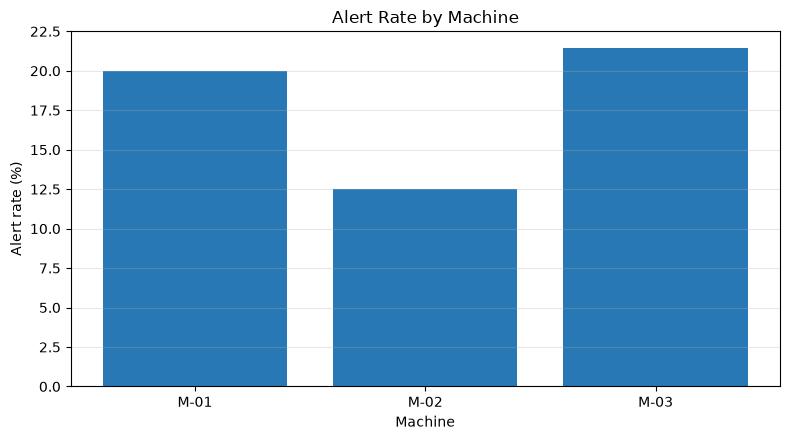
Managers need not only individual records but also warning rates for each facility, time changes, and processing volume. We identify biases and connect them to conservation, condition adjustment, and the assignment of verification personnel.

Approach to Analysis and Modeling

The warning rate is the percentage of the model’s output, not the defect rate itself. The number of units is listed alongside the numbers, and it is read along with changes in equipment and product configuration.

Check with Python

dash = batch_scored.groupby("machine_id").agg(
    lots=("lot_id", "size"), alert_rate=("alert", "mean"),
    mean_risk=("defect_probability", "mean")).sort_index()
display(dash.style.format({"alert_rate": "{:.1%}", "mean_risk": "{:.1%}"}))
fig, ax = plt.subplots(figsize=(8, 4.5))
ax.bar(dash.index, dash["alert_rate"] * 100, color="#2878B5")
ax.set_title("Alert Rate by Machine")
ax.set_xlabel("Machine")
ax.set_ylabel("Alert rate (%)")
ax.grid(axis="y", alpha=0.3)
plt.tight_layout()
plt.show()

	lots	alert_rate	mean_risk
machine_id
M-01	10	20.0%	26.3%
M-02	16	12.5%	16.9%
M-03	14	21.4%	21.9%

Reading the results

It provides an overview of the difference in warning rates between facilities. However, since it is a small sample of 40 cases, it cannot be immediately concluded that it is an equipment malfunction. We stratify by product, material, and work area, and determine the investigation priority after matching actual defects.

No.099: Designing the Model Retraining Timing

Meaning in Practice

When materials, equipment, conditions, and inspection standards change, the model deteriorates. Regular relearning alone can cause you to miss changes that are too fast, and conversely, unnecessary updates increase the verification load.

Approach to Analysis and Modeling

Input drift and predictive performance are monitored separately. The Population Stability Index is set from the standard ratio of $e_i$ and the current ratio of $a_i$ to $PSI=\sum_i(a_i-e_i)\ln(a_i/e_i)$ for each section. PSI is a signal of change, not proof of deterioration.

Check with Python

def psi(expected, actual, bins=10):
    edges = np.unique(np.quantile(expected, np.linspace(0, 1, bins + 1)))
    edges[0], edges[-1] = -np.inf, np.inf
    e = np.histogram(expected, bins=edges)[0] / len(expected)
    a = np.histogram(actual, bins=edges)[0] / len(actual)
    e, a = np.clip(e, 1e-6, None), np.clip(a, 1e-6, None)
    return float(np.sum((a - e) * np.log(a / e)))

current_temp = rng.normal(185, 7, 400)  # Assuming conditions after the change in conditions
temp_psi = psi(X_train["temperature_c"].to_numpy(), current_temp)
monitor = pd.DataFrame({
    "signal": ["temperature PSI", "30-day ROC-AUC", "missing rate", "new machine"],
    "observed": [round(temp_psi, 3), 0.68, 0.012, 1],
    "trigger": [0.20, 0.70, 0.01, 1],
    "action": ["investigate/retrain", "retrain review", "stop and fix data", "revalidate"]})
monitor["triggered"] = [temp_psi >= .20, .68 < .70, .012 > .01, True]
display(monitor)

	signal	observed	trigger	action	triggered
0	temperature PSI	0.504	0.20	investigate/retrain	True
1	30-day ROC-AUC	0.680	0.70	retrain review	True
2	missing rate	0.012	0.01	stop and fix data	True
3	new machine	1.000	1.00	revalidate	True

Reading the results

Multiple triggers ignited. Instead of automatically and immediately replacing them, we conduct root cause investigation→ relearning→ comparing with past models→ quality officer approval→ and phased releases. Delays in the arrival of correct labels are also incorporated into the monitoring design.

No.100: Organize how to proceed with a machine learning project

Meaning in Practice

Practical implementation is not just about model development. We agree on phased matters including target determination, business changes, data collection, system connectivity, education, and monitoring.

Approach to Analysis and Modeling

First, set business KPIs and withdrawal conditions, then reduce risk in the order of offline verification, shadow operations, limited operations, and production deployment. Cost-effectiveness is continuously evaluated using “defect reduction amount - additional inspection costs - operating costs.”

Check with Python

roadmap = pd.DataFrame([
    ["1. Issue Definition", "Missed Loss Detection Ability -KPIAgreed", "Quality Assurance/Manufacturing/Management", "2 weeks"],
    ["2. Data Verification", "Check definitions, missing points, timing, and leaks", "ManufacturingIT/Analysis", "3 weeks"],
    ["3. Offline Verification", "Comparing Reference Methods and Candidate Models", "Analysis/Quality Assurance", "3 weeks"],
    ["4. Shadow Operations", "Recording with real data instead of using it for judgment", "On-site/Analysis", "4 weeks"],
    ["5. Limited operation", "1Facilities &1Supporting additional inspections with products", "site manager", "4 weeks"],
    ["6. Sex and Surveillance", "SLAMonitoring, relearning, and stopping procedures", "IT/Quality Assurance", "continuous"],
], columns=["phase", "exit_criteria", "owner", "duration"])
display(roadmap)
print("Total pilot lead time:", sum([2, 3, 3, 4, 4]), "weeks")

	phase	exit_criteria	owner	duration
0	1. Issue Definition	Missed Loss Detection Ability -KPIAgreed	Quality Assurance/Manufacturing/Management	2 weeks
1	2. Data Verification	Check definitions, missing points, timing, and leaks	ManufacturingIT/Analysis	3 weeks
2	3. Offline Verification	Comparing Reference Methods and Candidate Models	Analysis/Quality Assurance	3 weeks
3	4. Shadow Operations	Recording with real data instead of using it for judgment	On-site/Analysis	4 weeks
4	5. Limited operation	1Facilities &1Supporting additional inspections with products	site manager	4 weeks
5	6. Sex and Surveillance	SLAMonitoring, relearning, and stopping procedures	IT/Quality Assurance	continuous

Total pilot lead time: 16 weeks

Reading the results

This is a pilot example of about 16 weeks. By assigning completion conditions and responsible persons to each stage, we prevent ‘accuracy is achieved but not used.’ If business KPIs do not improve due to limited operations, we review thresholds, business workflows, and issue settings.

Practical Implications Seen Through Target Exercise

1. Reproducibility cannot be created by models alone.: Manage preprocessing, feature definition, thresholds, and plate information together.
2. Users choose their delivery routes: For daily tasks, CSV is suitable; for system integration, APIs; and for initial verification, simple screens are suitable.
3. Separating Forecasting and Decision-Making: The model indicates risks, and responsibility for inspections, stoppages, and condition changes lies with business rules.
4. Monitoring is input, output, correct answers, and operations.KPIThe four layers: Retraining is not automatically determined based on a single metric.

What is necessary for practical implementation

• Clearly state the handling of data dictionaries, units, acquisition points, and losses
• Considering the costs of missed incidents and false alarms, consider thresholds for each equipment and product
• Organize model ledgers, access control, audit logs, backups, and rollbacks
• Agree on RACI responsible for on-site, quality assurance, manufacturing technology, IT, and analytics.
• Confirm safety and operational effectiveness through shadow operations, and clearly specify shutdown conditions.

Conclusion

From No.091 to No.100, we changed the system to allow trained models to be “usable, trackable, and stopped.” The starting point for lightweight MLOps is not a large-scale foundation, but reproducible deliverables, clear inputs and outputs, phased implementation, monitoring, and separation of responsibilities. Operations that review technical metrics and on-site KPIs in the same meeting lead to ongoing value.

Consultations for Corporations

At Mathematical Laboratory, we support everything from manufacturing data inventory, prediction and anomaly detection PoC, embedding into existing systems, operational monitoring design, to in-house training, tailored to the maturity of the site.

📩 Contact Us: surikobo.co.jp/contact Please feel free to consult us first.