Capturing Equipment Abnormalities “Before Stopping”: Detection of Abnormalities and Alert Design at the Manufacturing Site - 10 Exercises

In this article, we will thoroughly check the Definition of anomalies, statistical detection, multivariate detection using machine learning, and alert design that can be operated in the field from 10 bottles No.071 to No.080, focusing on the temperature, vibration, current, and pressure of manufacturing equipment. The goal is not to test algorithms, but to create a system that allows maintenance personnel to decide “when, what, and at what priority” to check.

[!NOTE] This material is a notebook previously used by Surikoubo (or personally by the representative, Kazuyama), and has been reconstructed, edited, and published with the company’s permission.
All data listed is fictional and has no relation whatsoever to real companies, factories, or figures.

Introduction: Practical Challenges in Manufacturing Covered in This Article

To reduce equipment outages, predictive maintenance that detects state changes early is essential, not just recovery after failures. On the other hand, tightening thresholds increases alerts, while loosening them causes critical anomalies to be missed. In this paper, we generate sensor data for 30 days and 720 hours of sensor data for a single hypothetical processing device, considering implementation from both detection accuracy and response cost perspectives.

Common situations on site

• Even with normal load fluctuations, temperature and current rise, and at fixed thresholds, false positives are common.
• Momentary spikes, gradual degradation, and multi-sensor combination abnormalities are all mixed together.
• Only the number of alerts increases, and it’s unclear who will check when.
• Few correct labels, making it difficult to evaluate accuracy

Why is this issue so difficult to judge?

“Abnormal values” and “dangerous conditions as equipment” are not the same. The normal range varies depending on product type, load, startup/stop, and ambient temperature. Additionally, false positives waste inspection man-hours, and missed ones lead to downtime losses and safety risks, so simple correct accuracy cannot be used for evaluation. It is necessary to design detection models, business rules, and response flows as a unified solution.

Overview of Exercise covered this time

No.	Theme	Key Points to Use for Judgment
071	Types of Outliers	Distinguishing Point, Context, and Set Anomalies
072–074	Statistical Detection	Use univariate, robust statistics, and time variation appropriately
075–077	Machine Learning	Learning boundaries in situations with few correct labels
078–079	Multivariate and visualization	Supporting inter-sensor relationships and on-site verification
080	Alert Design	Adjusting for false positives and missed detections at cost

Preparing the Python environment

Handle data with numpy and pandas, and visualize it with matplotlib. scikit-learn is used for anomaly detection models. For reproducibility, random number seeds are fixed and do not depend on external data.

import sys
import warnings
import numpy as np
import pandas as pd
import matplotlib
import matplotlib.pyplot as plt
import japanize_matplotlib

from sklearn.ensemble import IsolationForest
from sklearn.neighbors import LocalOutlierFactor
from sklearn.svm import OneClassSVM
from sklearn.preprocessing import StandardScaler
from sklearn.metrics import confusion_matrix, precision_score, recall_score, f1_score

warnings.filterwarnings("ignore", category=UserWarning)
SEED = 42
rng = np.random.default_rng(SEED)
pd.set_option("display.max_columns", 20)
pd.set_option("display.float_format", "{:.2f}".format)

print("Python      :", sys.version.split()[0])
print("numpy       :", np.__version__)
print("pandas      :", pd.__version__)
print("matplotlib  :", matplotlib.__version__)

Python      : 3.13.1
numpy       : 2.5.1
pandas      : 3.0.3
matplotlib  : 3.11.0

Creation of Fictional Data

Creating hourly conditions for processing equipment M-01. load_pct changes in response to load factor, bearing temperature, vibration, spindle current, and hydraulic pressure. To check the correct answer, the following artificial anomalies are mixed in.

• Point anomaly: Temporary temperature and vibration spikes
• contextual anomaly: Only the current is excessive relative to the load
• set anomaly: Temperature and vibration worsen over several tens of hours
• multivariate anomaly: Individual values are not extreme, but the combination of temperature, vibration, and pressure is unnatural

In actual operation, is_anomaly is unknown. In this article, I will keep it for method comparison only.

n = 24 * 30
ts = pd.date_range("2025-04-01", periods=n, freq="h")
hour = np.arange(n)
load = np.clip(68 + 15 * np.sin(2 * np.pi * hour / 24) + rng.normal(0, 6, n), 25, 100)

df = pd.DataFrame({
    "timestamp": ts,
    "load_pct": load,
    "temperature_c": 41 + 0.20 * load + rng.normal(0, 1.1, n),
    "vibration_mm_s": 0.9 + 0.018 * load + rng.normal(0, 0.14, n),
    "current_a": 8 + 0.34 * load + rng.normal(0, 1.2, n),
    "pressure_mpa": 5.5 - 0.006 * load + rng.normal(0, 0.08, n),
    "anomaly_type": "normal",
})

def mark(idx, kind):
    df.loc[idx, "anomaly_type"] = kind

point_idx = np.array([95, 188, 422, 611])
df.loc[point_idx, "temperature_c"] += [9, 12, 10, 11]
df.loc[point_idx, "vibration_mm_s"] += [1.1, 1.5, 1.2, 1.4]
mark(point_idx, "point")

context_idx = np.arange(270, 278)
df.loc[context_idx, "current_a"] += 9
mark(context_idx, "contextual")

collective_idx = np.arange(500, 536)
ramp = np.linspace(0.5, 7.5, len(collective_idx))
df.loc[collective_idx, "temperature_c"] += ramp
df.loc[collective_idx, "vibration_mm_s"] += ramp * 0.11
mark(collective_idx, "collective")

multi_idx = np.arange(650, 660)
df.loc[multi_idx, "temperature_c"] += 4.0
df.loc[multi_idx, "vibration_mm_s"] += 0.55
df.loc[multi_idx, "pressure_mpa"] -= 0.28
mark(multi_idx, "multivariate")

df["is_anomaly"] = (df["anomaly_type"] != "normal").astype(int)
print("Data Shape:", df.shape)
display(df.head())
display(df.groupby("anomaly_type").size().rename("hours").to_frame())

Data Format: (720, 8)

	timestamp	load_pct	temperature_c	vibration_mm_s	current_a	pressure_mpa	anomaly_type	is_anomaly
0	2025-04-01 00:00:00	69.83	54.86	2.06	31.12	5.11	normal	0
1	2025-04-01 01:00:00	65.64	55.37	2.13	29.19	5.18	normal	0
2	2025-04-01 02:00:00	80.00	54.49	2.15	36.76	5.08	normal	0
3	2025-04-01 03:00:00	84.25	56.20	2.62	37.41	5.09	normal	0
4	2025-04-01 04:00:00	69.28	53.84	2.13	32.28	5.08	normal	0

	hours
anomaly_type
collective	36
contextual	8
multivariate	10
normal	662
point	4

No.071: Organizing Types of Outliers

Meaning in Practice

If you don’t distinguish between types of abnormalities, you may use methods that are resistant to single-shot spikes to look for gradual deterioration, causing the purpose and means to be mismatched. Point abnormalities are treated as sensor failures or shocks, contextual abnormalities as mismatches with load or type, and cluster abnormalities as continuous degradation.

Approach to Analysis and Modeling

Each abnormal section is summarized by duration and maximum temperature. Not only whether you have exceeded the “usual range,” but how long it has lasted affects the decision to stop.

Check with Python

type_summary = (df.groupby("anomaly_type")
                  .agg(hours=("timestamp", "size"),
                       max_temperature_c=("temperature_c", "max"),
                       max_vibration_mm_s=("vibration_mm_s", "max"),
                       mean_current_a=("current_a", "mean"))
                  .sort_values("hours", ascending=False))
display(type_summary.round(2))

	hours	max_temperature_c	max_vibration_mm_s	mean_current_a
anomaly_type
normal	662	62.85	2.94	30.96
collective	36	65.47	3.45	31.51
multivariate	10	63.64	3.11	35.36
contextual	8	60.68	2.53	42.62
point	4	65.48	3.45	28.00

Reading the results

Point anomalies have short durations but large peaks, while collective anomalies last 36 hours. For example, the former involves immediate confirmation, while the latter involves trend monitoring and planned maintenance, serving as a basis for changing response deadlines for each type of anomaly.

No.072: Detecting Anomalies with Z-Score

Meaning in Practice

The Z-score is a primary screening that shows how many standard deviations the current value deviates from the past average and is easy to explain.

Approach to Analysis and Modeling

$x$ temperature is , mean $\mu$, and standard deviation $\sigma$, $z=(x-\mu)/\sigma$. Here, $|z|>3$ is considered an anomaly candidate. However, it is important to note that the mean and standard deviation themselves are affected by outliers.

Check with Python

mu = df["temperature_c"].mean()
sigma = df["temperature_c"].std(ddof=0)
df["z_score"] = (df["temperature_c"] - mu) / sigma
df["pred_z"] = (df["z_score"].abs() > 3).astype(int)

z_result = df.loc[df["pred_z"] == 1,
                  ["timestamp", "temperature_c", "z_score", "anomaly_type"]]
print(f"average={mu:.2f}℃, standard deviation={sigma:.2f}℃, Detection={len(z_result)}records")
display(z_result.head(10).round(2))

Average=54.86°C, Standard Deviation=2.99°C, Detection=4 entries

	timestamp	temperature_c	z_score	anomaly_type
531	2025-04-23 03:00:00	63.96	3.05	collective
533	2025-04-23 05:00:00	65.47	3.55	collective
535	2025-04-23 07:00:00	65.07	3.42	collective
611	2025-04-26 11:00:00	65.48	3.56	point

Reading the results

Large temperature spikes can be picked up with fewer rules. On the other hand, normal high temperatures linked to loads or contextual anomalies caused by current alone cannot be evaluated. The Z-score serves as a baseline for monitoring clear deviations from a single sensor.

No.073: Detecting Anomalies with IQR

Meaning in Practice

When sudden anomalies push up the mean or standard deviation, IQR, which is close to the median, can serve as a robust fixed threshold.

Approach to Analysis and Modeling

Let the first quartile be $Q_1$, the third quartile $Q_3$, and $IQR=Q_3-Q_1$. $[Q_1-1.5IQR,\ Q_3+1.5IQR]$ is the outside of the candidate.

Check with Python

q1, q3 = df["vibration_mm_s"].quantile([0.25, 0.75])
iqr = q3 - q1
lower, upper = q1 - 1.5 * iqr, q3 + 1.5 * iqr
df["pred_iqr"] = ((df["vibration_mm_s"] < lower) |
                  (df["vibration_mm_s"] > upper)).astype(int)

print(f"IQR={iqr:.3f}, lower limit={lower:.3f}, upper limit={upper:.3f}, Detection={df['pred_iqr'].sum()}records")
display(df.loc[df["pred_iqr"] == 1,
               ["timestamp", "vibration_mm_s", "anomaly_type"]].head(10).round(3))

IQR=0.375, Lower Limit=1.368, Upper Limit=2.869, Detection=19 Cases

	timestamp	vibration_mm_s	anomaly_type
176	2025-04-08 08:00:00	2.94	normal
188	2025-04-08 20:00:00	3.29	point
422	2025-04-18 14:00:00	3.32	point
509	2025-04-22 05:00:00	2.97	collective
529	2025-04-23 01:00:00	3.17	collective
530	2025-04-23 02:00:00	2.90	collective
531	2025-04-23 03:00:00	2.91	collective
532	2025-04-23 04:00:00	3.08	collective
533	2025-04-23 05:00:00	3.45	collective
535	2025-04-23 07:00:00	3.39	collective

Reading the results

Extreme increases in vibrations can be detected relatively unaffected by distortions in the distribution. However, since vibration changes caused by load are not considered, it is necessary to have standards for different conditions at sites where the product type and operating conditions differ significantly.

No.074: Detecting Anomalies by Deviations from Moving Averages

Meaning in Practice

Even if the standard values differ for each facility, changes from your “most recent self” can be monitored. This method is suitable for gradually changing states or local changes.

Approach to Analysis and Modeling

Calculate the moving average and moving standard deviation over the past 24 hours without including the current value. By excluding the current value in the baseline calculation, the impact of anomalies simultaneously pushing up the threshold is minimized.

Check with Python

past_temp = df["temperature_c"].shift(1)
df["temp_ma24"] = past_temp.rolling(24, min_periods=12).mean()
df["temp_sd24"] = past_temp.rolling(24, min_periods=12).std()
df["rolling_score"] = ((df["temperature_c"] - df["temp_ma24"]) /
                       df["temp_sd24"].clip(lower=0.3))
df["pred_rolling"] = (df["rolling_score"] > 3).astype(int)

fig, ax = plt.subplots(figsize=(12, 4))
window = df.iloc[470:550]
ax.plot(window["timestamp"], window["temperature_c"], label="temperature", linewidth=1.5)
ax.plot(window["timestamp"], window["temp_ma24"], label="past24time average", linewidth=2)
flag = window[window["pred_rolling"] == 1]
ax.scatter(flag["timestamp"], flag["temperature_c"], color="crimson", label="Detection", zorder=3)
ax.set_title("Temperature and moving average in set anomaly intervals")
ax.set_xlabel("Date and Time")
ax.set_ylabel("Bearing temperature (℃）")
ax.grid(True, alpha=0.3)
ax.legend()
fig.tight_layout()
plt.show()
print("Number of Detected Cases:", int(df["pred_rolling"].sum()))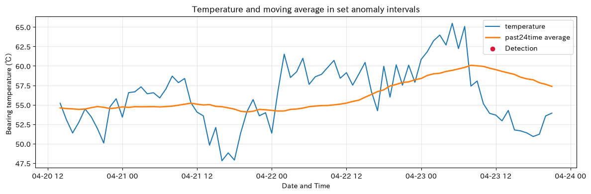

Number of detections: 2

Reading the results

It can detect a rise at the start of deterioration, but if the rise continues for a long time, the moving averages will follow, making it harder to detect. Practical use is to combine short-term deviation detection with long-term trend tilt monitoring.

No.075: Using Isolation Forest

Meaning in Practice

Monitoring can be performed without manually breaking down multiple sensor combinations into numerous thresholds. It can also be used during the startup phase when there are few abnormal labels.

Approach to Analysis and Modeling

Isolation Forest uses random segmentation to separate small or isolated observations along short paths. Here, we use four sensors and load rates, and set the anomaly rate assumption as contamination=0.08. This value is adjusted based on the number of inspectable cases, not the “true abnormality rate.”

Check with Python

features = ["load_pct", "temperature_c", "vibration_mm_s", "current_a", "pressure_mpa"]
X = df[features]
iso = IsolationForest(n_estimators=300, contamination=0.08, random_state=SEED)
iso.fit(X)
df["score_iso"] = -iso.score_samples(X)
df["pred_iso"] = (iso.predict(X) == -1).astype(int)

iso_metrics = {
    "Number of Detected Cases": int(df["pred_iso"].sum()),
    "Compatibility rate": precision_score(df["is_anomaly"], df["pred_iso"]),
    "recall rate": recall_score(df["is_anomaly"], df["pred_iso"]),
    "F1": f1_score(df["is_anomaly"], df["pred_iso"]),
}
display(pd.Series(iso_metrics, name="Isolation Forest").to_frame().T.round(3))

	Number of Detected Cases	Compatibility rate	recall rate	F1
Isolation Forest	58.00	0.52	0.52	0.52

Reading the results

It can detect combinations of sensors that are difficult to detect under univariate rules. Not only recall but also accuracy is checked to determine whether the inspection staff can handle the number of cases. If training data contains many anomalies, boundaries become distorted, so it is desirable to train during stable operation periods.

No.076: Using Local Outlier Factor

Meaning in Practice

When normal conditions are divided into multiple operating modes, LOF (Field of Defense) is effective, which looks at the density difference with neighboring areas rather than the entire data.

Approach to Analysis and Modeling

LOF treats observations with lower local density compared to nearby points as anomalies. Standardization is essential because distance is used. If the n_neighbors is too small, it is sensitive to noise; if too large, it loses sight of local structure.

Check with Python

Xs = StandardScaler().fit_transform(X)
lof = LocalOutlierFactor(n_neighbors=30, contamination=0.08)
df["pred_lof"] = (lof.fit_predict(Xs) == -1).astype(int)
df["score_lof"] = -lof.negative_outlier_factor_

display(pd.DataFrame({
    "technique": ["LOF"],
    "Number of Detected Cases": [int(df["pred_lof"].sum())],
    "Compatibility rate": [precision_score(df["is_anomaly"], df["pred_lof"])],
    "recall rate": [recall_score(df["is_anomaly"], df["pred_lof"])],
    "F1": [f1_score(df["is_anomaly"], df["pred_lof"])],
}).round(3))

	technique	Number of Detected Cases	Compatibility rate	recall rate	F1
0	LOF	58	0.71	0.71	0.71

Reading the results

LOF picks up locally rare conditions, but if abnormal sections are clustered together, it may be judged normal because “abnormalities are close together.” To sequentially judge new data, separate normal training data and inference data into novelty=True.

No.077: Using One-Class SVM

Meaning in Practice

Flexible boundaries are created from normally functioning samples to detect states that deviate from “normality.” It is suitable for equipment that can clearly secure normal data.

Approach to Analysis and Modeling

The RBF kernel represents a nonlinear normal region. nu relates to the upper limit of the percentage of learning points outside the boundary, while gamma determines the fineness of the boundary. Here, training is based on known normal data, but in practice, the stability period is chosen based on maintenance records.

Check with Python

scaler_oc = StandardScaler()
X_normal = scaler_oc.fit_transform(df.loc[df["is_anomaly"] == 0, features])
X_all = scaler_oc.transform(X)
ocsvm = OneClassSVM(kernel="rbf", nu=0.05, gamma="scale")
ocsvm.fit(X_normal)
df["pred_ocsvm"] = (ocsvm.predict(X_all) == -1).astype(int)
df["score_ocsvm"] = -ocsvm.decision_function(X_all)

display(pd.DataFrame({
    "technique": ["One-Class SVM"],
    "Number of Detected Cases": [int(df["pred_ocsvm"].sum())],
    "Compatibility rate": [precision_score(df["is_anomaly"], df["pred_ocsvm"])],
    "recall rate": [recall_score(df["is_anomaly"], df["pred_ocsvm"])],
    "F1": [f1_score(df["is_anomaly"], df["pred_ocsvm"])],
}).round(3))

	technique	Number of Detected Cases	Compatibility rate	recall rate	F1
0	One-Class SVM	77	0.57	0.76	0.65

Reading the results

Selecting a normal period offers high detection power, but boundaries are sensitive to scaling and parameters. After changing the driving mode, the normal distribution also changes, so it is necessary to set retraining conditions in advance.

No.078: Detecting Anomalies in Multivariate Data

Meaning in Practice

Even if temperature, vibration, current, and pressure are within the control limits, the combination may still be unnatural. Multivariate detection captures this phenomenon of “normal alone, abnormal in relationships.”

Approach to Analysis and Modeling

Compare the top anomaly scores in Isolation Forest by anomaly type. Scores are not absolute probabilities but are used as priorities within the same model and population.

Check with Python

score_by_type = (df.groupby("anomaly_type")["score_iso"]
                   .agg(["count", "mean", "median", "max"])
                   .sort_values("mean", ascending=False))
display(score_by_type.round(3))

top_multivariate = df.nlargest(12, "score_iso")[["timestamp", "anomaly_type", *features, "score_iso"]]
display(top_multivariate.round(3))

	count	mean	median	max
anomaly_type
point	4	0.65	0.64	0.70
multivariate	10	0.60	0.59	0.65
contextual	8	0.53	0.52	0.62
collective	36	0.51	0.52	0.64
normal	662	0.44	0.42	0.65

	timestamp	anomaly_type	load_pct	temperature_c	vibration_mm_s	current_a	pressure_mpa	score_iso
188	2025-04-08 20:00:00	point	46.80	62.44	3.29	25.71	5.38	0.70
652	2025-04-28 04:00:00	multivariate	91.00	63.65	3.11	38.44	4.78	0.65
377	2025-04-16 17:00:00	normal	41.49	49.84	1.78	20.16	5.38	0.65
535	2025-04-23 07:00:00	collective	86.31	65.07	3.39	38.49	4.99	0.64
611	2025-04-26 11:00:00	point	73.29	65.48	3.45	33.61	4.98	0.64
498	2025-04-21 18:00:00	normal	41.05	47.90	1.54	21.74	5.18	0.64
533	2025-04-23 05:00:00	collective	85.20	65.47	3.45	36.53	4.96	0.64
655	2025-04-28 07:00:00	multivariate	84.41	62.28	3.08	36.05	4.61	0.64
631	2025-04-27 07:00:00	normal	97.78	61.17	2.46	41.12	4.80	0.63
422	2025-04-18 14:00:00	point	56.93	60.19	3.32	27.25	5.23	0.63
126	2025-04-06 06:00:00	normal	91.78	62.85	2.39	40.04	4.79	0.63
654	2025-04-28 06:00:00	multivariate	86.52	62.28	3.02	37.43	4.74	0.63

Reading the results

By comparing scores by anomaly type, you can see which anomalies the model prioritizes. If the score for multivariate anomalies is high, relationships can be utilized. If the value is low, options include adding features, modeling by driving mode, or reviewing the training period.

No.079: Visualizing Anomaly Detection Results

Meaning in Practice

On site, it’s important not only to have scores but also to check over time how each sensor has changed. Visualization supports model description, primary segmentation, and cross-reconciling with conservation records.

Approach to Analysis and Modeling

The upper section displays the temperature, the lower section the model score, and overlays the detection time with the true abnormal interval. The threshold is the score quantile corresponding to the top 8%.

Check with Python

threshold_iso = df["score_iso"].quantile(0.92)
fig, axes = plt.subplots(2, 1, figsize=(13, 7), sharex=True)

axes[0].plot(df["timestamp"], df["temperature_c"], color="tab:blue", linewidth=1)
actual = df[df["is_anomaly"] == 1]
axes[0].scatter(actual["timestamp"], actual["temperature_c"], s=14,
                color="orange", label="Confirmed Abnormality", zorder=3)
axes[0].set_title("Equipment temperature and confirmed abnormalities")
axes[0].set_xlabel("Date and Time")
axes[0].set_ylabel("Bearing temperature (℃）")
axes[0].grid(True, alpha=0.3)
axes[0].legend()

axes[1].plot(df["timestamp"], df["score_iso"], color="tab:purple", linewidth=1)
detected = df[df["pred_iso"] == 1]
axes[1].scatter(detected["timestamp"], detected["score_iso"], s=15,
                color="crimson", label="Model Detection", zorder=3)
axes[1].axhline(threshold_iso, color="black", linestyle="--", label="Alert threshold")
axes[1].set_title("Isolation Forest Abnormal score")
axes[1].set_xlabel("Date and Time")
axes[1].set_ylabel("Abnormal Score")
axes[1].grid(True, alpha=0.3)
axes[1].legend()

fig.tight_layout()
plt.show()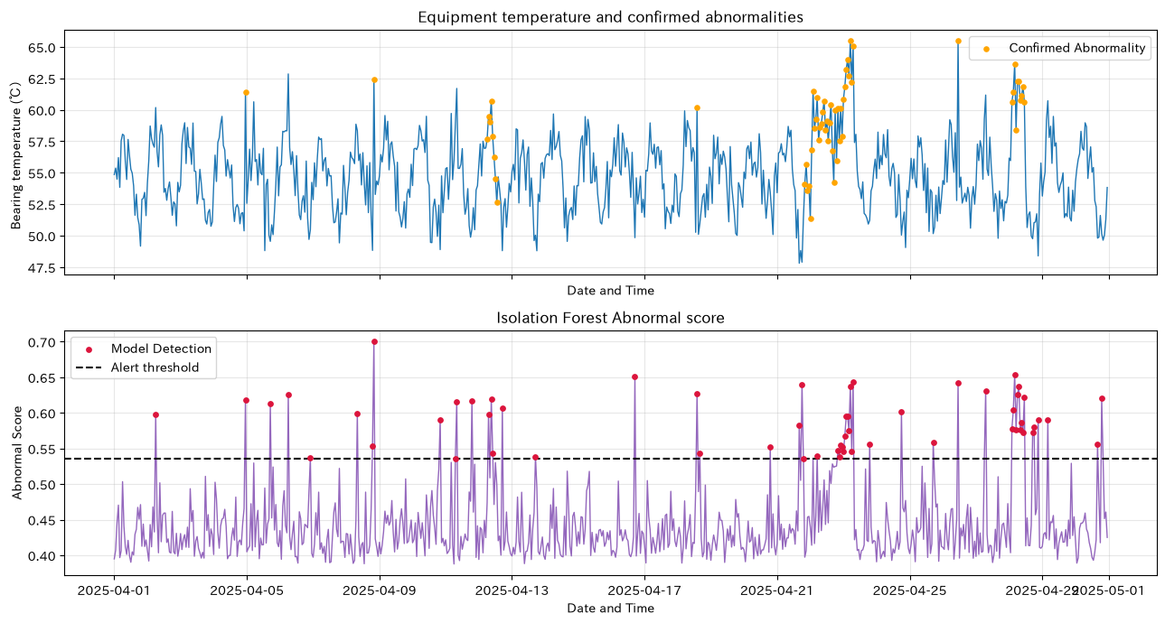

Reading the results

Sections with consecutive detection points have higher priority than single-shot noise and should be matched against maintenance records and production conditions. Contextual anomalies that are not visible by temperature also appear on the score side, so displaying multiple levels helps with decision-making.

No.080: Designing alerts that consider false positives and missed spots

Meaning in Practice

Even with high model accuracy, too many alerts can be ignored. Clearly indicate the man-hours per inspection item, the downtime loss if overlooked, and the number of cases that can be handled, setting thresholds for each task.

Approach to Analysis and Modeling

If we $FP$ false positives, $FN$ misses, and set the costs of each as $C_{FP},C_{FN}$, then the evaluation cost is

$$Cost = C_{FP}FP + C_{FN}FN$$

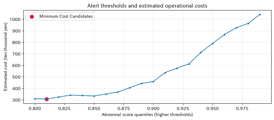
That’s right. Here, assuming 5,000 yen for one false positive and 200,000 yen for one missed hour, the cost is compared by score quantile. Furthermore, single detection is called “Caution,” and if there are two or more times within the 3-hour window, alert fatigue is reduced.

Check with Python

rows = []
for q in np.arange(0.80, 0.991, 0.01):
    threshold = df["score_iso"].quantile(q)
    pred = (df["score_iso"] >= threshold).astype(int)
    tn, fp, fn, tp = confusion_matrix(df["is_anomaly"], pred).ravel()
    rows.append({
        "quantile": q, "threshold": threshold, "TP": tp, "FP": fp, "FN": fn,
        "Compatibility rate": precision_score(df["is_anomaly"], pred, zero_division=0),
        "recall rate": recall_score(df["is_anomaly"], pred),
        "estimated_cost_ten_thousand_yen": (fp * 5_000 + fn * 200_000) / 10_000,
    })
cost_table = pd.DataFrame(rows)
best = cost_table.loc[cost_table["estimated_cost_ten_thousand_yen"].idxmin()]
display(cost_table.nsmallest(5, "estimated_cost_ten_thousand_yen").round(3))

best_pred = (df["score_iso"] >= best["threshold"]).astype(int)
recent_hits = best_pred.rolling(3, min_periods=1).sum()
df["alert_level"] = np.select(
    [recent_hits >= 2, best_pred == 1], ["warning", "Note"], default="normal"
)
print(f"Candidate for Employment: quantile={best['quantile']:.2f}, estimated_cost={best['estimated_cost_ten_thousand_yen']:.1f}ten_thousand_yen")
display(df["alert_level"].value_counts().rename("hours").to_frame())

fig, ax = plt.subplots(figsize=(9, 4))
ax.plot(cost_table["quantile"], cost_table["estimated_cost_ten_thousand_yen"], marker="o", markersize=3)
ax.scatter(best["quantile"], best["estimated_cost_ten_thousand_yen"], color="crimson", s=70, label="Minimum Cost Candidates")
ax.set_title("Alert thresholds and estimated operational costs")
ax.set_xlabel("Abnormal score quantiles (higher thresholds)")
ax.set_ylabel("Estimated cost (ten thousand yen)")
ax.grid(True, alpha=0.3)
ax.legend()
fig.tight_layout()
plt.show()

	quantile	threshold	TP	FP	FN	Compatibility rate	recall rate	estimated_cost_ten_thousand_yen
1	0.81	0.47	45	92	13	0.33	0.78	306.00
0	0.80	0.47	45	99	13	0.31	0.78	309.50
2	0.82	0.47	44	86	14	0.34	0.76	323.00
5	0.85	0.49	43	65	15	0.40	0.74	332.50
4	0.84	0.48	43	73	15	0.37	0.74	336.50

Candidate for recruitment: Quantile = 0.81, Estimated cost = 3,060,000 yen

	hours
alert_level
normal	565
warning	85
Note	70

Reading the results

If the missed value is set high, a threshold is chosen that allows for some false positives and prioritizes recall. However, since the amount is assumed, the equipment downtime, safety impact, and inspection man-hours are updated in agreement with the site. Only by deciding on continuous checks, cooldown times, and stepping according to equipment importance can alerts be implemented for the first time.

Practical Implications Seen Through Target Exercise

1. Defining abnormalities comes first, then selecting methods: The effective methods differ depending on point, context, set, and multivariate anomaly.
2. Don’t abandon simple statistical methods: Z-scores and IQRs are highly explainable and serve as benchmarks for model monitoring.
3. Include driving conditions in the feature: If load and product type are not considered, normal high-load operation may be falsely detected.
4. Don’t mistake scores for probabilities: Treat as rankings within the same model, and set thresholds based on the number of inspections and costs.
5. Visualization and response flows determine outcomes: Not only detects, but also leads to cause identification, recording, and relearning.

What is necessary for practical implementation

• Data quality management including sensor calibration, missing measurements, communication outages, and post-maintenance value changes
• A data platform linking equipment ID, variety, load, schedule, and maintenance history
• Defining false positive/missed costs by equipment criticality and failure mode
• Clearly state alert notification destinations, initial confirmation, escalation, and response deadlines
• A system to accumulate on-site feedback as a correct answer label
• Operational KPIs that regularly review data distribution, number of alerts, and post-detection results

In phased implementation, shadow operations are first conducted in one equipment and one failure mode, and after accumulating actual inspection results, notifications are implemented to reduce risk.

Conclusion

From No.071 to No.080, we covered everything from organizing anomaly types to statistical detection, unsupervised learning, multivariate evaluation, visualization, and cost-based alert design. Rather than choosing the best algorithm, it is important to combine easy-to-explain rules and multivariate models and operate them according to the on-site response capabilities.

Consultations for Corporations

At Surikou, we support you according to your challenges and data maturity, from organizing manufacturing data, PoC for equipment anomaly detection, integrating into existing maintenance workflows, to on-site training.

📩 Contact Us: surikobo.co.jp/contact
Please feel free to consult us first.