Feature Design to Strengthen Demand Forecasting in Manufacturing — 10 Exercises to Turn Order History into Decision Information

In this article, we design features from Only information that can truly be used at the time of prediction using the order history of a fictional parts manufacturer as the subject. The goal is to convert days of the week, holidays, past demand, and customer and product characteristics into usable forms for inventory, personnel, and production planning.

The subject is No.051〜No.060 of Chapter 6 of “100 Machine Learning Exercises.” We not only run the code but also verify the operational meaning of features, how to create them, how to read results, and operations to prevent data leaks.

[!NOTE] This material is a notebook previously used by Surikoubo (or personally by the representative, Kazuyama), and has been reconstructed, edited, and published with the company’s permission. All data listed is fictional and has no relation whatsoever to real companies, factories, or figures.

Introduction: Practical Challenges in Manufacturing Covered in This Article

At parts manufacturers, they forecast the order volume for the following week and decide on material arrangements, equipment slots, overtime, and outsourcing. However, raw order data alone cannot convey month-end concentration, holidays, order cycles per customer, or demand levels for each product to the model. This article focuses on the process of translating history into explanatory variables that can be used for prediction.

Common situations on site

• Extracting dates, customers, products, and quantities from ERP but directly entering them into the model
• Using the average over the entire period as a feature ensures accuracy only during verification
• Filling missing lags with zero and confusing days off with missing history
• The definition of features and their availability timing are individualized.

Why is this issue so difficult to judge?

Features cannot be evaluated solely with predictive accuracy. It is also important to determine whether it can be obtained at the time of plan finalization, whether it can be generated with the same definition in the future, and whether the field can explain the meaning. Especially in chronological sequences, even a slight mix of future achievements can cause verification values to become exaggerated.

Overview of Exercise covered this time

No.	Theme	Connection to Planning Operations
051	Date feature	Weekday Cycle, Month, and Quarter Cycle
052	Holidays & Business Days	Operating Days and Holiday Effects
053	rug	Recent and Weekday Demand
054	moving average	Standard Demand and Fluctuations
055	Customer Aggregation	Customer-specific order levels
056	Product-specific aggregation	Item-specific demand levels
057	ratio	Capacity Load and Composition Ratio
058	interaction	Combination of Conditions Effects
059	Target Encoding	Quantifying High Cardinality
060	Data Leak Prevention	Ensuring Realistic Reproduction of the Performance

Preparing the Python environment

numpy use pandas, matplotlib, and scikit-learn. Keep the random seed fixed, and keep the graph readable even after Markdown conversion.

import numpy as np
import pandas as pd
import matplotlib
import matplotlib.pyplot as plt
from sklearn.compose import ColumnTransformer
from sklearn.ensemble import RandomForestRegressor
from sklearn.metrics import mean_absolute_error
from sklearn.pipeline import Pipeline
from sklearn.preprocessing import OneHotEncoder

SEED = 42
rng = np.random.default_rng(SEED)
plt.rcParams["figure.figsize"] = (9, 4.5)
plt.rcParams["axes.unicode_minus"] = False

print("numpy:", np.__version__)
print("pandas:", pd.__version__)
print("matplotlib:", matplotlib.__version__)

numpy: 2.5.1
pandas: 3.0.3
matplotlib: 3.11.0

Creation of Fictional Data

From January 2024 to June 2025, we will create daily records for 8 customers × 5 products. The objective variable is the order quantity order_qty. It includes the day of the week, end of month, customer size, product popularity, promotions, and the impact of holidays. capacity_qty Standard capacity that can be assigned on that day. No external data is used.

dates = pd.date_range("2024-01-01", "2025-06-30", freq="D")
customers = [f"C{i:02d}" for i in range(1, 9)]
products = [f"P{i:02d}" for i in range(1, 6)]
idx = pd.MultiIndex.from_product([dates, customers, products], names=["date", "customer_id", "product_id"])
df = idx.to_frame(index=False)

customer_scale = {c: v for c, v in zip(customers, [0.75, 0.9, 1.05, 1.25, 1.5, 0.85, 1.15, 1.35])}
product_base = {p: v for p, v in zip(products, [18, 25, 34, 43, 55])}
product_capacity = {p: v for p, v in zip(products, [52, 58, 68, 78, 90])}
df["promotion"] = (rng.random(len(df)) < 0.045).astype(int)
df["unit_price"] = df["product_id"].map(dict(zip(products, [1280, 1650, 2100, 2480, 3150])))

# A fictional calendar modeled after Japanese holidays (does not depend on external calendars)
holiday_dates = pd.to_datetime([
    "2024-01-01", "2024-01-08", "2024-02-12", "2024-02-23", "2024-04-29",
    "2024-05-03", "2024-05-06", "2024-07-15", "2024-08-12", "2024-09-16",
    "2024-10-14", "2024-11-04", "2025-01-01", "2025-01-13", "2025-02-11",
    "2025-02-24", "2025-04-29", "2025-05-05", "2025-05-06"
])
weekday = df["date"].dt.dayofweek
is_holiday = df["date"].isin(holiday_dates)
business = ((weekday < 5) & ~is_holiday).astype(int)
month_end = (df["date"].dt.day >= 25).astype(int)
season = 1 + 0.10 * np.sin(2 * np.pi * (df["date"].dt.month - 1) / 12)
mu = (df["product_id"].map(product_base) * df["customer_id"].map(customer_scale)
      * season * (1 + 0.18 * month_end) * (1 + 0.28 * df["promotion"])
      * np.where(business == 1, 1.0, 0.16))
df["order_qty"] = rng.poisson(mu).astype(int)
df["capacity_qty"] = df["product_id"].map(product_capacity)
df["revenue"] = df["order_qty"] * df["unit_price"]

print("shape:", df.shape)
display(df.head())

Shape: (21880, 8)

	date	customer_id	product_id	promotion	unit_price	order_qty	capacity_qty	revenue
0	2024-01-01	C01	P01	0	1280	4	52	5120
1	2024-01-01	C01	P02	0	1650	4	58	6600
2	2024-01-01	C01	P03	0	2100	3	68	6300
3	2024-01-01	C01	P04	0	2480	7	78	17360
4	2024-01-01	C01	P05	0	3150	7	90	22050

No.051: Creating Days of the Week, Month, and Quarter from Dates

Meaning in Practice

Dates are not just identifiers; they represent the production and shipping cycles. Weekdays are for dispatch and closing, monthly is seasonal demand, and quarterly is for budgeting and inventory cycles to the model.

Approach to Analysis and Modeling

From date $t$ to day of the week, $d(t)$ month $m(t)$, quarterly $q(t)=\lfloor(m(t)-1)/3\rfloor+1$. Because numbers have room for mislearning between large and small relationships, some models treat them as categories.

Check with Python

df["day_of_week"] = df["date"].dt.dayofweek
df["day_name"] = df["date"].dt.day_name()
df["month"] = df["date"].dt.month
df["quarter"] = df["date"].dt.quarter
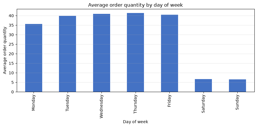
calendar_summary = df.groupby("day_name", observed=True)["order_qty"].mean().reindex(
    ["Monday", "Tuesday", "Wednesday", "Thursday", "Friday", "Saturday", "Sunday"])
display(calendar_summary.rename("mean_order_qty").round(2).to_frame())
calendar_summary.plot(kind="bar", color="#4472C4")
plt.title("Average order quantity by day of week")
plt.xlabel("Day of week"); plt.ylabel("Average order quantity"); plt.grid(axis="y", alpha=.3); plt.tight_layout(); plt.show()

	mean_order_qty
day_name
Monday	35.70
Tuesday	39.81
Wednesday	40.99
Thursday	41.38
Friday	40.45
Saturday	6.64
Sunday	6.51

Reading the results

The difference in standards between weekdays and weekends is clear. Based on the day of the week feature, the model can distinguish between production just before holidays and shipping loads at the start of the week. However, do not definitively attribute the cause to the day of the week; instead, confirm the closing time and correspondence with delivery services on-site.

No.052: Create Holiday and Business Day Flags

Meaning in Practice

The calendar days do not match the actual number of days available. Specifying holidays allows you to separate decreased demand and equipment outages from fluctuations on regular days.

Approach to Analysis and Modeling

If you $H_t$ belonging to a holiday gathering and $W_t$ a weekend, the business day flag is $B_t=1[(H_t=0)\land(W_t=0)]$. During production, company calendars, temporary operations, and customer-specific holidays are also managed.

Check with Python

df["is_holiday"] = df["date"].isin(holiday_dates).astype(int)
df["is_business_day"] = ((df["day_of_week"] < 5) & (df["is_holiday"] == 0)).astype(int)
business_summary = df.groupby("is_business_day")["order_qty"].agg(["mean", "median", "count"])
business_summary.index = ["non-business", "business"]
display(business_summary.round(2))
business_summary["mean"].plot(kind="bar", color=["#A5A5A5", "#70AD47"])
plt.title("Orders on business and non-business days")
plt.xlabel("Calendar class"); plt.ylabel("Average order quantity"); plt.grid(axis="y", alpha=.3); plt.tight_layout(); plt.show()

	mean	median	count
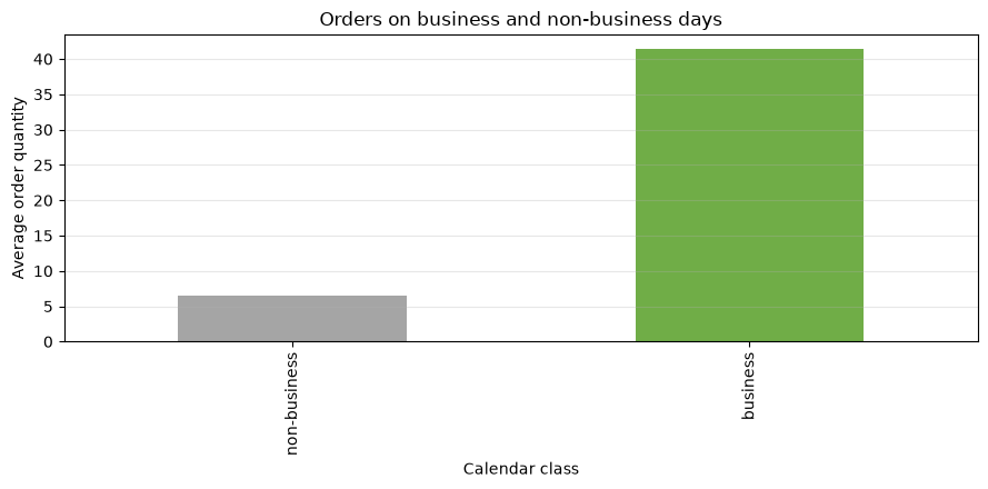
non-business	6.57	6.0	7000
business	41.35	38.0	14880

Reading the results

The average order volume on non-business days has dropped significantly compared to business days. The business day flag is a prerequisite for material and personnel planning. Whether to use the order date or desired delivery date is defined according to the target variable.

No.053: Creating Rug Features

Meaning in Practice

Orders received yesterday and the same week last week are strong clues to short-term planning. We capture sudden fluctuations and replicate the exemplary rules of purchasing and production personnel.

Approach to Analysis and Modeling

Create $L_{t,k}=y_{t-k}$ for each series. Here, customers × refer to 1 day before and 7 days before each product. Conducting shift first is key to preventing the day’s performance from being mixed in.

Check with Python

df = df.sort_values(["customer_id", "product_id", "date"]).copy()
series_keys = ["customer_id", "product_id"]
df["lag_1"] = df.groupby(series_keys)["order_qty"].shift(1)
df["lag_7"] = df.groupby(series_keys)["order_qty"].shift(7)
sample = df.query("customer_id == 'C05' and product_id == 'P05'").tail(12)
display(sample[["date", "order_qty", "lag_1", "lag_7"]])
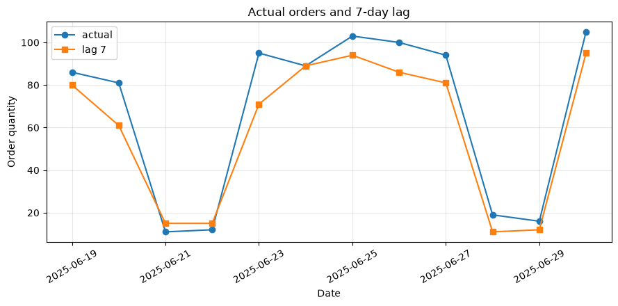
plt.plot(sample["date"], sample["order_qty"], marker="o", label="actual")
plt.plot(sample["date"], sample["lag_7"], marker="s", label="lag 7")
plt.title("Actual orders and 7-day lag"); plt.xlabel("Date"); plt.ylabel("Order quantity")
plt.grid(alpha=.3); plt.legend(); plt.xticks(rotation=30); plt.tight_layout(); plt.show()

	date	order_qty	lag_1	lag_7
21424	2025-06-19	86	94.0	80.0
21464	2025-06-20	81	86.0	61.0
21504	2025-06-21	11	81.0	15.0
21544	2025-06-22	12	11.0	15.0
21584	2025-06-23	95	12.0	71.0
21624	2025-06-24	89	95.0	89.0
21664	2025-06-25	103	89.0	94.0
21704	2025-06-26	100	103.0	86.0
21744	2025-06-27	94	100.0	81.0
21784	2025-06-28	19	94.0	11.0
21824	2025-06-29	16	19.0	12.0
21864	2025-06-30	105	16.0	95.0

Reading the results

The value from 7 days ago follows the level on the same day of the week. Missing items indicate no history at the beginning of the series, so instead of mechanical zero completion, remove them from the learning target or use the “insufficient history” flag.

No.054: Creating Moving Average Features

Meaning in Practice

Orders on a single day fluctuate by chance. Moving averages stabilize baseline demand and support decisions regarding safety stock and capacity planning.

Approach to Analysis and Modeling

The average of the most recent $w$ days is $MA_{t,w}=\frac{1}{w}\sum_{i=1}^{w}y_{t-i}$. Since the day is not included, calculations are made in shift(1).rolling(w) order.

Check with Python

g = df.groupby(series_keys)["order_qty"]
df["rolling_mean_7"] = g.transform(lambda s: s.shift(1).rolling(7, min_periods=3).mean())
df["rolling_mean_28"] = g.transform(lambda s: s.shift(1).rolling(28, min_periods=7).mean())
sample = df.query("customer_id == 'C05' and product_id == 'P05'").tail(60)
plt.plot(sample["date"], sample["order_qty"], alpha=.45, label="actual")
plt.plot(sample["date"], sample["rolling_mean_7"], label="7-day mean")
plt.plot(sample["date"], sample["rolling_mean_28"], label="28-day mean")
plt.title("Short- and medium-term demand baselines"); plt.xlabel("Date"); plt.ylabel("Order quantity")
plt.grid(alpha=.3); plt.legend(); plt.xticks(rotation=30); plt.tight_layout(); plt.show()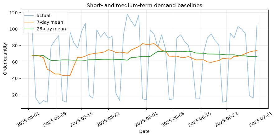

Reading the results

The 7-day average reacts quickly to recent changes, while the 28-day average remains stable. For short-term staff, the former is used; for monthly purchases, the latter is chosen—choosing the window width according to the lead time for decision-making.

No.055: Creating Customer-Specific Aggregated Features

Meaning in Practice

Order sizes and variability vary by customer. Historical averages and variance can be used to forecast the load of key customers and design forecast intervals.

Approach to Analysis and Modeling

For each customer, cumulative statistics prior to the forecast date are used. The average of the extended window is $\bar y_{c,t-1}$, and it is important not to lump the average over all periods.

Check with Python

customer_daily = df.groupby(["date", "customer_id"], as_index=False)["order_qty"].sum()
customer_daily = customer_daily.sort_values(["customer_id", "date"])
customer_daily["customer_past_mean"] = customer_daily.groupby("customer_id")["order_qty"].transform(
    lambda s: s.shift(1).expanding().mean())
customer_profile = customer_daily.groupby("customer_id").agg(
    latest_past_mean=("customer_past_mean", "last"), observed_std=("order_qty", "std"))
display(customer_profile.round(2).sort_values("latest_past_mean", ascending=False))
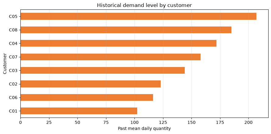
customer_profile["latest_past_mean"].sort_values().plot(kind="barh", color="#ED7D31")
plt.title("Historical demand level by customer"); plt.xlabel("Past mean daily quantity"); plt.ylabel("Customer")
plt.grid(axis="x", alpha=.3); plt.tight_layout(); plt.show()

	latest_past_mean	observed_std
customer_id
C05	206.99	115.22
C08	184.89	102.48
C04	171.93	95.56
C07	158.00	87.48
C03	144.15	79.93
C02	122.89	68.19
C06	116.22	64.75
C01	102.44	57.00

Reading the results

We were able to identify high-level customers such as C05. By combining not only the average but also the standard deviation and the number of days since the final order, you can distinguish between securing capability and following up on sales.

No.056: Creating Product-Specific Aggregated Features

Meaning in Practice

The scale and volatility of demand for each product provide basic information for material requirements and planning plans. Simply quantifying the item code cannot directly represent this level difference.

Approach to Analysis and Modeling

Create daily demand by product and calculate cumulative averages for only past periods. Since new products have little history, we are considering reducing operations to the average product line.

Check with Python

product_daily = df.groupby(["date", "product_id"], as_index=False)["order_qty"].sum()
product_daily = product_daily.sort_values(["product_id", "date"])
product_daily["product_past_mean"] = product_daily.groupby("product_id")["order_qty"].transform(
    lambda s: s.shift(1).expanding().mean())
product_profile = product_daily.groupby("product_id").agg(
    latest_past_mean=("product_past_mean", "last"), max_daily=("order_qty", "max"))
display(product_profile.round(2))
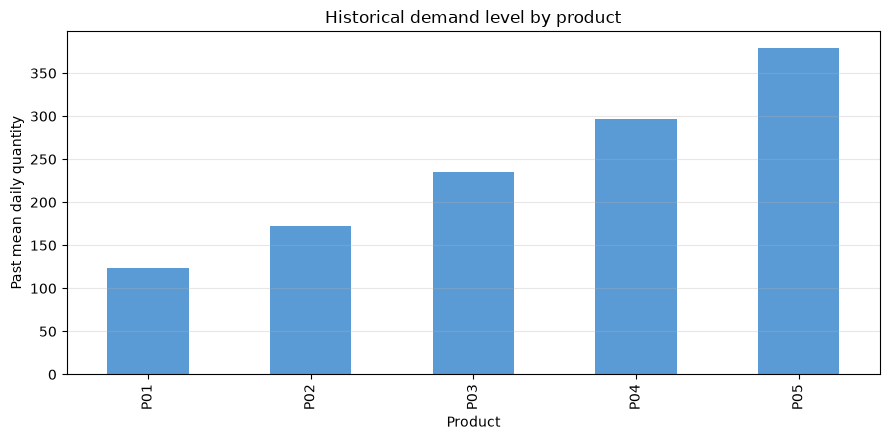
product_profile["latest_past_mean"].plot(kind="bar", color="#5B9BD5")
plt.title("Historical demand level by product"); plt.xlabel("Product"); plt.ylabel("Past mean daily quantity")
plt.grid(axis="y", alpha=.3); plt.tight_layout(); plt.show()

	latest_past_mean	max_daily
product_id
P01	124.02	228
P02	172.20	318
P03	235.02	428
P04	296.70	555
P05	379.57	672

Reading the results

P05 has a higher demand level than P01. By characterizing these differences, the model can have baseline lines for each item. However, it is necessary to reconsider whether to use old history with the same weight even after discontinuation or price revision.

No.057: Creating Ratio Features

Meaning in Practice

You cannot judge whether the quantity is heavy relative to its capability based on absolute quantity. Load rates and customer composition ratios can be compared using common metrics to show congestion and importance.

Approach to Analysis and Modeling

Let the load rate be $r_t=y_t/c_t$. If the denominator is zero or undetermined, it is treated as a missing value and it is important not to forcibly divide it with minute values. Here, for forecasting, we divide the 7-day average demand by capacity.

Check with Python

df["demand_capacity_ratio"] = df["rolling_mean_7"].div(df["capacity_qty"].replace(0, np.nan))
ratio_summary = df.groupby("product_id")["demand_capacity_ratio"].agg(["mean", "median", "max"])
display(ratio_summary.round(3))
plot_data = df.dropna(subset=["demand_capacity_ratio"]).sample(2500, random_state=SEED)
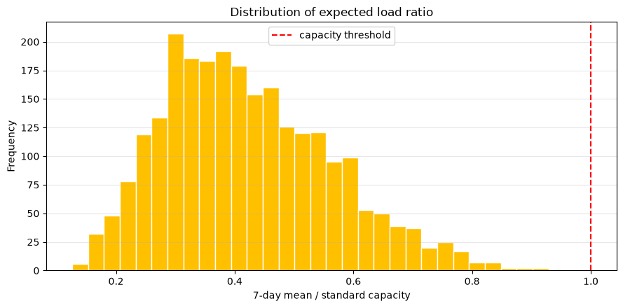
plt.hist(plot_data["demand_capacity_ratio"], bins=30, color="#FFC000", edgecolor="white")
plt.axvline(1.0, color="red", linestyle="--", label="capacity threshold")
plt.title("Distribution of expected load ratio"); plt.xlabel("7-day mean / standard capacity"); plt.ylabel("Frequency")
plt.grid(axis="y", alpha=.3); plt.legend(); plt.tight_layout(); plt.show()

	mean	median	max
product_id
P01	0.298	0.291	0.585
P02	0.371	0.362	0.687
P03	0.433	0.422	0.845
P04	0.476	0.462	0.842
P05	0.528	0.514	0.941

Reading the results

Above 1.0 is expected to exceed standard capacity. By viewing the frequency of high workloads by item, you can narrow down the options for overtime, outsourcing, and moving up the workload. We will always manage the frequency of ability updates and unit alignment.

No.058: Creating Interaction Features

Meaning in Practice

The promotional effect is not uniform and may intensify at the end of the month or with certain products. It clearly indicates “combination conditions” that are difficult to express with a single feature number.

Approach to Analysis and Modeling

Add the product $x_1x_2$ of the 2-variable $x_1,x_2$. Here, you create promotion × month_end and business_day × lag_7 to represent the concentrated sales promotion and the demand from the previous week on the business day.

Check with Python

df["is_month_end"] = (df["date"].dt.day >= 25).astype(int)
df["promotion_month_end"] = df["promotion"] * df["is_month_end"]
df["business_lag_7"] = df["is_business_day"] * df["lag_7"]
interaction_summary = df.groupby(["promotion", "is_month_end"])["order_qty"].mean().unstack()
interaction_summary.columns = ["not_month_end", "month_end"]
display(interaction_summary.round(2))
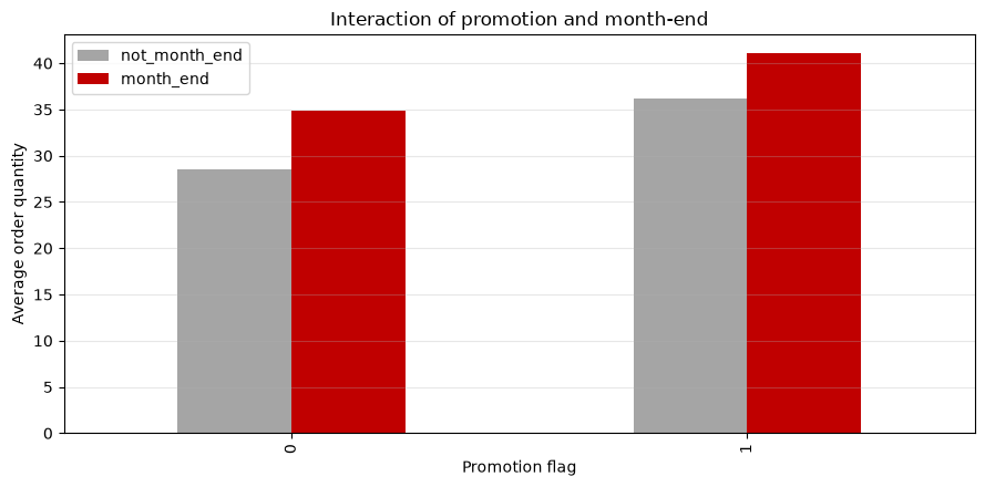
interaction_summary.plot(kind="bar", color=["#A5A5A5", "#C00000"])
plt.title("Interaction of promotion and month-end"); plt.xlabel("Promotion flag"); plt.ylabel("Average order quantity")
plt.grid(axis="y", alpha=.3); plt.legend(); plt.tight_layout(); plt.show()

	not_month_end	month_end
promotion
0	28.57	34.89
1	36.13	41.03

Reading the results

The combination of promotional and month-end promotions results in the largest average quantity. Interaction can pass hypotheses about policy effects to the model, but if you increase the number of candidates without limit, overlearning can occur, so focus on field hypotheses and testing.

No.059: Using Target Encoding

Meaning in Practice

If there are many categories such as customers, products, or facilities, One-Hot Encoding increases the number of columns. You can summarize categories into a single column at the level of past objective variables.

Approach to Analysis and Modeling

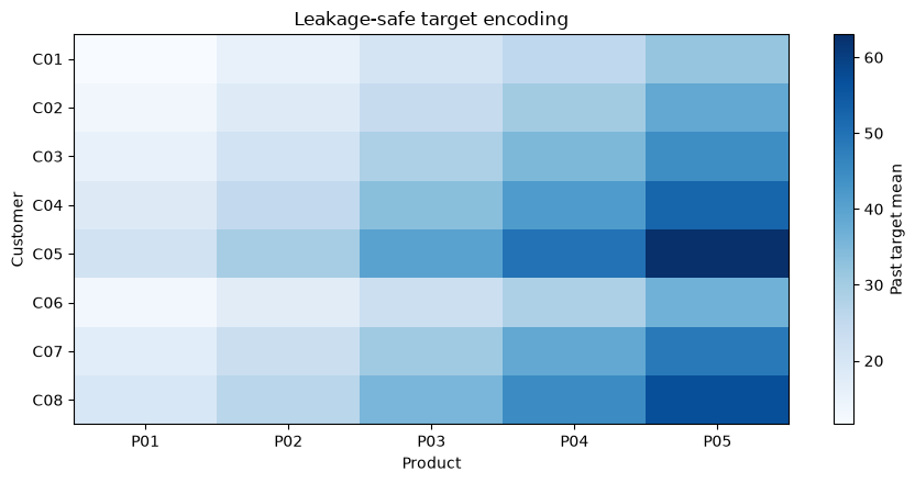
Replace the value of category $c$ with the smoothing average $TE_c=(n_c\bar y_c+m\mu)/(n_c+m)$. Here, only before each row, the cumulative sum and number of products × customers and the overall pre-average are calculated. $m$ is the strength of a minority category that brings it closer to the overall average.

Check with Python

df = df.sort_values("date").copy()
cat_key = df["customer_id"] + "_" + df["product_id"]
past_sum = df.groupby(cat_key)["order_qty"].cumsum() - df["order_qty"]
past_count = df.groupby(cat_key).cumcount()
global_past_sum = df["order_qty"].cumsum() - df["order_qty"]
global_past_count = np.arange(len(df))
global_prior = global_past_sum.div(pd.Series(global_past_count, index=df.index).replace(0, np.nan))
smoothing = 30
df["target_encoding"] = (past_sum + smoothing * global_prior) / (past_count + smoothing)
te_summary = df.groupby(["customer_id", "product_id"])["target_encoding"].last().unstack()
display(te_summary.round(2))
plt.imshow(te_summary, aspect="auto", cmap="Blues")
plt.colorbar(label="Past target mean"); plt.xticks(range(len(te_summary.columns)), te_summary.columns)
plt.yticks(range(len(te_summary.index)), te_summary.index)
plt.title("Leakage-safe target encoding"); plt.xlabel("Product"); plt.ylabel("Customer")
plt.grid(False); plt.tight_layout(); plt.show()

product_id	P01	P02	P03	P04	P05
customer_id
C01	11.62	15.37	20.65	25.38	31.95
C02	13.37	17.92	24.23	30.20	38.64
C03	15.59	21.16	28.28	34.99	44.49
C04	18.31	25.00	33.46	41.62	52.44
C05	21.55	29.67	39.95	49.89	63.02
C06	12.86	17.41	22.76	28.41	36.60
C07	17.20	22.92	30.61	38.53	48.38
C08	19.65	26.36	35.42	44.82	56.87

Reading the results

The demand level for customer× products can be represented in a single column. New categories fall back to the overall average. If you randomly divide training and validation and then calculate the overall average, it will leak, so calculate in chronological order or outside the fold.

No.060: Preventing Data Leaks

Meaning in Practice

Even if verification accuracy is high, if unknown information is used at the time of production, it cannot be used for planning. Leak prevention is a quality requirement that predates algorithm selection.

Approach to Analysis and Modeling

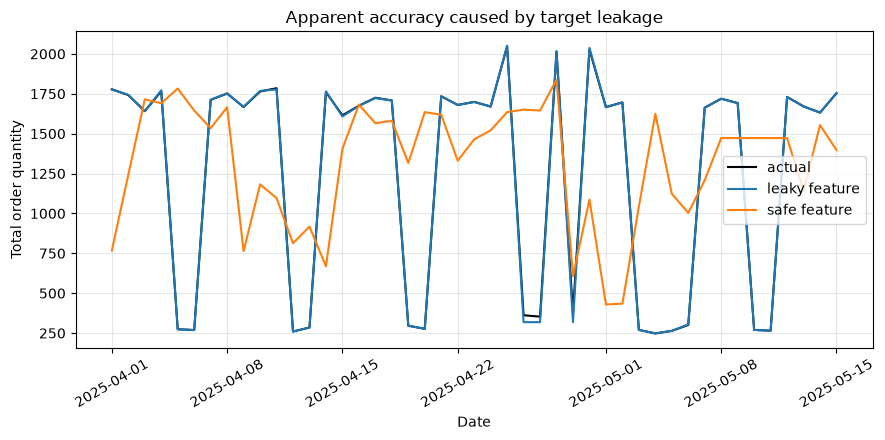
It learns at point $T$ and validates beyond $T$. Dangerous feature leaky_target is the objective variable left on the day due to a combination mismatch, while safe safe_roll is the moving average after the one-day shift. We confirm the overvaluation based on the MAE difference between the two.

Check with Python

daily = df.groupby("date", as_index=False)["order_qty"].sum().sort_values("date")
daily["leaky_target"] = daily["order_qty"]  # Unknown at the time of prediction. Typical leaks for explanation
daily["safe_roll"] = daily["order_qty"].shift(1).rolling(7, min_periods=7).mean()
daily = daily.dropna().copy()
cutoff = pd.Timestamp("2025-04-01")
train = daily[daily["date"] < cutoff]
test = daily[daily["date"] >= cutoff]

results = []
predictions = {}
for feature in ["leaky_target", "safe_roll"]:
    model = RandomForestRegressor(n_estimators=150, min_samples_leaf=4, random_state=SEED, n_jobs=1)
    model.fit(train[[feature]], train["order_qty"])
    pred = model.predict(test[[feature]])
    predictions[feature] = pred
    results.append({"feature": feature, "MAE": mean_absolute_error(test["order_qty"], pred)})
display(pd.DataFrame(results).set_index("feature").round(2))
view = test.iloc[:45]
plt.plot(view["date"], view["order_qty"], label="actual", color="black")
plt.plot(view["date"], predictions["leaky_target"][:45], label="leaky feature")
plt.plot(view["date"], predictions["safe_roll"][:45], label="safe feature")
plt.title("Apparent accuracy caused by target leakage"); plt.xlabel("Date"); plt.ylabel("Total order quantity")
plt.grid(alpha=.3); plt.legend(); plt.xticks(rotation=30); plt.tight_layout(); plt.show()

	MAE
feature
leaky_target	3.34
safe_roll	613.13

Reading the results

Features, which retain the objective variable itself, unnaturally show good MAE, but it cannot be created during prediction. For each feature, it is necessary to record the “occurrence time, finalization time, and acquisition time,” verify it using time series segmentation, and use the same generation process for training and inference.

Practical Implications Seen Through Target Exercise

Feature design is not about increasing data, but about projecting the timeline and decision-making of the business into the model. Calendar features represent the operating cycle, lag and moving averages represent demand memory, customer and product aggregation represent structural differences, ratios represent constraints, and interactions represent business hypotheses.

The priority for improving accuracy is to first maintain the available timeline, then align decision lead times and granularity, and finally increase the number of features. Acceptance decisions are made not only based on verification values but also on business KPIs such as out-of-stock, overtime, inventory, and the number of plan changes.

What is necessary for practical implementation

1. Prediction Specifications: Define the target, granularity, forecast date, forecast period, and plan finalization time
2. Data time management: Manage the occurrence, confirmation, and acquisition times for each item, as well as correction rules.
3. feature ledger: Definition, Units, Window Width, Defect Processing, Leaving Responsible Persons
4. reproducible processing: Use the same code for learning and inference to save historical snapshots
5. Timeline Verification: Evaluate MAE and operational KPIs across multiple periods, including busy and holiday seasons.
6. Monitoring and Updates: Monitor distribution changes due to new products, customer composition, capabilities, and calendar changes

Conclusion

No.051–060 convert raw dates and order histories into meaningful features for manufacturing planning. The most important point is to create all features with information prior to the prediction point. If you want to start small, start with business days, 7-day lag, 7-day moving averages, and historical averages by customer and product, and verify their effectiveness through time series verification.

Consultations for Corporations

In demand forecasting and inventory and production planning, data definition, features, validation, and on-site operations connections determine outcomes more than the model itself. At Suri Kobo, we support you with everything from problem organization, data diagnosis, PoC, business implementation, to corporate training, tailored to your data and decision-making process.

📩 Contact Us: surikobo.co.jp/contact Please feel free to consult us first.