Connecting Manufacturing Demand Forecasting to Order Decisions: 10 Time Series Exercises (No.061–No.070)

This practical notebook connects daily order and shipment records not just as line graphs but to Decision-making on production, inventory, and ordering. Using daily demand for the hypothetical industrial pump component “PX-100,” we handle everything in an integrated process: aggregation, trend and seasonality identification, forecasting models, time series verification, error analysis, and inventory simulation.

[!NOTE] This material is a notebook previously used by Surikoubo (or personally by the representative, Kazuyama), and has been reconstructed, edited, and published with the company’s permission.
All data listed is fictional and has no relation whatsoever to real companies, factories, or figures.

Introduction: Practical Challenges in Manufacturing Covered in This Article

In manufacturing, demand forecasts are linked to raw material orders, personnel allocation, production order, and finished goods inventory. Overforecasting leads to backlog inventory and cash tiebreakers, while underforecasting leads to stockouts, express shipping, and delivery delays. The purpose of this article is not only to “create highly accurate models,” but also to create a situation where the person in charge can determine the order volume for the following week in an explainable way, including the uncertainty of forecasts.

Common situations on site

• They only look at monthly totals and cannot grasp the impact of weekday differences or holidays.
• Although high accuracy was achieved through random splitting, it was not reproduced in actual operation.
• The average error is small, but it can be significantly off during important periods such as promotions and holidays
• Although forecasts were made, there were no rules to convert them into safety stock or ordering points.

Why is this issue so difficult to judge?

The time series overlaps with trends, cyclicality, and unexpected factors. Also, if you incorporate information you cannot know at the time of future prediction into features, data leaks only improve apparent accuracy. Furthermore, even with the same forecast error, out-of-stock and surplus business losses are asymmetrical. Therefore, chronological verification and evaluation based on operational costs are essential.

Overview of Exercise covered this time

No.	Theme	Connecting to decision-making
061	Daily Sales Visualization	Grasping fluctuation and abnormal periods
062	Weekly and monthly aggregation	Ability and Purchasing Plan Granularity Selection
063	moving average	Separation of Tone and Short-Term Noise
064	Seasonal Trends by Day of the Week and Month	Regular pre-weaving of mountain valleys
065	Lug Feature	Demand forecasting using recent performance
066	Regression Model	Forecasting that integrates multiple factors
067	Timeline Verification	Performance Evaluation Close to Production
068	Visualization of Prediction Errors	Understanding Biases and Variation
069	Analysis of the Missed Period	Identification of Improvement Targets and Exceptions
070	Connecting to Inventory and Order Planning	Balancing service standards and inventory costs

Preparing the Python environment

Handle data with pandas and numpy, visualize it with matplotlib, and build and evaluate models with scikit-learn. Random number seeds are fixed to 42. To avoid garbled characters caused by the execution environment, graphs are presented in English, and reading is explained in detail in the main text.

import warnings
warnings.filterwarnings("ignore", category=FutureWarning)

import numpy as np
import pandas as pd
import matplotlib.pyplot as plt
from sklearn.ensemble import RandomForestRegressor
from sklearn.linear_model import LinearRegression
from sklearn.metrics import mean_absolute_error, mean_squared_error
from sklearn.model_selection import TimeSeriesSplit

SEED = 42
rng = np.random.default_rng(SEED)
pd.set_option("display.max_columns", 20)
plt.rcParams["figure.figsize"] = (11, 4)
print("Libraries loaded. Random seed:", SEED)

Libraries loaded. Random seed: 42

Creation of Fictional Data

Generates daily data for two years starting from January 2024. The objective variable is the customer requested quantity demand_units the amount is sales_yen. Demand is expected to include moderate growth, weekday effects, monthly seasonality, promotional effects, a rush before the end of the year, summer holidays, and temporary supply constraints in April 2025.

Conceptually, daily demand $y_t$ is created as the next additive model.

$$y_t = T_t + W_t + S_t + 18P_t + E_t + \varepsilon_t, \qquad \varepsilon_t \sim \mathcal{N}(0, 5^2)$$

$T_t$ is the trend, $W_t$ is the day-of-the-week effect, $S_t$ is the monthly effect, $P_t$ is the promotional flag, and $E_t$ is the temporary factor. In practice, it is important to note that treating shipment performance without including backlogs or lost orders as “demand” underestimates the potential demand during supply constraint periods.

dates = pd.date_range("2024-01-01", periods=730, freq="D")
n = len(dates)
weekday_effect = np.array([8, 10, 9, 7, 4, -16, -20])
month_effect = {1: -5, 2: -2, 3: 8, 4: 3, 5: -1, 6: 5,
                7: 7, 8: -10, 9: 6, 10: 4, 11: 9, 12: 13}

df = pd.DataFrame({"date": dates})
df["weekday"] = df["date"].dt.dayofweek
df["month"] = df["date"].dt.month
df["promotion"] = ((df["date"].dt.day >= 10) & (df["date"].dt.day <= 12) &
                   (df["month"].isin([3, 6, 9, 11]))).astype(int)
trend = np.linspace(0, 16, n)
season = df["month"].map(month_effect).to_numpy()
special = np.zeros(n)
special[(df["date"].dt.month == 8) & (df["date"].dt.day.between(11, 16))] -= 30
special[(df["date"].dt.month == 12) & (df["date"].dt.day.between(16, 22))] += 22
supply_constraint = df["date"].between("2025-04-07", "2025-04-18")
special[supply_constraint] -= 24

latent = (72 + trend + weekday_effect[df["weekday"].to_numpy()] + season
          + 18 * df["promotion"].to_numpy() + special + rng.normal(0, 5, n))
df["demand_units"] = np.maximum(0, np.rint(latent)).astype(int)
df["unit_price_yen"] = 12500
df["sales_yen"] = df["demand_units"] * df["unit_price_yen"]
df["special_period"] = np.select(
    [supply_constraint,
     (df["date"].dt.month == 8) & (df["date"].dt.day.between(11, 16)),
     (df["date"].dt.month == 12) & (df["date"].dt.day.between(16, 22))],
    ["supply_constraint", "summer_shutdown", "year_end_rush"], default="normal")

print(f"Period: {df['date'].min().date()} to {df['date'].max().date()} / {len(df):,} days")
display(df.head())
display(df[["demand_units", "sales_yen"]].describe().round(1))

Period: 2024-01-01 to 2025-12-30 / 730 days

	date	weekday	month	promotion	demand_units	unit_price_yen	sales_yen	special_period
0	2024-01-01	0	1	0	77	12500	962500	normal
1	2024-01-02	1	1	0	72	12500	900000	normal
2	2024-01-03	2	1	0	80	12500	1000000	normal
3	2024-01-04	3	1	0	79	12500	987500	normal
4	2024-01-05	4	1	0	61	12500	762500	normal

	demand_units	sales_yen
count	730.0	730.0
mean	83.3	1041061.6
std	17.7	221419.6
min	11.0	137500.0
25%	72.0	900000.0
50%	84.0	1050000.0
75%	95.0	1187500.0
max	136.0	1700000.0

No.061: Visualize daily sales

Meaning in Practice

Daily trends are a starting point for checking short-term fluctuations that disappear from aggregates, business calendars, and sudden troughs. In manufacturing sites, it is important to record not only sales amounts but also quantities to avoid confusing price revisions with changes in quantity.

Approach to Analysis and Modeling

First, minimize processing and draw the original line. Observe changes in defects, zeros, steps, and variances, and hypothesize “rules the model should learn” and “exceptions to manage individually.”

Check with Python

fig, ax = plt.subplots()
ax.plot(df["date"], df["demand_units"], color="steelblue", linewidth=0.9)
ax.set_title("Daily Demand for PX-100")
ax.set_xlabel("Date")
ax.set_ylabel("Demand (units/day)")
ax.grid(True, alpha=0.3)
plt.tight_layout()
plt.show()
print("Peak day:")
display(df.nlargest(3, "demand_units")[["date", "demand_units", "promotion", "special_period"]])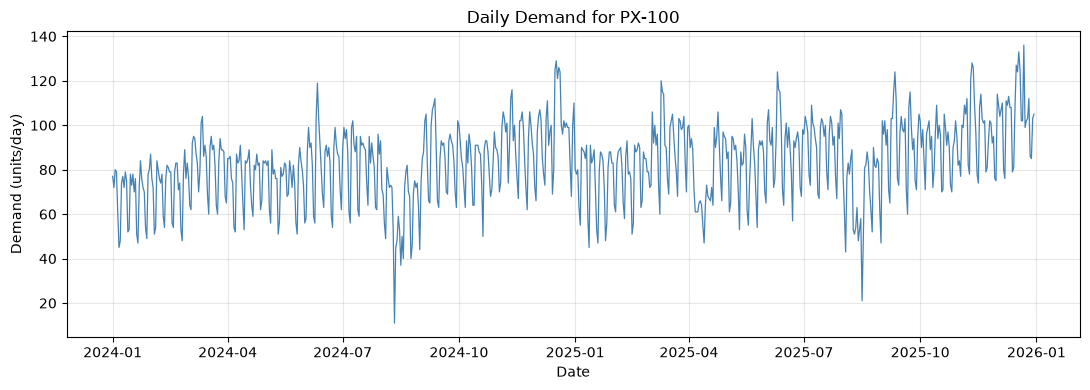

Peak day:

	date	demand_units	promotion	special_period
721	2025-12-22	136	0	year_end_rush
717	2025-12-18	133	0	year_end_rush
351	2024-12-17	129	0	year_end_rush

Reading the results

In addition to the regular weekend dip, there are peaks before promotions and year-end sales, and troughs during summer holidays and supply constraints. Therefore, it is inappropriate to determine daily production volume based solely on a simple full-period average. By cross-checking the background information of peak days in a table, you can distinguish whether the event is reproduced or transient.

No.062: Aggregating weekly and monthly sales

Meaning in Practice

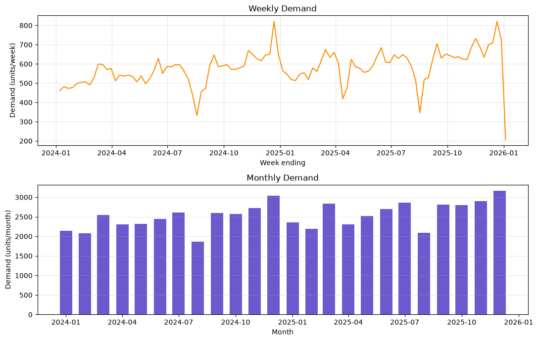
The level of granularity required varies depending on the decision: daily on-site staffing, weekly material ordering, and monthly S&OP and budgeting. By distinguishing between total quantity and average daily sales, you can prevent misreading due to differences in the number of days in a month.

Approach to Analysis and Modeling

The total period represents the required capacity, while the average period represents the intensity of demand. Weekly calculations start on Monday, and monthly calculations include both total and daily averages.

Check with Python

ts = df.set_index("date")
weekly = ts["demand_units"].resample("W-SUN").sum().rename("weekly_units")
monthly = ts["demand_units"].resample("MS").agg(["sum", "mean"])
monthly.columns = ["monthly_units", "avg_daily_units"]
display(monthly.tail(8).round(1))

fig, axes = plt.subplots(2, 1, figsize=(11, 7))
axes[0].plot(weekly.index, weekly, color="darkorange")
axes[0].set_title("Weekly Demand")
axes[0].set_xlabel("Week ending")
axes[0].set_ylabel("Demand (units/week)")
axes[0].grid(True, alpha=0.3)
axes[1].bar(monthly.index, monthly["monthly_units"], width=20, color="slateblue")
axes[1].set_title("Monthly Demand")
axes[1].set_xlabel("Month")
axes[1].set_ylabel("Demand (units/month)")
axes[1].grid(True, axis="y", alpha=0.3)
plt.tight_layout()
plt.show()

	monthly_units	avg_daily_units
date
2025-05-01	2519	81.3
2025-06-01	2702	90.1
2025-07-01	2864	92.4
2025-08-01	2091	67.5
2025-09-01	2810	93.7
2025-10-01	2802	90.4
2025-11-01	2901	96.7
2025-12-01	3161	105.4

Reading the results

While the week’s operating days and event effects remain, the monthly trend shows gradual growth and makes it easier to read the variations from month to month. Even when signing purchase contracts on a monthly basis, it is necessary to check not only the monthly total but also the weekly peak, and consider delivery frequency and storage capacity.

No.063: Seeing Trends with Moving Averages

Meaning in Practice

Frequently changing production plans in response to daily noise leads to more rescheduling and overtime. Moving averages are simple management indicators that smooth out short-term fluctuations and share a common pattern.

Approach to Analysis and Modeling

$k$ The daily moving average is as follows.

$$MA_t^{(k)}=\frac{1}{k}\sum_{i=0}^{k-1}y_{t-i}$$

The 7-day average smooths out the weekly cycle, while the 28-day average represents a medium-term trend. However, moving averages respond to changes later and are distinguished from the actual forecast value.

Check with Python

df["ma_7"] = df["demand_units"].rolling(7).mean()
df["ma_28"] = df["demand_units"].rolling(28).mean()
view = df.tail(240)
fig, ax = plt.subplots()
ax.plot(view["date"], view["demand_units"], color="lightgray", label="Daily", linewidth=0.8)
ax.plot(view["date"], view["ma_7"], label="7-day MA", linewidth=1.5)
ax.plot(view["date"], view["ma_28"], label="28-day MA", linewidth=2)
ax.set_title("Demand Trend with Moving Averages")
ax.set_xlabel("Date")
ax.set_ylabel("Demand (units/day)")
ax.grid(True, alpha=0.3)
ax.legend()
plt.tight_layout()
plt.show()
print("Latest moving averages:")
latest_ma = df[["date", "demand_units", "ma_7", "ma_28"]].tail(5).copy()
latest_ma[["ma_7", "ma_28"]] = latest_ma[["ma_7", "ma_28"]].round(1)
display(latest_ma)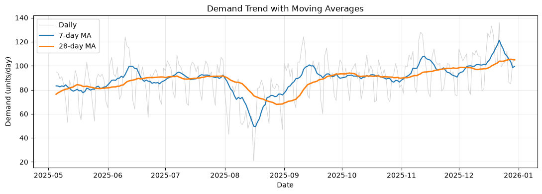

Latest moving averages:

	date	demand_units	ma_7	ma_28
725	2025-12-26	112	108.0	104.8
726	2025-12-27	86	105.7	105.1
727	2025-12-28	85	103.3	105.5
728	2025-12-29	103	98.6	105.1
729	2025-12-30	105	99.4	104.9

Reading the results

The 7-day average captures recent changes in supply and demand, while the 28-day average shows a stable trend. When the gap between the two widens, it signals a change in demand levels or a temporary event. Window widths are set according to procurement lead times and plan review cycles.

No.064: Viewing Seasonality by Day of the Week and Month

Meaning in Practice

Day-of-week differences relate to daily delivery and shipping schedules, while monthly differences relate to regular maintenance, budget fulfillment, and seasonal demand. By incorporating recurring patterns in advance, you can reduce the waste that is treated as an “anomaly” each time.

Approach to Analysis and Modeling

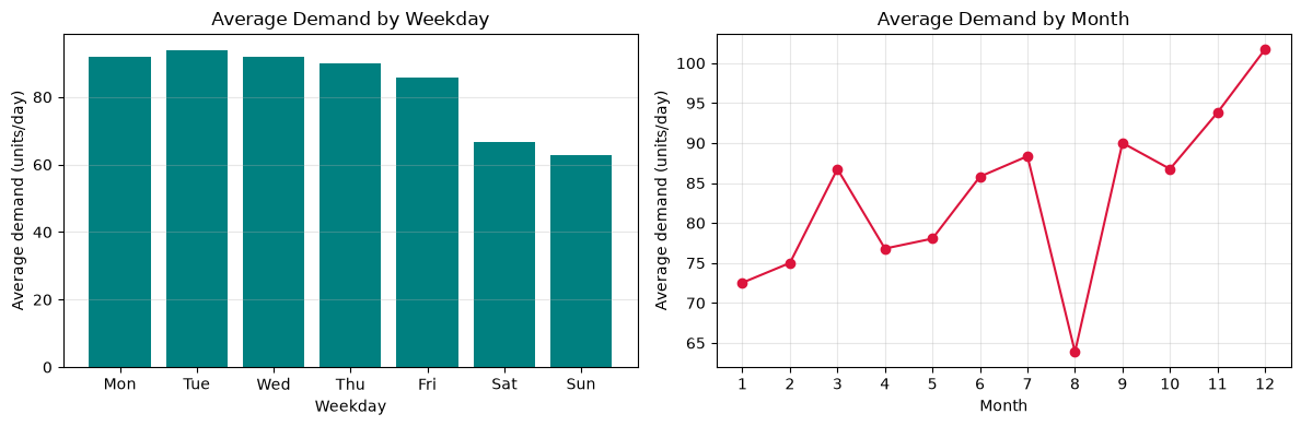
Divide the average values by day and month by the overall average to check the seasonal index. If the index is 1.10, the demand level is about 10% higher than average. Since the composition changes from year to year, we also check whether it remains stable over multiple years.

Check with Python

weekday_names = ["Mon", "Tue", "Wed", "Thu", "Fri", "Sat", "Sun"]
overall_mean = df["demand_units"].mean()
weekday_profile = df.groupby("weekday")["demand_units"].mean().reindex(range(7))
weekday_profile.index = weekday_names
month_profile = df.groupby("month")["demand_units"].mean().reindex(range(1, 13))
seasonality = pd.DataFrame({
    "weekday_avg": weekday_profile,
    "weekday_index": weekday_profile / overall_mean
})
display(seasonality.round(2))

fig, axes = plt.subplots(1, 2, figsize=(12, 4))
axes[0].bar(weekday_profile.index, weekday_profile.values, color="teal")
axes[0].set_title("Average Demand by Weekday")
axes[0].set_xlabel("Weekday")
axes[0].set_ylabel("Average demand (units/day)")
axes[0].grid(True, axis="y", alpha=0.3)
axes[1].plot(month_profile.index, month_profile.values, marker="o", color="crimson")
axes[1].set_title("Average Demand by Month")
axes[1].set_xlabel("Month")
axes[1].set_ylabel("Average demand (units/day)")
axes[1].set_xticks(range(1, 13))
axes[1].grid(True, alpha=0.3)
plt.tight_layout()
plt.show()

	weekday_avg	weekday_index
Mon	91.85	1.10
Tue	93.90	1.13
Wed	91.88	1.10
Thu	89.88	1.08
Fri	85.79	1.03
Sat	66.80	0.80
Sun	62.72	0.75

Reading the results

The pattern is clear: weekdays are high, especially in the first half of the week, while weekends are low. By month, you can check mountains before the end of the year and valleys in summer. This serves as a basis for not making the capacity plan uniform every day, but allocation according to regular patterns. However, since the average value is also influenced by the promotional structure, it cannot be definitively considered causation.

No.065: Forecasting Demand by Lug Feature

Meaning in Practice

Recent results and the same period last year are important information that staff refer to empirically. By using lag features, you can convert those decisions into reproducible calculations.

Approach to Analysis and Modeling

$L$ day lag is $x_t^{(L)}=y_{t-L}$. Here, we use the previous day, one week prior, two weeks prior, and four weeks prior. shift The key to preventing data leakage is to prevent mixing the day’s performance into the explanatory variables. First, we use the season-naive method as the baseline, which forecasts the results from one week earlier.

Check with Python

for lag in [1, 7, 14, 28]:
    df[f"lag_{lag}"] = df["demand_units"].shift(lag)
df["rolling_7_past"] = df["demand_units"].shift(1).rolling(7).mean()

lag_data = df.dropna(subset=["lag_1", "lag_7", "lag_14", "lag_28", "rolling_7_past"]).copy()
cutoff = pd.Timestamp("2025-09-01")
lag_test = lag_data[lag_data["date"] >= cutoff].copy()
lag_test["naive_pred"] = lag_test["lag_7"]
naive_mae = mean_absolute_error(lag_test["demand_units"], lag_test["naive_pred"])
naive_rmse = mean_squared_error(lag_test["demand_units"], lag_test["naive_pred"]) ** 0.5
print(f"Seasonal naive (lag 7) MAE: {naive_mae:.2f} units")
print(f"Seasonal naive (lag 7) RMSE: {naive_rmse:.2f} units")
display(lag_test[["date", "demand_units", "lag_1", "lag_7", "rolling_7_past", "naive_pred"]].head())

Seasonal naive (lag 7) MAE: 9.92 units
Seasonal naive (lag 7) RMSE: 12.72 units

	date	demand_units	lag_1	lag_7	rolling_7_past	naive_pred
609	2025-09-01	102	47.0	90.0	75.714286	90.0
610	2025-09-02	96	102.0	82.0	77.428571	82.0
611	2025-09-03	102	96.0	81.0	79.428571	81.0
612	2025-09-04	91	102.0	85.0	82.428571	85.0
613	2025-09-05	98	91.0	83.0	83.285714	83.0

Reading the results

Even just one week ago can reflect the day-of-the-week pattern, making it a strong benchmark model. Advanced models are only candidates for adoption if they improve within a practical range beyond this standard. If RMSE is greater than MAE, some major mismatches are pushing the valuation higher.

No.066: Time Series Prediction Using Regression Models

Meaning in Practice

Demand is determined not only by recent performance but also by multiple factors such as the day of the week, month, promotions, and trends. The regression model integrates these and quantifies next-day demand.

Approach to Analysis and Modeling

We compare random forests, which are easy to explain linear regression, as candidates for handling nonlinear relationships. Learning is fixed in the past, tests in the future, and evaluation metrics use MAE, which represents the average magnitude of error, and RMSE, which strongly punishes major deviations. The promotional schedule is assumed to be known at the time of prediction.

Check with Python

feature_cols = ["lag_1", "lag_7", "lag_14", "lag_28", "rolling_7_past",
                "weekday", "month", "promotion"]
model_data = lag_data.copy()
train = model_data[model_data["date"] < cutoff]
test = model_data[model_data["date"] >= cutoff].copy()
X_train, y_train = train[feature_cols], train["demand_units"]
X_test, y_test = test[feature_cols], test["demand_units"]

models = {
    "LinearRegression": LinearRegression(),
    "RandomForest": RandomForestRegressor(
        n_estimators=250, max_depth=8, min_samples_leaf=4,
        random_state=SEED, n_jobs=-1
    ),
}
rows = []
for name, model in models.items():
    model.fit(X_train, y_train)
    pred = model.predict(X_test)
    rows.append({"model": name,
                 "MAE": mean_absolute_error(y_test, pred),
                 "RMSE": mean_squared_error(y_test, pred) ** 0.5})
    test[f"pred_{name}"] = pred
comparison = pd.DataFrame(rows).set_index("model")
comparison.loc["SeasonalNaive"] = [naive_mae, naive_rmse]
display(comparison.sort_values("MAE").round(2))

best_name = comparison[comparison.index != "SeasonalNaive"]["MAE"].idxmin()
best_model = models[best_name]
test["prediction"] = test[f"pred_{best_name}"]
print("Selected regression model:", best_name)

	MAE	RMSE
model
RandomForest	6.17	8.29
LinearRegression	6.96	8.78
SeasonalNaive	9.92	12.72

Selected regression model: RandomForest

Reading the results

When comparing models, always check the extent of improvement compared to the seasonal naive method. If a complex model is only slightly better, there is room to choose linear models that include explainability, maintainability, and retraining effort. In this notebook, we use the regression model with the smaller test MAE for subsequent analysis.

No.067: Learning How to Verify Time Series Data

Meaning in Practice

A single test period may have coincided with a specific season. By verifying multiple past points in time and learning only from data up to that point and predicting what happens next, we estimate performance fluctuations during operation.

Approach to Analysis and Modeling

TimeSeriesSplit is a walk-forward validation that gradually extends the learning period. Unlike random splitting, it prevents information from mixing into the past. Not only the average for each fold, but also the worst-case fold is used for capacity and safety stock design.

Check with Python

tscv = TimeSeriesSplit(n_splits=5, test_size=60)
cv_rows = []
X_all, y_all = model_data[feature_cols], model_data["demand_units"]
for fold, (tr_idx, va_idx) in enumerate(tscv.split(X_all), start=1):
    fold_model = RandomForestRegressor(
        n_estimators=180, max_depth=8, min_samples_leaf=4,
        random_state=SEED, n_jobs=-1
    )
    fold_model.fit(X_all.iloc[tr_idx], y_all.iloc[tr_idx])
    fold_pred = fold_model.predict(X_all.iloc[va_idx])
    cv_rows.append({
        "fold": fold,
        "train_end": model_data.iloc[tr_idx[-1]]["date"].date(),
        "valid_start": model_data.iloc[va_idx[0]]["date"].date(),
        "valid_end": model_data.iloc[va_idx[-1]]["date"].date(),
        "MAE": mean_absolute_error(y_all.iloc[va_idx], fold_pred),
        "RMSE": mean_squared_error(y_all.iloc[va_idx], fold_pred) ** 0.5,
    })
cv_results = pd.DataFrame(cv_rows)
display(cv_results.round(2))
print(f"CV MAE mean: {cv_results['MAE'].mean():.2f}, worst: {cv_results['MAE'].max():.2f}")

	fold	train_end	valid_start	valid_end	MAE	RMSE
0	1	2025-03-05	2025-03-06	2025-05-04	8.30	11.45
1	2	2025-05-04	2025-05-05	2025-07-03	5.12	6.56
2	3	2025-07-03	2025-07-04	2025-09-01	7.18	9.54
3	4	2025-09-01	2025-09-02	2025-10-31	5.09	6.50
4	5	2025-10-31	2025-11-01	2025-12-30	6.99	9.63

CV MAE mean: 6.53, worst: 8.30

Reading the results

The error difference between folds indicates that model performance depends on seasonal and event configuration. We do not promise stable management based solely on average MAE; we share worst-case values and variations with stakeholders. When the data structure changes, fixed-length learning windows are also compared.

No.068: Visualizing Prediction Errors

Meaning in Practice

With just the overall score, you can’t see the bias between overestimating and underestimating, or when the predictions are seriously off. By visualizing errors, you can determine whether order volumes should be continuously increased or decreased, or if exception management is necessary.

Approach to Analysis and Modeling

Define the residual as $e_t=y_t-\hat{y}_t$. If it is correct, demand is underestimated, and there is a risk on the shortage side. Use the time-series plot to check period dependence, and the histogram for bias and hem length.

Check with Python

test["residual"] = test["demand_units"] - test["prediction"]
test["abs_error"] = test["residual"].abs()
fig, axes = plt.subplots(2, 1, figsize=(11, 7))
axes[0].plot(test["date"], test["demand_units"], label="Actual", color="black")
axes[0].plot(test["date"], test["prediction"], label="Predicted", color="royalblue")
axes[0].set_title("Actual vs Predicted Demand")
axes[0].set_xlabel("Date")
axes[0].set_ylabel("Demand (units/day)")
axes[0].grid(True, alpha=0.3)
axes[0].legend()
axes[1].bar(test["date"], test["residual"], color=np.where(test["residual"] >= 0, "tomato", "steelblue"))
axes[1].axhline(0, color="black", linewidth=0.8)
axes[1].set_title("Forecast Residuals (Actual - Predicted)")
axes[1].set_xlabel("Date")
axes[1].set_ylabel("Residual (units)")
axes[1].grid(True, axis="y", alpha=0.3)
plt.tight_layout()
plt.show()

display(test["residual"].describe(percentiles=[0.1, 0.5, 0.9]).to_frame().round(2))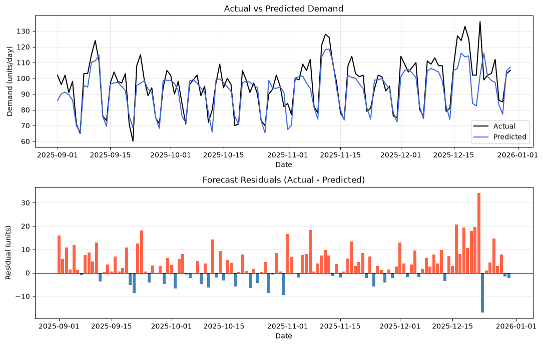

	residual
count	121.00
mean	3.90
std	7.34
min	-16.97
10%	-4.25
50%	3.03
90%	13.00
max	34.19

Reading the results

Measurements and forecasts generally follow the usual period, but residuals become larger before and after events. Even if the average residual is near zero, if the front side hem is long, there is still a risk of shortages. Safety stock reflects the distribution of errors during lead time, not average errors.

No.069: Analyzing the Period When Predictions Fall Short

Meaning in Practice

The cause of a major bad day is either promotion, closure, supply constraints, or master errors, and the approach differs. By linking the upper errors to business events, they can be assigned to feature addition, rule correction, data correction, and approval by the person in charge.

Approach to Analysis and Modeling

The top 10% of absolute error is designated as the “review required date,” and MAE and the number of cases are aggregated by period segment. Thresholds are not for statistical convenience, but are ultimately determined based on operational criteria such as allowable shortages and express costs.

Check with Python

review_threshold = test["abs_error"].quantile(0.90)
test["review_flag"] = test["abs_error"] >= review_threshold
worst_days = test.nlargest(10, "abs_error")[[
    "date", "demand_units", "prediction", "residual", "abs_error",
    "promotion", "special_period"
]]
worst_days_display = worst_days.copy()
worst_days_display[["prediction", "residual", "abs_error"]] = (
    worst_days_display[["prediction", "residual", "abs_error"]].round(1)
)
display(worst_days_display)

period_error = (test.groupby("special_period")
                .agg(days=("date", "size"), MAE=("abs_error", "mean"),
                     review_days=("review_flag", "sum"))
                .sort_values("MAE", ascending=False))
display(period_error.round(2))
print(f"Review threshold (90th percentile): {review_threshold:.2f} units")

	date	demand_units	prediction	residual	abs_error	promotion	special_period
721	2025-12-22	136	101.8	34.2	34.2	0	year_end_rush
715	2025-12-16	127	106.3	20.7	20.7	0	year_end_rush
720	2025-12-21	102	82.4	19.6	19.6	0	year_end_rush
717	2025-12-18	133	113.6	19.4	19.4	0	year_end_rush
676	2025-11-07	112	93.6	18.4	18.4	0	normal
631	2025-09-23	115	97.0	18.0	18.0	0	normal
719	2025-12-20	102	84.1	17.9	17.9	0	year_end_rush
722	2025-12-23	99	116.0	-17.0	17.0	0	normal
670	2025-11-01	84	67.4	16.6	16.6	0	normal
609	2025-09-01	102	86.0	16.0	16.0	0	normal

	days	MAE	review_days
special_period
year_end_rush	7	18.63	5
normal	114	5.40	8

Review threshold (90th percentile): 13.50 units

Reading the results

By looking at the event column for the review date, you can distinguish between recurring factors to be absorbed for model improvement and contingency factors that people should judge as exceptions. Since shipment performance under supply constraints does not represent latent demand, integration with out-of-stock and backlog data is necessary before model adjustments. The top margin of error table can also be used for retrospective meetings in sales, production, and purchasing.

No.070: Linking Demand Forecasting to Inventory and Order Planning

Meaning in Practice

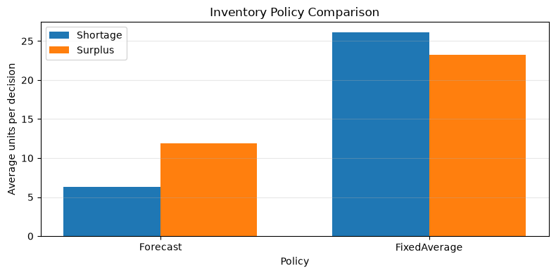
The value of predictive models arises when inventory and emergency response costs are reduced while reducing stockouts. In the final exercise, the forecast value is converted into a place order, simulating the difference from a simple fixed order.

Approach to Analysis and Modeling

Set the lead time to $L=7$ days, and set the order point

$$ROP_t=\sum_{i=1}^{L}\hat{y}_{t+i}+SS, \qquad SS=z\sigma_e\sqrt{L}$$

This approximates the situation. $SS$ is safety stock, $z=1.65$ is the normal approximation with 95% one-sidedness, and $\sigma_e$ is the daily residual standard deviation. To make it easier to understand, we use each test day as the order decision date to evaluate the “quantity needed over the next 7 days,” and compare the forecast base with the average over the past 28 days.

Check with Python

lead_time = 7
z = 1.65
residual_std = test["residual"].std(ddof=1)
safety_stock = z * residual_std * np.sqrt(lead_time)

plan = test[["date", "demand_units", "prediction"]].copy()
plan["actual_lead_demand"] = plan["demand_units"].rolling(lead_time).sum().shift(-(lead_time - 1))
plan["forecast_lead_demand"] = plan["prediction"].rolling(lead_time).sum().shift(-(lead_time - 1))
history_mean = df.set_index("date")["demand_units"].shift(1).rolling(28).mean()
plan["fixed_lead_demand"] = plan["date"].map(history_mean) * lead_time
plan = plan.dropna().copy()

for policy, expected in [("Forecast", "forecast_lead_demand"), ("FixedAverage", "fixed_lead_demand")]:
    plan[f"stock_{policy}"] = plan[expected] + safety_stock
    plan[f"shortage_{policy}"] = (plan["actual_lead_demand"] - plan[f"stock_{policy}"]).clip(lower=0)
    plan[f"surplus_{policy}"] = (plan[f"stock_{policy}"] - plan["actual_lead_demand"]).clip(lower=0)

policy_results = pd.DataFrame({
    "policy": ["Forecast", "FixedAverage"],
    "service_level_pct": [
        100 * (plan["shortage_Forecast"] == 0).mean(),
        100 * (plan["shortage_FixedAverage"] == 0).mean(),
    ],
    "avg_shortage_units": [plan["shortage_Forecast"].mean(), plan["shortage_FixedAverage"].mean()],
    "avg_surplus_units": [plan["surplus_Forecast"].mean(), plan["surplus_FixedAverage"].mean()],
})
print(f"Safety stock: {safety_stock:.1f} units (z={z}, lead time={lead_time} days)")
display(policy_results.set_index("policy").round(2))

fig, ax = plt.subplots(figsize=(8, 4))
x = np.arange(len(policy_results))
ax.bar(x - 0.18, policy_results["avg_shortage_units"], 0.36, label="Shortage")
ax.bar(x + 0.18, policy_results["avg_surplus_units"], 0.36, label="Surplus")
ax.set_title("Inventory Policy Comparison")
ax.set_xlabel("Policy")
ax.set_ylabel("Average units per decision")
ax.set_xticks(x, policy_results["policy"])
ax.grid(True, axis="y", alpha=0.3)
ax.legend()
plt.tight_layout()
plt.show()

Safety stock: 32.1 units (z=1.65, lead time=7 days)

	service_level_pct	avg_shortage_units	avg_surplus_units
policy
Forecast	73.04	6.35	11.85
FixedAverage	63.48	26.13	23.27

Reading the results

By comparing service levels, average shortages, and average surplus simultaneously, accuracy metrics can be translated into inventory determination. Increasing safety stock reduces shortages but increases surplus, so you should set costs for one out-of-stock item and one inventory unit when choosing. This simplified calculation is an independent daily comparison and extends in actual operations to inventory trend simulations including inventory balance, expected arrivals, minimum lots, order intervals, and best-before and storage periods.

Practical Implications Seen Through Target Exercise

1. Aligning granularity with decision-making: Daily, weekly, and monthly are not superior or inferior; their uses differ.
2. Setting a Reference Model: Advanced models that do not exceed the performance of one week ago do not justify the operating costs.
3. follow chronological order: Moving averages that include random partitions or future information tend to overestimate the accuracy of the actual data.
4. Don’t just look at average accuracy: The period of missed and the direction of error determine the risk of out-of-stock items.
5. KPItranslate to business operations: Connect from MAE to service levels, surplus, and express costs to make investment decisions.

What is necessary for practical implementation

• Standardize the definitions and granularity of orders, shipments, stockouts, lost orders, inventory, promotions, and business calendars
• Set a forecast reference date and save only the data available at that time
• Design forecast periods, update frequency, and evaluation metrics based on SKU characteristics and lead times
• Monitor for accuracy degradation, missing measurements, and abnormal values, and record the reasons for personnel overwriting
• Verify ordering rules including out-of-stock costs, storage costs, disposal costs, minimum lot sizes, and capacity constraints.
• Rather than competing solely on accuracy in PoC, design to differentiate from existing operations, define responsibilities, and support retention.

Conclusion

From No.061 to No.070, we checked everything in a single flow: from daily performance observation to aggregation, trend and seasonality, lag features, regression forecasting, time series verification, error cause analysis, and inventory policy comparison. Demand forecasting is not a standalone model but a decision-making system composed of data definition, on-site knowledge, evaluation design, and ordering rules. First, visualizing baseline values and exceptions for small target SKUs and measuring effectiveness through business KPIs is the shortcut to implementation.

Consultations for Corporations

At Suri Kobo, we support everything from problem organization to PoC and operational design in manufacturing related to demand forecasting, inventory optimization, production planning, data infrastructure development, and in-house training. You can consult with us from the stage where you may feel like “We have data but it doesn’t lead to ordering decisions” or “We want to design evaluation indicators that can be used on site.”

📩 Contact Us: surikobo.co.jp/contact
Please feel free to consult us first.