Customer segment analysis and product recommendations to enhance manufacturing proposals

Machine Learning 100-Word Exercise No.081–No.090: Clustering, Similar Search, Collaborative Filtering

This practical section uses customer attributes, transaction records, and product specifications held by equipment and parts manufacturers to transform “Which customer, which product, and why” into reproducible analyses. Connect KMeans, PCA, similarity, user× item matrices, and collaborative filtering into a single sales planning scenario.

The data and analysis results handled in this notebook are fictional examples for training purposes. Recommendation results are candidates that support sales decisions and are not automatically accepted conclusions.

[!NOTE] This material is a notebook previously used by Surikoubo (or personally by the representative, Kazuyama), and has been reconstructed, edited, and published with the company’s permission.
All data listed is fictional and has no relation whatsoever to real companies, factories, or figures.

1. Introduction: Practical Challenges in Manufacturing Covered in This Article

In corporate sales in manufacturing, the more customers and products you have, the harder it becomes to seize proposal opportunities based solely on the experience of the person in charge. In this article, we imagine a situation where the sales planning department of an industrial equipment manufacturer understands the client company, searches for similar customers and products, and develops the next proposal candidate based on the purchase history.

The goal is not to “create a recommendation model.” It is about creating decision-making materials to allocate limited sales man-hours to candidates with a high degree of alignment with customer issues.

2. Common Situations on Site

• Customer segments are limited to sales scale and do not reflect differences in equipment configuration or maintenance issues.
• Product searches rely on model numbers and the memory of the person in charge, overlooking substitutes and related items.
• Purchase history is in the core system but cannot be utilized to suggest unpurchased items.
• They can issue the number of recommendations, but do not quantitatively evaluate whether they were correct.

3. Why is this issue difficult to judge?

“Similar” includes multiple definitions such as sales scale, number of units, downtime losses, quality requirements, product specifications, and purchasing patterns. Also, not having a purchase does not mean unnecessary; it may simply be an unproposed, unrenewed, or purchased from another company. Therefore, it is important not to interpret distance or forecast scores out of touch with the business context.

4. The overall picture of exercise covered this time

No.	technique	Connecting to decision-making
081〜085	KMeans, Cluster Count Assessment, PCA	Understanding the customer base and designing sales strategies
086〜087	Cosine Similarity & Neighborhood Search	Searching for similar products and customers
088〜089	Purchase queue and collaborative filtering	Ranking Cross-Sell Candidates
090	Precision@K/Recall@K	Verification of whether to introduce recommendation measures

5. Preparing the Python environment

We do not use external data or seaborn. Fix the random number generator to 42 so you can reproduce the same results. Standardization is necessary so that different features of the unit do not dominate distance.

import sys
import numpy as np
import pandas as pd
import matplotlib
import matplotlib.pyplot as plt

from sklearn.cluster import KMeans
from sklearn.decomposition import PCA
from sklearn.metrics import silhouette_score
from sklearn.metrics.pairwise import cosine_similarity
from sklearn.preprocessing import StandardScaler

SEED = 42
rng = np.random.default_rng(SEED)
plt.rcParams["figure.figsize"] = (8, 4.8)
plt.rcParams["axes.unicode_minus"] = False

print(f"Python      : {sys.version.split()[0]}")
print(f"NumPy       : {np.__version__}")
print(f"pandas      : {pd.__version__}")
print(f"matplotlib  : {matplotlib.__version__}")

Python      : 3.13.1
NumPy       : 2.5.1
pandas      : 3.0.3
matplotlib  : 3.11.0

6. Creation of Fictional Data

For 120 client companies, it generates annual purchase amounts, equipment units, preventive maintenance ratios, quality requirements, and downtime losses. There are three groups of potential: ‘small scale, price focused,’ ‘medium scale, balanced,’ and ‘large-scale, stable operation priority,’ but the correct answer label is not used for analysis.

Additionally, we will create specification data for 12 products and past purchase statuses. Purchase probability varies depending on customer characteristics and product category fit, simulating a sparse real-world purchase queue.

n_customers = 120
segment = np.repeat([0, 1, 2], [40, 45, 35])
params = {
    0: ([25, 12, 0.30, 45, 1.5], [7, 4, .10, 9, .5]),
    1: ([70, 32, 0.58, 68, 4.5], [13, 7, .10, 8, 1.0]),
    2: ([155, 68, 0.82, 87, 10.0], [25, 12, .07, 5, 2.0]),
}
raw = np.vstack([rng.normal(params[s][0], params[s][1]) for s in segment])
raw[:, 0:2] = np.maximum(raw[:, 0:2], 1)
raw[:, 2] = np.clip(raw[:, 2], 0.05, 0.98)
raw[:, 3] = np.clip(raw[:, 3], 20, 100)
raw[:, 4] = np.maximum(raw[:, 4], 0.2)

feature_cols = ["annual_purchase_mjpy", "installed_machines", "preventive_ratio", "quality_requirement", "downtime_loss_mjpy"]
customers = pd.DataFrame(raw, columns=feature_cols)
customers.insert(0, "customer_id", [f"C{i:03d}" for i in range(1, n_customers + 1)])
customers.head().round(2)

	customer_id	annual_purchase_mjpy	installed_machines	preventive_ratio	quality_requirement	downtime_loss_mjpy
0	C001	27.13	7.84	0.38	53.47	0.52
1	C002	15.88	12.51	0.27	44.85	1.07
2	C003	31.16	15.11	0.31	55.15	1.73
3	C004	18.98	13.48	0.20	52.91	1.48
4	C005	23.71	9.28	0.42	43.61	1.29

products = pd.DataFrame({
    "product_id": [f"P{i:02d}" for i in range(1, 13)],
    "product_name": ["Standard Sensor", "High-precision sensors", "Heat resistance sensor", "Standard motor", "Energy-saving motor", "High-torque motor",
                     "Simple Monitoring Terminal", "Predictive Preservation Terminal", "Quality Inspection Camera", "Replacement parts kit", "Remote Maintenance Contract", "Energy-saving diagnosis"],
    "category": ["sensor"]*3 + ["motor"]*3 + ["digital"]*3 + ["service"]*3,
    "price_index": [25, 58, 62, 45, 70, 76, 30, 82, 88, 18, 55, 48],
    "precision": [45, 88, 72, 50, 65, 70, 42, 78, 95, 35, 60, 55],
    "durability": [50, 68, 92, 64, 75, 90, 45, 80, 68, 55, 70, 50],
    "digital_level": [25, 45, 35, 20, 45, 25, 65, 95, 85, 15, 90, 72],
})

affinity = np.column_stack([
    0.8 - customers["quality_requirement"].to_numpy()/150,
    customers["installed_machines"].to_numpy()/100,
    (customers["preventive_ratio"].to_numpy() + customers["quality_requirement"].to_numpy()/100)/2,
    customers["preventive_ratio"].to_numpy(),
])
cat_index = products["category"].map({"sensor":0, "motor":1, "digital":2, "service":3}).to_numpy()
base = affinity[:, cat_index] + (100-products["price_index"].to_numpy())[None, :] / 500
prob = np.clip(0.08 + 0.48*base + rng.normal(0, .04, (n_customers, 12)), .03, .82)
purchase = (rng.random((n_customers, 12)) < prob).astype(int)
purchase_df = pd.DataFrame(purchase, index=customers.customer_id, columns=products.product_id)

print("number_of_customers:", len(customers), "Number of products:", len(products))
print("Density of purchase queues:", f"{purchase.mean():.1%}")
products

Number of customers: 120 Number of products: 12
Queue density for purchases: 35.4%

	product_id	product_name	category	price_index	precision	durability	digital_level
0	P01	Standard Sensor	sensor	25	45	50	25
1	P02	High-precision sensors	sensor	58	88	68	45
2	P03	Heat resistance sensor	sensor	62	72	92	35
3	P04	Standard motor	motor	45	50	64	20
4	P05	Energy-saving motor	motor	70	65	75	45
5	P06	High-torque motor	motor	76	70	90	25
6	P07	Simple Monitoring Terminal	digital	30	42	45	65
7	P08	Predictive Preservation Terminal	digital	82	78	80	95
8	P09	Quality Inspection Camera	digital	88	95	68	85
9	P10	Replacement parts kit	service	18	35	55	15
10	P11	Remote Maintenance Contract	service	55	60	70	90
11	P12	Energy-saving diagnosis	service	48	55	50	72

No.081: Clustering Customers with KMeans

Meaning in Practice

By organizing customer groups with data, you can design assignments, seminar content, and proposal templates for each group. We create meaningful axes for sales measures, including not only sales but also maintenance maturity and downtime losses.

Approach to Analysis and Modeling

KMeans assigns each customer to the nearest center of gravity, minimizing the sum of squares within the cluster. After standardizing the features, they are divided into three groups and interpreted back to the mean values of the original units.

Check with Python

scaler = StandardScaler()
X = scaler.fit_transform(customers[feature_cols])
kmeans = KMeans(n_clusters=3, random_state=SEED, n_init=20)
customers["cluster"] = kmeans.fit_predict(X)
cluster_profile = customers.groupby("cluster")[feature_cols].agg(["mean", "count"])
cluster_profile.round(2)

	annual_purchase_mjpy		installed_machines		preventive_ratio		quality_requirement		downtime_loss_mjpy
	mean	count	mean	count	mean	count	mean	count	mean	count
cluster
0	69.28	45	31.49	45	0.60	45	67.09	45	4.50	45
1	148.36	35	69.05	35	0.83	35	86.00	35	10.15	35
2	25.22	40	11.85	40	0.28	40	46.73	40	1.42	40

Reading the results

By looking at cluster averages, you can verbalize not only scale but also combinations of conservation and quality requirements. There is no order in the numbers themselves. In sales planning, each group is given names that lead to action, such as ‘Efficient Operation Type,’ ‘Growth Equipment Type,’ and ‘Stable Operation Emphasis Type,’ with stakeholders.

No.082: Determining the Number of Clusters Using the Elbow Method

Meaning in Practice

If you first set the number of clusters as 3, it tends to be classified according to organizational needs. As complexity increases, we check how much variation within the group improves.

Approach to Analysis and Modeling

The objective function is $\mathrm{SSE}=\sum_k\sum_{i\in C_k}\lVert x_i-\mu_k\rVert^2$. Since SSE will inevitably decrease as the number of clusters increases, a bend where the decline is gradual is considered a candidate.

Check with Python

ks = range(1, 9)
inertias = [KMeans(n_clusters=k, random_state=SEED, n_init=20).fit(X).inertia_ for k in ks]
plt.plot(list(ks), inertias, marker="o")
plt.title("Elbow method for customer clusters")
plt.xlabel("Number of clusters k")
plt.ylabel("Within-cluster SSE")
plt.grid(True, alpha=.3)
plt.tight_layout()
plt.show()
pd.DataFrame({"k": list(ks), "SSE": np.round(inertias, 1)})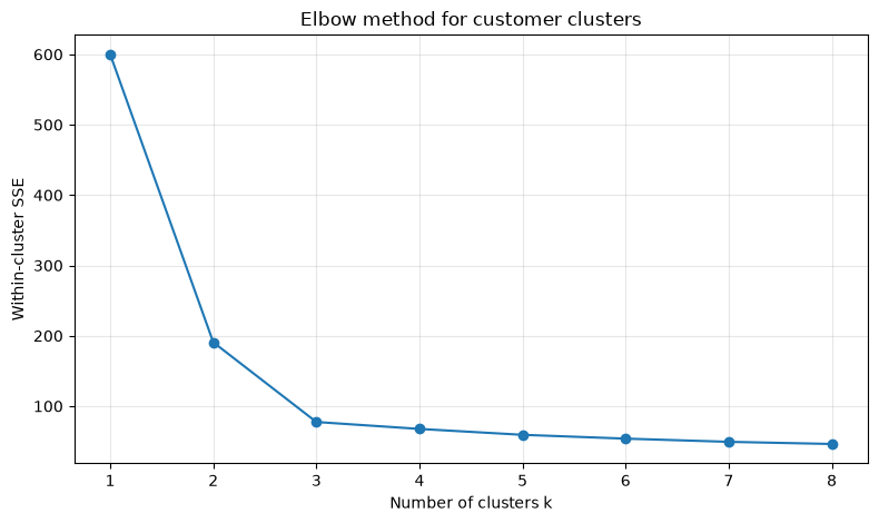

	k	SSE
0	1	600.0
1	2	190.7
2	3	77.4
3	4	67.6
4	5	59.2
5	6	53.8
6	7	49.2
7	8	46.2

Reading the results

Compare the sections with the largest improvement in SSE with those that followed with a gradual progression. Bending is not the only correct answer. You also determine the number of initiatives the sales organization can implement and the minimum number of customers for each group.

No.083: Check the silhouette coefficient

Meaning in Practice

Not only does the elbow method visually inspect, but it also quantifies whether each customer is grouped within their group and apart from others. It can also be used to make decisions to treat boundary customers as exceptions.

Approach to Analysis and Modeling

For each point, if we $a(i)$ the average distance to the same cluster and $b(i)$ the average distance to the nearest cluster, we get $s(i)=(b(i)-a(i))/\max(a(i),b(i))$. The closer to 1, the clearer the separation.

Check with Python

silhouette_rows = []
for k in range(2, 9):
    labels = KMeans(n_clusters=k, random_state=SEED, n_init=20).fit_predict(X)
    silhouette_rows.append((k, silhouette_score(X, labels)))
silhouette_df = pd.DataFrame(silhouette_rows, columns=["k", "silhouette"])
print(silhouette_df.round(3).to_string(index=False))
best_k = int(silhouette_df.loc[silhouette_df.silhouette.idxmax(), "k"])
print(f"\nCandidates for the highest value: k={best_k}")

 k  silhouette
 2       0.597
 3       0.600
 4       0.507
 5       0.385
 6       0.276
 7       0.255
 8       0.256

Maximum candidate: k=3

Reading the results

K, with the highest coefficient, is a statistically strong candidate. However, if the margin is close, simplicity of operation can be prioritized. A low coefficient does not necessarily mean failure; it indicates that customers are continuously changing and may lack a clear group.

No.084: Reducing Dimensions with PCA

Meaning in Practice

Five customer metrics are compressed into two axes, making it easier to explain customer differences. Not only for the clarity of the dashboard, but also to check which variables form the axes.

Approach to Analysis and Modeling

PCA projects data in the orthogonal direction where the variance is maximized. We confirm the contribution rates and loadings of the first and second principal components, and clearly indicate the amount of information lost in two dimensions. Even if the principal component signs are reversed, the meaning remains the same.

Check with Python

pca = PCA(n_components=2)
X_pca = pca.fit_transform(X)
loadings = pd.DataFrame(pca.components_.T, index=feature_cols, columns=["PC1", "PC2"])
print("contribution rate:", np.round(pca.explained_variance_ratio_, 3))
print("Cumulative contribution rate:", round(pca.explained_variance_ratio_.sum(), 3))
loadings.round(3)

Contribution Rate: [0.885 0.04]
Cumulative contribution rate: 0.926

	PC1	PC2
annual_purchase_mjpy	0.450	-0.347
installed_machines	0.456	-0.346
preventive_ratio	0.441	0.492
quality_requirement	0.440	0.610
downtime_loss_mjpy	0.449	-0.382

Reading the results

We look at the cumulative contribution rate to determine how much the two-axis display retains the original information. For features with large absolute load values, PC1 and PC2 are translated into business terms such as ‘scale/importance’ and ‘maintenance attitude.‘

No.085: Visualizing Clusters in Two Dimensions

Meaning in Practice

By visualizing cluster overlap or disconnected customers, you can direct boundary customers who are difficult to apply standard measures to sales reviews.

Approach to Analysis and Modeling

PCA coordinates are used as scatter plots, and KMeans quotas are represented by color. PCA is used for visualization, and clustering is done in standardized 5D, so it’s important that it is not retrained using only 2D.

Check with Python

fig, ax = plt.subplots()
for c in sorted(customers.cluster.unique()):
    mask = customers.cluster.to_numpy() == c
    ax.scatter(X_pca[mask, 0], X_pca[mask, 1], label=f"Cluster {c}", alpha=.75)
ax.set_title("Customer clusters projected onto PCA space")
ax.set_xlabel("Principal component 1")
ax.set_ylabel("Principal component 2")
ax.grid(True, alpha=.3)
ax.legend()
plt.tight_layout()
plt.show()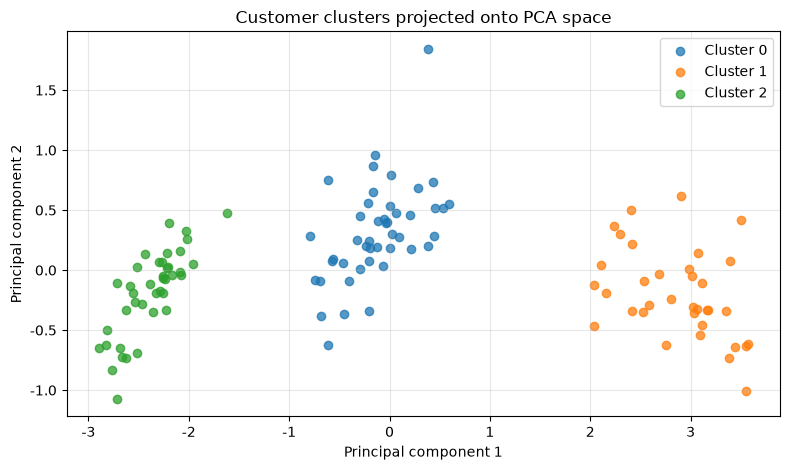

Reading the results

If the flock is generally divided, it becomes easier to explain the strategy. Overlapping points should not be immediately labeled as ‘misclassifications’ but are candidates for multiple initiatives. The distance shown in the figure is after projection onto two components, so it does not match the original 5D distance.

No.086: Search for Similar Products

Meaning in Practice

For discontinued replacements, higher-end models, and set proposals, it is necessary to quickly list products with similar specifications. It can assist with personalized model number knowledge.

Approach to Analysis and Modeling

Standardize price, accuracy, durability, and digitality, and search for products with similar vector orientations by cosine similarity. Categories are intentionally excluded to allow the discovery of candidates beyond categories.

Check with Python

product_features = ["price_index", "precision", "durability", "digital_level"]
Xp = StandardScaler().fit_transform(products[product_features])
product_sim = cosine_similarity(Xp)
query_idx = products.index[products.product_name == "Predictive Preservation Terminal"][0]
order = np.argsort(product_sim[query_idx])[::-1]
similar_products = products.loc[order[order != query_idx][:4], ["product_id", "product_name", "category"]].copy()
similar_products["cosine_similarity"] = product_sim[query_idx, order[order != query_idx][:4]]
similar_products.round(3)

	product_id	product_name	category	cosine_similarity
8	P09	Quality Inspection Camera	digital	0.866
10	P11	Remote Maintenance Contract	service	0.670
4	P05	Energy-saving motor	motor	0.500
1	P02	High-precision sensors	sensor	0.314

Reading the results

The top candidates are not ‘equivalents,’ but those close in terms of specification space. Compatibility, safety standards, and equipment connection conditions are further narrowed down by separate rules. Similar searches broaden the scope of sales exploration, and the final decision is made by technical staff for safer design.

No.087: Search for Similar Customers

Meaning in Practice

When new clients or changes in responsibilities, if you can refer to case studies from similar existing customers, you can quickly create hypotheses for your initial proposal.

Approach to Analysis and Modeling

Use standardized Euclidean distances for customer features. Since we seek customers with similar management and facility characteristics rather than purchase history itself, the recommendation is based on a basis different from later collaborative filtering.

Check with Python

query_customer = "C050"
q = customers.index[customers.customer_id == query_customer][0]
dist = np.linalg.norm(X - X[q], axis=1)
nearest = np.argsort(dist)[1:6]
similar_customers = customers.loc[nearest, ["customer_id", "cluster"] + feature_cols].copy()
similar_customers.insert(2, "distance", dist[nearest])
print("Source of search")
display(customers.loc[[q], ["customer_id", "cluster"] + feature_cols].round(2))
print("Close Customers")
similar_customers.round(2)

Source of search

	customer_id	cluster	annual_purchase_mjpy	installed_machines	preventive_ratio	quality_requirement	downtime_loss_mjpy
49	C050	0	53.26	24.32	0.76	91.24	3.33

Close Customers

	customer_id	cluster	distance	annual_purchase_mjpy	installed_machines	preventive_ratio	quality_requirement	downtime_loss_mjpy
46	C047	0	1.04	50.98	27.87	0.61	77.65	3.77
67	C068	0	1.15	54.18	27.30	0.61	77.24	5.11
54	C055	0	1.25	60.62	34.22	0.57	84.75	6.07
56	C057	0	1.29	76.24	19.79	0.67	71.64	3.39
61	C062	0	1.37	56.31	29.66	0.71	72.66	6.23

Reading the results

Success stories from close customers serve as hypothetical proposals, but contract terms and industry regulations are not necessarily the same. In search results, also include ‘features that provided the basis for similarity,’ so that sales can explain the situation.

No.088: Creating a user × item queue

Meaning in Practice

Convert the purchase history used as input for recommendations into a matrix with customers by row and product columns. This is a critical practical step for determining the granularity, duplication, and return processing of core data.

Approach to Analysis and Modeling

This time, we’ll use implicit feedback where buying is 1 and no is 0. 0 is not a low rating, but unobserved. When using purchase quantities or amounts, conversion is necessary so that only large customers do not control distance.

Check with Python

matrix_preview = purchase_df.iloc[:10].copy()
matrix_preview["purchased_items"] = matrix_preview.sum(axis=1)
matrix_preview

product_id	P01	P02	P03	P04	P05	P06	P07	P08	P09	P10	P11	P12	purchased_items
customer_id
C001	1	0	0	0	0	0	0	1	0	1	1	0	4
C002	1	1	0	1	0	0	0	0	0	0	0	1	4
C003	0	0	1	0	1	0	1	1	1	0	0	1	6
C004	1	1	0	0	0	0	1	1	1	0	0	0	5
C005	0	0	1	0	0	0	0	0	0	0	1	0	2
C006	1	0	0	1	0	1	0	0	0	0	1	1	5
C007	0	1	0	0	0	0	0	0	0	0	0	0	1
C008	0	1	0	1	0	0	0	0	1	0	0	0	3
C009	0	1	0	1	0	0	1	0	1	0	0	1	5
C010	0	0	1	0	0	0	1	0	0	1	0	0	3

Reading the results

Most matrices are sparse matrices that are zero. Monitor density, zero-purchase customers, and zero-purchase products. Integrating browsing and estimate histories increases information, but it is necessary to define the weight of each action and the purposes of personal information and contractual use.

No.089: Implementing Collaborative Filtering

Meaning in Practice

By nominating products purchased by customers with similar purchasing patterns, you can discover cross-selling opportunities that cannot be seen through attribute data alone.

Approach to Analysis and Modeling

$w_{uv}$ cosine similarity between customers, $r_{vi}$ product $i$ purchases $v$ customers, and score by $\hat r_{ui}=\sum_v w_{uv}r_{vi}/\sum_v|w_{uv}|$. Items already purchased will be excluded from the list of candidates.

Check with Python

def recommend_user_based(matrix, customer_id, k=5, neighbor_n=15):
    sim = cosine_similarity(matrix)
    u = matrix.index.get_loc(customer_id)
    neighbors = np.argsort(sim[u])[::-1]
    neighbors = neighbors[(neighbors != u)][:neighbor_n]
    weights = sim[u, neighbors]
    scores = weights @ matrix.iloc[neighbors].to_numpy() / (np.abs(weights).sum() + 1e-12)
    scores[matrix.iloc[u].to_numpy() > 0] = -np.inf
    top = np.argsort(scores)[::-1][:k]
    result = products.set_index("product_id").loc[matrix.columns[top], ["product_name", "category"]].copy()
    result["recommendation_score"] = scores[top]
    return result

recommend_user_based(purchase_df, "C050", k=5).round(3)

	product_name	category	recommendation_score
product_id
P08	Predictive Preservation Terminal	digital	0.511
P05	Energy-saving motor	motor	0.439
P12	Energy-saving diagnosis	service	0.421
P10	Replacement parts kit	service	0.377
P07	Simple Monitoring Terminal	digital	0.337

Reading the results

The score is not the purchase probability itself, but a ranking indicator. As reasons for recommendation, present the number of nearby customers and similar cases. Since new customers and new products have no history of cold starts, they are used together with attribute-based candidates No.086 and 087.

No.090: Evaluating Recommendation Results in Precision@K and Recall@K

Meaning in Practice

Before introducing recommendations, hide some past purchases and measure whether they can be rediscovered through top K purchases. If your sales contact is limited, focus on Precision; if you want to avoid missed opportunities, prioritize Recall.

Approach to Analysis and Modeling

If the top K set of customer $u$ is $R_u@K$ and the test period purchase set is $T_u$, then $\mathrm{Precision@K}=|R_u@K\cap T_u|/K$ and $\mathrm{Recall@K}=|R_u@K\cap T_u|/|T_u|$ are the values.

Check with Python

def offline_evaluate(matrix, k=3, seed=42):
    local_rng = np.random.default_rng(seed)
    train = matrix.copy()
    heldout = {}
    for cid in matrix.index:
        bought = np.flatnonzero(matrix.loc[cid].to_numpy())
        if len(bought) >= 2:
            test_i = int(local_rng.choice(bought))
            train.iloc[train.index.get_loc(cid), test_i] = 0
            heldout[cid] = matrix.columns[test_i]
    sim = cosine_similarity(train)
    precisions, recalls = [], []
    for cid, true_item in heldout.items():
        u = train.index.get_loc(cid)
        neighbors = np.argsort(sim[u])[::-1]
        neighbors = neighbors[(neighbors != u)][:15]
        w = sim[u, neighbors]
        scores = w @ train.iloc[neighbors].to_numpy() / (np.abs(w).sum() + 1e-12)
        scores[train.iloc[u].to_numpy() > 0] = -np.inf
        recs = set(train.columns[np.argsort(scores)[::-1][:k]])
        hit = int(true_item in recs)
        precisions.append(hit / k)
        recalls.append(hit)  # held-out item is one item
    return len(heldout), np.mean(precisions), np.mean(recalls)

rows = []
for k in [1, 3, 5]:
    n, precision, recall = offline_evaluate(purchase_df, k=k)
    rows.append((k, n, precision, recall))
evaluation = pd.DataFrame(rows, columns=["K", "evaluated_customers", "Precision@K", "Recall@K"])
evaluation.round(3)

	K	evaluated_customers	Precision@K	Recall@K
0	1	118	0.169	0.169
1	3	118	0.144	0.432
2	5	118	0.132	0.661

Reading the results

Generally, increasing the K makes Recall easier to rise and Precision more likely to fall. This simple random hold is a learning demo. In practice, we split the process at the point in time, use popularity recommendations and current sales rules as baselines, and ultimately conduct A/B tests on negotiation rates, gross profit, and churn control.

7. Practical Insights Seen Through Target Exercise

1. Segments and recommendations have different roles: Clusters are units for policy design, while recommendations are candidate rankings for each client. Connecting both allows for both overall initiatives and individual proposals.
2. Do not pinpoint similarities into one: Equipment and business characteristics, product specifications, and purchasing patterns are evidence of differences. Integrating multiple candidates and displaying evidence is more trusted in practice.
3. Not considering unpurchased items as refusals: Zero purchases include unproposed, purchased from other companies, or before the renewal period. You need to include the business negotiation history and equipment compatibility conditions.
4. Connecting evaluation metrics with sales capability: K is determined not by model circumstances, but by the number of candidates that one person can confirm or contact.

8. What is necessary for practical implementation

• Data definition: Managing customer and product name tags, handling returns and free items, purchase timing, and discontinued or compatibility information
• Secure candidate generation: Rules first exclude equipment compatibility, safety standards, supply availability, and contract constraints
• Verification that adheres to the time axis: Prevent the mixing of future information, learn from the past, and evaluate future purchases
• On-site operation: Implement candidate fields, rationale, exclusion reasons, and feedback input fields in the CRM
• KPIDesign: Monitor not only Precision@K but also hiring rates, negotiation rates, gross margin, customer satisfaction, and recommendation bias.
• Governance: Define the purpose of use, access rights, retention period, responsibility for model updates, and suspension criteria

For small-scale deployments, starting with a single sales team and product group, starting with monthly candidate lists and manual reviews makes it easier to assess effectiveness and risks.

9. Summary

For No.081–090, we understood the customer structure through clustering, explained it using PCA, created proposal candidates through similarity search and collaborative filtering, and evaluated them using Precision@K and Recall@K. What matters more than advanced algorithms is the definition of similarity, operational constraints, punctual evaluations, and reasons explainable by salespeople.

10. Consultations for Corporations

At Suri Kobo, you can consult on everything from customer segment design in manufacturing, searching for similar products, cross-selling recommendations, PoC evaluation design, to business implementation. We can handle inventory of existing data or small-scale reviews based on existing sales rules as a baseline.

📩 Contact Us: surikobo.co.jp/contact
Please feel free to consult us first.