
100本ノック / 異常検知 / 異常検知100本ノック
製造業の異常検知をPythonで実践|機械学習8手法としきい値設計
射出成形設備の予兆を捉える:機械学習による多変量異常検知10本ノック(No.051〜No.060)
概要
温度・振動・電流・油圧を個別の上限値だけで監視すると、「どの値も上限内だが、組み合わせとして不自然」という設備劣化を見逃します。本記事では、架空の射出成形ラインを題材に、6系統の教師なし学習、モデル比較、異常スコアのしきい値設計までを一つの意思決定プロセスとして確認します。
到達点は、最も高精度なモデルを選ぶことだけではありません。点検できる件数、見逃しによる損失、説明可能性、再学習の運用負荷を踏まえ、現場で継続できる監視ルールを作ることです。
[!NOTE] 本資料は、数理工房 (もしくは代表である和山個人) が過去に企業研修において使用した notebook を企業様の許可を得て再構成・編集のうえ公開しています。
掲載データはすべて架空のものであり、実在する企業・工場・数値とは一切関係ありません。
はじめに:この記事で扱う製造業の実務課題
射出成形設備A-01では、製品1ショットごとにセンサー値を収集しています。保全担当者の目的は、故障を断定することではなく、通常時と異なるショットを早めに絞り込み、計画停止中の点検対象を決めることです。
異常検知モデルの出力は、設備停止命令ではなく点検の優先順位を作る一次スクリーニングとして扱います。センサー校正不良、品種切替、立上げ条件などでもスコアは高くなるため、作業履歴や品質結果との照合が欠かせません。
現場でよくある状況
- 正常データは大量にあるが、故障ラベルは少なく定義も揺れる
- 単一センサーの管理限界では、複数変数の関係崩れを拾えない
- 点検人員には上限があり、アラートを増やしすぎると運用が形骸化する
- 品種、設備、季節、保全後などで「通常」の分布が変わる
なぜこの問題は判断が難しいのか
教師なし異常検知は、正解ラベルを直接学習せず、データの疎らさ・境界・分布から異常度を決めます。したがって同じデータでも、手法とハイパーパラメータによって候補は変わります。また、統計的に珍しいことと、停止や不良につながる業務上の異常は同義ではありません。
今回扱うノックの全体像
| No. | 手法・論点 | 現場で確認すること |
|---|---|---|
| 051 | Isolation Forest | 多変量空間で孤立しやすいショット |
| 052 | Local Outlier Factor | 周辺ショットより局所的に疎な点 |
| 053 | One-Class SVM | 正常領域の柔軟な境界 |
| 054 | Elliptic Envelope | 共分散を考慮した楕円状の正常領域 |
| 055 | k近傍距離 | 近傍までの距離による透明な異常度 |
| 056 | クラスタリング | 小さな群・中心から遠い点の扱い |
| 057 | KMeans | 最寄り中心までの距離で候補抽出 |
| 058 | DBSCAN | 密度の低い領域にあるノイズ点 |
| 059 | モデル比較 | 検出性能・件数・合意度の比較 |
| 060 | しきい値調整 | 点検能力と見逃しコストの反映 |
Python 環境の準備
numpy と pandas でデータを扱い、scikit-learn の各モデルを利用します。グラフは matplotlib のみを使用します。再現性のため乱数シードは42に固定します。
import warnings
import numpy as np
import pandas as pd
import matplotlib
import matplotlib.pyplot as plt
import sklearn

from sklearn.cluster import DBSCAN, KMeans
from sklearn.covariance import EllipticEnvelope
from sklearn.ensemble import IsolationForest
from sklearn.metrics import precision_score, recall_score, f1_score
from sklearn.neighbors import LocalOutlierFactor, NearestNeighbors
from sklearn.pipeline import make_pipeline
from sklearn.preprocessing import StandardScaler
from sklearn.svm import OneClassSVM

warnings.filterwarnings("ignore", category=UserWarning, module="matplotlib")
SEED = 42
np.random.seed(SEED)
pd.set_option("display.max_columns", 20)

print(f"numpy       : {np.__version__}")
print(f"pandas      : {pd.__version__}")
print(f"matplotlib  : {matplotlib.__version__}")
print(f"scikit-learn: {sklearn.__version__}")
numpy : 2.5.1
pandas : 3.0.3
matplotlib : 3.11.0
scikit-learn: 1.9.0架空データの作成
通常900ショット、要確認40ショットを生成します。通常時には、金型温度が上がるとヒーター電流もやや増え、振動と油圧にも弱い関係があると仮定します。要確認データには、振動増加、温度と電流の関係崩れ、油圧低下という複数の劣化パターンを混ぜます。
known_issue は、後日の点検・品質確認で判明した評価用ラベルという設定です。モデル学習には使いません。これは完全な故障ラベルではなく、比較のための限定的な監査結果です。
rng = np.random.default_rng(SEED)
n_normal, n_issue = 900, 40

mean = np.array([210.0, 2.4, 31.0, 8.0])
cov = np.array([
    [16.0, 0.7, 5.0, 1.0],
    [0.7, 0.36, 0.4, 0.3],
    [5.0, 0.4, 9.0, 1.2],
    [1.0, 0.3, 1.2, 1.0],
])
normal = rng.multivariate_normal(mean, cov, n_normal)

issue_1 = rng.multivariate_normal([211, 5.4, 33, 9.4], np.diag([9, .20, 4, .35]), 14)
issue_2 = rng.multivariate_normal([222, 2.7, 25, 8.2], np.diag([8, .25, 3, .50]), 13)
issue_3 = rng.multivariate_normal([207, 3.6, 32, 5.4], np.diag([7, .22, 4, .20]), 13)
issue = np.vstack([issue_1, issue_2, issue_3])

columns = ["mold_temp_c", "vibration_mm_s", "heater_current_a", "oil_pressure_mpa"]
df = pd.DataFrame(np.vstack([normal, issue]), columns=columns)
df.insert(0, "shot_id", [f"S{i:04d}" for i in range(1, len(df) + 1)])
df["known_issue"] = np.r_[np.zeros(n_normal, dtype=int), np.ones(n_issue, dtype=int)]
X = df[columns]
X_scaled = StandardScaler().fit_transform(X)

print(f"ショット数: {len(df):,} / 評価上の要確認: {df['known_issue'].sum()}")
display(df.head())
display(df.groupby("known_issue")[columns].agg(["mean", "std"]).round(2))
ショット数: 940 / 評価上の要確認: 40| shot_id | mold_temp_c | vibration_mm_s | heater_current_a | oil_pressure_mpa | known_issue | |
|---|---|---|---|---|---|---|
| 0 | S0001 | 207.579632 | 2.201556 | 32.597790 | 8.998515 | 0 |
| 1 | S0002 | 215.879777 | 2.994548 | 37.801656 | 9.099905 | 0 |
| 2 | S0003 | 209.024388 | 2.377789 | 32.812262 | 9.146080 | 0 |
| 3 | S0004 | 211.071845 | 2.910164 | 28.307671 | 7.929873 | 0 |
| 4 | S0005 | 207.416243 | 2.676244 | 32.282850 | 8.891665 | 0 |
| mold_temp_c | vibration_mm_s | heater_current_a | oil_pressure_mpa | |||||
|---|---|---|---|---|---|---|---|---|
| mean | std | mean | std | mean | std | mean | std | |
| known_issue | ||||||||
| 0 | 210.04 | 3.88 | 2.4 | 0.59 | 31.04 | 2.99 | 7.98 | 1.02 |
| 1 | 213.47 | 6.42 | 3.9 | 1.25 | 30.52 | 4.45 | 7.63 | 1.75 |
fig, axes = plt.subplots(1, 2, figsize=(12, 4.5))
colors = np.where(df["known_issue"].eq(1), "tab:red", "tab:blue")
axes[0].scatter(df["mold_temp_c"], df["heater_current_a"], c=colors, alpha=.55, s=20)
axes[0].set_title("Temperature vs. heater current")
axes[0].set_xlabel("Mold temperature [C]")
axes[0].set_ylabel("Heater current [A]")
axes[0].grid(True, alpha=.3)
axes[1].scatter(df["vibration_mm_s"], df["oil_pressure_mpa"], c=colors, alpha=.55, s=20)
axes[1].set_title("Vibration vs. oil pressure")
axes[1].set_xlabel("Vibration [mm/s]")
axes[1].set_ylabel("Oil pressure [MPa]")
axes[1].grid(True, alpha=.3)
fig.tight_layout()
plt.show()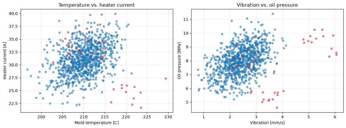
No.051:Isolation Forestを使う
実務での意味
Isolation Forestは、特徴量をランダムに分割したとき少ない分割回数で孤立する点を異常とみなします。正常状態の厳密な分布を仮定しないため、複数センサーが作る複雑な領域から候補を素早く抽出する初期PoCに向きます。
分析・モデル化の考え方
点 の平均経路長を 、標本数 における平均経路長の基準を とすると、代表的な異常度は次式です。
が1に近いほど孤立しやすいと解釈します。contamination=0.05 は「約5%を必ず異常とする」業務仮説であり、故障率の推定値ではありません。
Pythonで確認する
iso = IsolationForest(n_estimators=300, contamination=.05, random_state=SEED)
df["score_iso"] = -iso.fit(X_scaled).score_samples(X_scaled)
df["pred_iso"] = (iso.predict(X_scaled) == -1).astype(int)
display(df.nlargest(8, "score_iso")[["shot_id", *columns, "score_iso", "known_issue"]].round(3))

plt.figure(figsize=(8, 4.5))
plt.scatter(df["mold_temp_c"], df["vibration_mm_s"], c=df["score_iso"], cmap="viridis", s=22)
plt.colorbar(label="Isolation score")
plt.title("Isolation Forest anomaly score")
plt.xlabel("Mold temperature [C]")
plt.ylabel("Vibration [mm/s]")
plt.grid(True, alpha=.3)
plt.tight_layout()
plt.show()| shot_id | mold_temp_c | vibration_mm_s | heater_current_a | oil_pressure_mpa | score_iso | known_issue | |
|---|---|---|---|---|---|---|---|
| 918 | S0919 | 223.604 | 3.687 | 21.653 | 7.238 | 0.696 | 1 |
| 126 | S0127 | 220.592 | 3.633 | 37.847 | 11.397 | 0.672 | 0 |
| 900 | S0901 | 213.905 | 6.052 | 37.836 | 8.578 | 0.651 | 1 |
| 912 | S0913 | 215.102 | 5.515 | 33.103 | 10.246 | 0.630 | 1 |
| 907 | S0908 | 214.681 | 5.932 | 34.262 | 9.830 | 0.629 | 1 |
| 910 | S0911 | 206.332 | 5.110 | 36.330 | 9.347 | 0.621 | 1 |
| 916 | S0917 | 221.522 | 2.150 | 22.260 | 8.207 | 0.620 | 1 |
| 926 | S0927 | 223.477 | 2.998 | 24.598 | 8.074 | 0.620 | 1 |
結果の読み取り
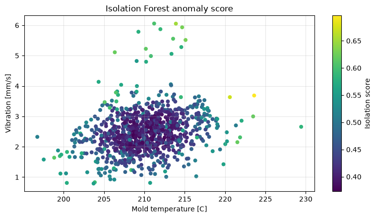
上位には、振動が大きいショットや温度・電流の関係が通常群から離れたショットが含まれます。木の分岐に基づく総合スコアだけでは原因を断定できないため、上位行の元センサー値を併記し、保全担当者が設備履歴と照合できる形にします。
No.052:Local Outlier Factorを使う
実務での意味
LOFは、全体ではなく「近くの運転点と比べて疎か」を評価します。品種や負荷によって複数の正常群がある現場で、ある運転群の中だけで浮いているショットを見つけるのに有効です。
分析・モデル化の考え方
点 の局所到達可能密度を とすると、LOFは近傍との密度比で表せます。
概ね1なら近傍と同程度、1より十分大きいと局所外れ値です。近傍数は工程の連続性やロット規模に合わせて感度分析します。
Pythonで確認する
lof = LocalOutlierFactor(n_neighbors=25, contamination=.05)
df["pred_lof"] = (lof.fit_predict(X_scaled) == -1).astype(int)
df["score_lof"] = -lof.negative_outlier_factor_
display(df.nlargest(8, "score_lof")[["shot_id", *columns, "score_lof", "known_issue"]].round(3))

plt.figure(figsize=(8, 4.5))
plt.scatter(df["vibration_mm_s"], df["oil_pressure_mpa"], c=df["score_lof"], cmap="plasma", s=22)
plt.colorbar(label="LOF score")
plt.title("Local Outlier Factor score")
plt.xlabel("Vibration [mm/s]")
plt.ylabel("Oil pressure [MPa]")
plt.grid(True, alpha=.3)
plt.tight_layout()
plt.show()| shot_id | mold_temp_c | vibration_mm_s | heater_current_a | oil_pressure_mpa | score_lof | known_issue | |
|---|---|---|---|---|---|---|---|
| 922 | S0923 | 229.429 | 2.657 | 27.339 | 8.708 | 2.082 | 1 |
| 918 | S0919 | 223.604 | 3.687 | 21.653 | 7.238 | 2.026 | 1 |
| 126 | S0127 | 220.592 | 3.633 | 37.847 | 11.397 | 2.018 | 0 |
| 901 | S0902 | 211.210 | 6.057 | 34.612 | 8.425 | 1.901 | 1 |
| 900 | S0901 | 213.905 | 6.052 | 37.836 | 8.578 | 1.887 | 1 |
| 478 | S0479 | 204.327 | 4.137 | 36.266 | 9.103 | 1.858 | 0 |
| 903 | S0904 | 209.262 | 5.785 | 32.073 | 8.304 | 1.836 | 1 |
| 907 | S0908 | 214.681 | 5.932 | 34.262 | 9.830 | 1.832 | 1 |
結果の読み取り
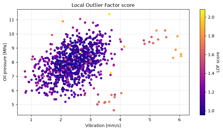
LOF上位は、周辺密度との差が大きい候補です。境界部の正常点も拾いやすいため、n_neighbors を変えたときも順位が安定するか確認します。またLOFは原則として学習データ内の外れ値探索に向くため、新着データ採点では novelty=True を使う別設計が必要です。
No.053:One-Class SVMを使う
実務での意味
One-Class SVMは、多数を占める通常データを囲む境界を学習します。RBFカーネルを使えば非線形な正常領域を表現でき、単純な上下限では捉えにくい関係崩れを検出できます。
分析・モデル化の考え方
特徴空間で原点から正常データを分離する超平面を求めます。概念的な最適化問題は次式です。
は境界外点の割合の上限とサポートベクトル割合の下限に関係します。スケールに敏感なため標準化は必須です。
Pythonで確認する
ocsvm = OneClassSVM(kernel="rbf", gamma="scale", nu=.05)
df["score_ocsvm"] = -ocsvm.fit(X_scaled).decision_function(X_scaled)
df["pred_ocsvm"] = (ocsvm.predict(X_scaled) == -1).astype(int)
display(df.nlargest(8, "score_ocsvm")[["shot_id", *columns, "score_ocsvm", "known_issue"]].round(3))

plt.figure(figsize=(8, 4.5))
plt.hist(df.loc[df.known_issue.eq(0), "score_ocsvm"], bins=35, alpha=.65, label="audit: normal")
plt.hist(df.loc[df.known_issue.eq(1), "score_ocsvm"], bins=20, alpha=.65, label="audit: issue")
plt.axvline(0, color="black", linestyle="--", label="model boundary")
plt.title("One-Class SVM score distribution")
plt.xlabel("Anomaly score (higher = more anomalous)")
plt.ylabel("Shots")
plt.grid(True, alpha=.3)
plt.legend()
plt.tight_layout()
plt.show()| shot_id | mold_temp_c | vibration_mm_s | heater_current_a | oil_pressure_mpa | score_ocsvm | known_issue | |
|---|---|---|---|---|---|---|---|
| 126 | S0127 | 220.592 | 3.633 | 37.847 | 11.397 | 1.347 | 0 |
| 922 | S0923 | 229.429 | 2.657 | 27.339 | 8.708 | 1.345 | 1 |
| 918 | S0919 | 223.604 | 3.687 | 21.653 | 7.238 | 1.174 | 1 |
| 157 | S0158 | 211.063 | 2.070 | 38.227 | 10.885 | 0.730 | 0 |
| 900 | S0901 | 213.905 | 6.052 | 37.836 | 8.578 | 0.668 | 1 |
| 939 | S0940 | 206.474 | 3.786 | 29.456 | 4.601 | 0.452 | 1 |
| 933 | S0934 | 214.528 | 3.633 | 31.250 | 5.200 | 0.419 | 1 |
| 34 | S0035 | 209.778 | 1.705 | 28.220 | 9.928 | 0.408 | 0 |
結果の読み取り
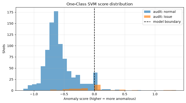
スコア0がモデル境界で、正側ほど要確認です。監査上の正常・要確認の分布には重なりがあり、モデルだけで完全分離できないことも分かります。gamma を大きくしすぎると境界が細かくなり、通常変動にも反応するため注意します。
No.054:Elliptic Envelopeを使う
実務での意味
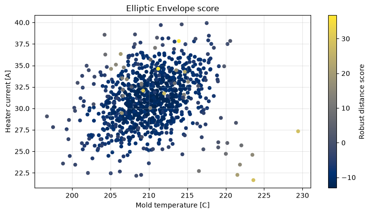
Elliptic Envelopeは、正常データが概ね単峰の楕円状に分布する工程に向きます。共分散を考慮するため、温度と電流がそれぞれ範囲内でも、通常の相関関係から外れた状態を検出できます。
分析・モデル化の考え方
中心 と共分散行列 を用いたマハラノビス距離
をロバストに推定し、距離が大きい点を異常候補にします。多峰性が強い工程では一つの楕円という仮定が崩れます。
Pythonで確認する
ell = EllipticEnvelope(contamination=.05, random_state=SEED)
df["score_elliptic"] = -ell.fit(X_scaled).decision_function(X_scaled)
df["pred_elliptic"] = (ell.predict(X_scaled) == -1).astype(int)
display(df.nlargest(8, "score_elliptic")[["shot_id", *columns, "score_elliptic", "known_issue"]].round(3))

plt.figure(figsize=(8, 4.5))
plt.scatter(df["mold_temp_c"], df["heater_current_a"], c=df["score_elliptic"], cmap="cividis", s=22)
plt.colorbar(label="Robust distance score")
plt.title("Elliptic Envelope score")
plt.xlabel("Mold temperature [C]")
plt.ylabel("Heater current [A]")
plt.grid(True, alpha=.3)
plt.tight_layout()
plt.show()| shot_id | mold_temp_c | vibration_mm_s | heater_current_a | oil_pressure_mpa | score_elliptic | known_issue | |
|---|---|---|---|---|---|---|---|
| 900 | S0901 | 213.905 | 6.052 | 37.836 | 8.578 | 36.750 | 1 |
| 901 | S0902 | 211.210 | 6.057 | 34.612 | 8.425 | 36.431 | 1 |
| 903 | S0904 | 209.262 | 5.785 | 32.073 | 8.304 | 30.518 | 1 |
| 918 | S0919 | 223.604 | 3.687 | 21.653 | 7.238 | 28.626 | 1 |
| 922 | S0923 | 229.429 | 2.657 | 27.339 | 8.708 | 28.577 | 1 |
| 905 | S0906 | 211.985 | 5.871 | 31.745 | 8.877 | 27.169 | 1 |
| 907 | S0908 | 214.681 | 5.932 | 34.262 | 9.830 | 24.147 | 1 |
| 916 | S0917 | 221.522 | 2.150 | 22.260 | 8.207 | 20.851 | 1 |
結果の読み取り
温度と電流の組み合わせが通常の帯から外れた候補が高スコアになります。仮定が明確で説明しやすい一方、品種別に中心が分かれる場合は品種ごとにモデルを分けるか、別の手法を検討します。
No.055:k近傍法で異常度を計算する
実務での意味
k近傍距離は「似た過去ショットがどれだけ近くにあるか」を直接示します。アルゴリズムが比較的透明で、保全担当者に類似ショットを併せて提示しやすい点が利点です。
分析・モデル化の考え方
標準化後の点 と第 近傍 のユークリッド距離を異常度とします。
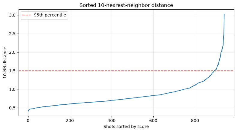
が小さいと局所ノイズに敏感で、大きいと小規模な正常群まで異常扱いしやすくなります。ここでは第10近傍距離を使い、上位5%を候補とします。
Pythonで確認する
knn = NearestNeighbors(n_neighbors=11).fit(X_scaled)
distances, _ = knn.kneighbors(X_scaled)
df["score_knn"] = distances[:, -1]
knn_threshold = df["score_knn"].quantile(.95)
df["pred_knn"] = (df["score_knn"] >= knn_threshold).astype(int)
display(df.nlargest(8, "score_knn")[["shot_id", *columns, "score_knn", "known_issue"]].round(3))

sorted_score = np.sort(df["score_knn"])
plt.figure(figsize=(8, 4.5))
plt.plot(np.arange(1, len(df) + 1), sorted_score)
plt.axhline(knn_threshold, color="tab:red", linestyle="--", label="95th percentile")
plt.title("Sorted 10-nearest-neighbor distance")
plt.xlabel("Shots sorted by score")
plt.ylabel("10-NN distance")
plt.grid(True, alpha=.3)
plt.legend()
plt.tight_layout()
plt.show()| shot_id | mold_temp_c | vibration_mm_s | heater_current_a | oil_pressure_mpa | score_knn | known_issue | |
|---|---|---|---|---|---|---|---|
| 922 | S0923 | 229.429 | 2.657 | 27.339 | 8.708 | 3.021 | 1 |
| 918 | S0919 | 223.604 | 3.687 | 21.653 | 7.238 | 2.670 | 1 |
| 900 | S0901 | 213.905 | 6.052 | 37.836 | 8.578 | 2.457 | 1 |
| 126 | S0127 | 220.592 | 3.633 | 37.847 | 11.397 | 2.433 | 0 |
| 910 | S0911 | 206.332 | 5.110 | 36.330 | 9.347 | 2.355 | 1 |
| 903 | S0904 | 209.262 | 5.785 | 32.073 | 8.304 | 2.189 | 1 |
| 912 | S0913 | 215.102 | 5.515 | 33.103 | 10.246 | 2.164 | 1 |
| 911 | S0912 | 210.178 | 5.224 | 30.045 | 10.242 | 2.156 | 1 |
結果の読み取り
右端で距離が急に増える点は、似た履歴が少ない候補です。分位点しきい値は点検件数を制御しやすい反面、工程がすべて正常でも一定数を抽出します。まず候補リストを作る用途と位置づけます。
No.056:クラスタリングで外れたデータを検出する
実務での意味
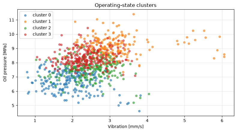
クラスタリングを使うと、主要な運転状態を群として整理し、中心から遠い点や極端に小さい群を調査できます。ただし、小さい群が異常とは限らず、少量品種や段取り直後という正当な運転状態かもしれません。
分析・モデル化の考え方
異常検知への使い方は主に二つです。
- 各点から所属クラスタ中心までの距離を異常度にする
- 所属点数が小さいクラスタを稀な運転状態としてレビューする
クラスタリングは故障判定器ではなく、データ構造を整理する道具です。工程条件を含めた意味付けが必要です。
Pythonで確認する
kmeans_review = KMeans(n_clusters=4, n_init=20, random_state=SEED).fit(X_scaled)
df["cluster_review"] = kmeans_review.labels_
cluster_review = df.groupby("cluster_review").agg(
    shots=("shot_id", "size"),
    issue_rate=("known_issue", "mean"),
    temp_mean=("mold_temp_c", "mean"),
    vibration_mean=("vibration_mm_s", "mean"),
    pressure_mean=("oil_pressure_mpa", "mean"),
).round(3)
display(cluster_review)

plt.figure(figsize=(8, 4.5))
for c in sorted(df["cluster_review"].unique()):
    part = df[df["cluster_review"].eq(c)]
    plt.scatter(part["vibration_mm_s"], part["oil_pressure_mpa"], s=22, alpha=.6, label=f"cluster {c}")
plt.title("Operating-state clusters")
plt.xlabel("Vibration [mm/s]")
plt.ylabel("Oil pressure [MPa]")
plt.grid(True, alpha=.3)
plt.legend()
plt.tight_layout()
plt.show()| shots | issue_rate | temp_mean | vibration_mean | pressure_mean | |
|---|---|---|---|---|---|
| cluster_review | |||||
| 0 | 213 | 0.038 | 207.104 | 1.957 | 6.738 |
| 1 | 211 | 0.066 | 212.647 | 3.125 | 9.144 |
| 2 | 254 | 0.071 | 213.386 | 2.451 | 7.632 |
| 3 | 262 | 0.000 | 207.592 | 2.367 | 8.339 |
結果の読み取り
クラスタ別の件数と監査上の要確認率を見ると、どの運転群を優先レビューすべきか整理できます。ただし要確認率が高い群をそのまま停止条件にはせず、品種・金型・作業条件が偏っていないかを先に調べます。
No.057:KMeansで異常候補を抽出する
実務での意味
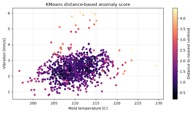
KMeansは、代表的な運転状態の重心を作り、どの重心からも遠いショットを抽出します。複数の定常運転モードがある場合でも、全体平均からの距離より実態に合う可能性があります。
分析・モデル化の考え方
KMeansはクラスタ内平方和
を最小化します。学習後は を異常度とします。クラスタ数 と分位点しきい値は、運転モード数と点検能力を踏まえて決めます。
Pythonで確認する
kmeans = KMeans(n_clusters=4, n_init=20, random_state=SEED).fit(X_scaled)
distance_matrix = kmeans.transform(X_scaled)
df["score_kmeans"] = distance_matrix.min(axis=1)
kmeans_threshold = df["score_kmeans"].quantile(.95)
df["pred_kmeans"] = (df["score_kmeans"] >= kmeans_threshold).astype(int)
display(df.nlargest(8, "score_kmeans")[["shot_id", *columns, "score_kmeans", "known_issue"]].round(3))

plt.figure(figsize=(8, 4.5))
plt.scatter(df["mold_temp_c"], df["vibration_mm_s"], c=df["score_kmeans"], cmap="magma", s=22)
plt.colorbar(label="Distance to nearest centroid")
plt.title("KMeans distance-based anomaly score")
plt.xlabel("Mold temperature [C]")
plt.ylabel("Vibration [mm/s]")
plt.grid(True, alpha=.3)
plt.tight_layout()
plt.show()| shot_id | mold_temp_c | vibration_mm_s | heater_current_a | oil_pressure_mpa | score_kmeans | known_issue | |
|---|---|---|---|---|---|---|---|
| 918 | S0919 | 223.604 | 3.687 | 21.653 | 7.238 | 4.484 | 1 |
| 900 | S0901 | 213.905 | 6.052 | 37.836 | 8.578 | 4.456 | 1 |
| 922 | S0923 | 229.429 | 2.657 | 27.339 | 8.708 | 4.304 | 1 |
| 901 | S0902 | 211.210 | 6.057 | 34.612 | 8.425 | 4.285 | 1 |
| 907 | S0908 | 214.681 | 5.932 | 34.262 | 9.830 | 4.114 | 1 |
| 903 | S0904 | 209.262 | 5.785 | 32.073 | 8.304 | 4.020 | 1 |
| 905 | S0906 | 211.985 | 5.871 | 31.745 | 8.877 | 4.001 | 1 |
| 916 | S0917 | 221.522 | 2.150 | 22.260 | 8.207 | 3.709 | 1 |
結果の読み取り
最近傍重心から遠いショットが上位になります。重心は平均なので外れ値の影響を受けます。本番では、明らかなセンサー故障を前処理で除外し、品種構成が変わった際には重心の再評価が必要です。
No.058:DBSCANでノイズ点を検出する
実務での意味
DBSCANは、十分に密な領域をクラスタとし、どの密集領域にも属さない点をノイズと判定します。クラスタ数を事前に決めず、非球形の運転領域にも対応できる点が特徴です。
分析・モデル化の考え方
半径 内に min_samples 個以上の点がある点をコア点とし、密度到達可能な点を同じクラスタにまとめます。eps が小さすぎるとアラート過多、大きすぎると異常を正常群へ吸収します。標準化後の距離で設定します。
Pythonで確認する
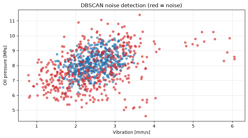
dbscan = DBSCAN(eps=.62, min_samples=12).fit(X_scaled)
df["dbscan_label"] = dbscan.labels_
df["pred_dbscan"] = (df["dbscan_label"] == -1).astype(int)
dbscan_summary = df.groupby("dbscan_label").agg(shots=("shot_id", "size"), issue_rate=("known_issue", "mean")).round(3)
display(dbscan_summary)

plt.figure(figsize=(8, 4.5))
plot_colors = np.where(df["pred_dbscan"].eq(1), "tab:red", "tab:blue")
plt.scatter(df["vibration_mm_s"], df["oil_pressure_mpa"], c=plot_colors, alpha=.6, s=22)
plt.title("DBSCAN noise detection (red = noise)")
plt.xlabel("Vibration [mm/s]")
plt.ylabel("Oil pressure [MPa]")
plt.grid(True, alpha=.3)
plt.tight_layout()
plt.show()| shots | issue_rate | |
|---|---|---|
| dbscan_label | ||
| -1 | 503 | 0.08 |
| 0 | 398 | 0.00 |
| 1 | 26 | 0.00 |
| 2 | 8 | 0.00 |
| 3 | 5 | 0.00 |
結果の読み取り
赤いノイズ点は密な通常領域から外れています。DBSCANは直接の連続スコアを返さず、パラメータ感度も高いため、ノイズ件数が現場の点検能力に収まるか、既知の稀な正常運転を巻き込んでいないかを確認します。
No.059:モデルごとの異常検知結果を比較する
実務での意味
モデル選定では精度だけでなく、アラート件数、見逃し、モデル間の合意、説明のしやすさを比較します。評価ラベルが限定的な場合、数値順位を絶対視せず、複数モデルが共通して挙げる候補を優先監査する方法が実用的です。
分析・モデル化の考え方
監査済みデータに限り、次を確認します。
\mathrm{Recall}=\frac{TP}{TP+FN},\quad F_1=\frac{2PR}{P+R}$$ 異常が少ないためAccuracyは参考にしません。また、同じ件数を出すモデル同士でも候補が一致するとは限りません。 ### Pythonで確認する ```python pred_cols = { "Isolation Forest": "pred_iso", "LOF": "pred_lof", "One-Class SVM": "pred_ocsvm", "Elliptic Envelope": "pred_elliptic", "kNN distance": "pred_knn", "KMeans distance": "pred_kmeans", "DBSCAN": "pred_dbscan", } rows = [] for name, col in pred_cols.items(): rows.append({ "model": name, "alerts": int(df[col].sum()), "precision": precision_score(df["known_issue"], df[col], zero_division=0), "recall": recall_score(df["known_issue"], df[col], zero_division=0), "f1": f1_score(df["known_issue"], df[col], zero_division=0), }) comparison = pd.DataFrame(rows).set_index("model").sort_values("f1", ascending=False) display(comparison.round(3)) comparison[["precision", "recall", "f1"]].plot(kind="bar", figsize=(10, 4.8), ylim=(0, 1)) plt.title("Model comparison on audited labels") plt.xlabel("Model") plt.ylabel("Metric") plt.grid(True, axis="y", alpha=.3) plt.legend(loc="lower right") plt.tight_layout() plt.show() ``` <style scoped> .dataframe tbody tr th:only-of-type { vertical-align: middle; } .dataframe tbody tr th { vertical-align: top; } .dataframe thead th { text-align: right; } </style> <table border="1" class="dataframe"> <thead> <tr style="text-align: right;"> <th></th> <th>alerts</th> <th>precision</th> <th>recall</th> <th>f1</th> </tr> <tr> <th>model</th> <th></th> <th></th> <th></th> <th></th> </tr> </thead> <tbody> <tr> <th>Elliptic Envelope</th> <td>47</td> <td>0.830</td> <td>0.975</td> <td>0.897</td> </tr> <tr> <th>KMeans distance</th> <td>47</td> <td>0.745</td> <td>0.875</td> <td>0.805</td> </tr> <tr> <th>LOF</th> <td>47</td> <td>0.702</td> <td>0.825</td> <td>0.759</td> </tr> <tr> <th>kNN distance</th> <td>47</td> <td>0.660</td> <td>0.775</td> <td>0.713</td> </tr> <tr> <th>Isolation Forest</th> <td>47</td> <td>0.638</td> <td>0.750</td> <td>0.690</td> </tr> <tr> <th>One-Class SVM</th> <td>50</td> <td>0.340</td> <td>0.425</td> <td>0.378</td> </tr> <tr> <th>DBSCAN</th> <td>503</td> <td>0.080</td> <td>1.000</td> <td>0.147</td> </tr> </tbody> </table> 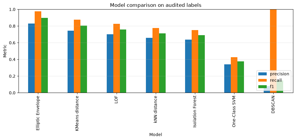 ```python df["model_votes"] = df[list(pred_cols.values())].sum(axis=1) vote_summary = df.groupby("model_votes").agg( shots=("shot_id", "size"), audited_issues=("known_issue", "sum"), issue_rate=("known_issue", "mean"), ).round(3) display(vote_summary) display(df.nlargest(10, "model_votes")[["shot_id", "model_votes", *columns, "known_issue"]].round(3)) ``` <style scoped> .dataframe tbody tr th:only-of-type { vertical-align: middle; } .dataframe tbody tr th { vertical-align: top; } .dataframe thead th { text-align: right; } </style> <table border="1" class="dataframe"> <thead> <tr style="text-align: right;"> <th></th> <th>shots</th> <th>audited_issues</th> <th>issue_rate</th> </tr> <tr> <th>model_votes</th> <th></th> <th></th> <th></th> </tr> </thead> <tbody> <tr> <th>0</th> <td>437</td> <td>0</td> <td>0.000</td> </tr> <tr> <th>1</th> <td>421</td> <td>1</td> <td>0.002</td> </tr> <tr> <th>2</th> <td>20</td> <td>2</td> <td>0.100</td> </tr> <tr> <th>3</th> <td>16</td> <td>4</td> <td>0.250</td> </tr> <tr> <th>4</th> <td>4</td> <td>1</td> <td>0.250</td> </tr> <tr> <th>5</th> <td>7</td> <td>3</td> <td>0.429</td> </tr> <tr> <th>6</th> <td>17</td> <td>14</td> <td>0.824</td> </tr> <tr> <th>7</th> <td>18</td> <td>15</td> <td>0.833</td> </tr> </tbody> </table> <style scoped> .dataframe tbody tr th:only-of-type { vertical-align: middle; } .dataframe tbody tr th { vertical-align: top; } .dataframe thead th { text-align: right; } </style> <table border="1" class="dataframe"> <thead> <tr style="text-align: right;"> <th></th> <th>shot_id</th> <th>model_votes</th> <th>mold_temp_c</th> <th>vibration_mm_s</th> <th>heater_current_a</th> <th>oil_pressure_mpa</th> <th>known_issue</th> </tr> </thead> <tbody> <tr> <th>126</th> <td>S0127</td> <td>7</td> <td>220.592</td> <td>3.633</td> <td>37.847</td> <td>11.397</td> <td>0</td> </tr> <tr> <th>157</th> <td>S0158</td> <td>7</td> <td>211.063</td> <td>2.070</td> <td>38.227</td> <td>10.885</td> <td>0</td> </tr> <tr> <th>478</th> <td>S0479</td> <td>7</td> <td>204.327</td> <td>4.137</td> <td>36.266</td> <td>9.103</td> <td>0</td> </tr> <tr> <th>900</th> <td>S0901</td> <td>7</td> <td>213.905</td> <td>6.052</td> <td>37.836</td> <td>8.578</td> <td>1</td> </tr> <tr> <th>901</th> <td>S0902</td> <td>7</td> <td>211.210</td> <td>6.057</td> <td>34.612</td> <td>8.425</td> <td>1</td> </tr> <tr> <th>903</th> <td>S0904</td> <td>7</td> <td>209.262</td> <td>5.785</td> <td>32.073</td> <td>8.304</td> <td>1</td> </tr> <tr> <th>910</th> <td>S0911</td> <td>7</td> <td>206.332</td> <td>5.110</td> <td>36.330</td> <td>9.347</td> <td>1</td> </tr> <tr> <th>911</th> <td>S0912</td> <td>7</td> <td>210.178</td> <td>5.224</td> <td>30.045</td> <td>10.242</td> <td>1</td> </tr> <tr> <th>912</th> <td>S0913</td> <td>7</td> <td>215.102</td> <td>5.515</td> <td>33.103</td> <td>10.246</td> <td>1</td> </tr> <tr> <th>916</th> <td>S0917</td> <td>7</td> <td>221.522</td> <td>2.150</td> <td>22.260</td> <td>8.207</td> <td>1</td> </tr> </tbody> </table> ### 結果の読み取り 比較表は、限られた監査ラベルに対する相対比較です。F1が高いモデルを基準候補にしつつ、投票数が多いショットを優先点検すれば、モデル固有の癖を緩和できます。ただしモデル群が同じ特徴量と同じ偏りを共有している点には注意が必要です。 ## No.060:異常スコアを使ってしきい値を調整する ### 実務での意味 しきい値は統計だけで決めず、1日に点検できる件数と見逃し損失を反映します。低くすればRecallは上がりますが誤検知も増え、高くすれば点検負荷は下がる一方で見逃しが増えます。 ### 分析・モデル化の考え方 例として、誤検知1件の確認コストを2,000円、要確認状態の見逃し1件の期待損失を50,000円と置きます。 $$C(t)=2{,}000\,FP(t)+50{,}000\,FN(t)$$ これは説明用の仮定です。本番では、停止損失、不良流出、保全工数、安全影響を部門横断で見積もります。また、評価用ラベルで最適化したしきい値をそのまま本番に使わず、別期間で検証します。 ### Pythonで確認する ```python score = df["score_iso"] quantiles = np.arange(.85, .996, .005) threshold_rows = [] for q in quantiles: threshold = score.quantile(q) pred = (score >= threshold).astype(int) fp = int(((pred == 1) & (df["known_issue"] == 0)).sum()) fn = int(((pred == 0) & (df["known_issue"] == 1)).sum()) threshold_rows.append({ "quantile": q, "threshold": threshold, "alerts": int(pred.sum()), "precision": precision_score(df["known_issue"], pred, zero_division=0), "recall": recall_score(df["known_issue"], pred, zero_division=0), "expected_cost_yen": 2_000 * fp + 50_000 * fn, }) threshold_table = pd.DataFrame(threshold_rows) best = threshold_table.loc[threshold_table["expected_cost_yen"].idxmin()] display(threshold_table.sort_values("expected_cost_yen").head(8).round(3)) print(f"最小コストの分位点: {best['quantile']:.3f}") print(f"アラート件数: {int(best['alerts'])} / 想定コスト: {best['expected_cost_yen']:,.0f}円") fig, ax1 = plt.subplots(figsize=(9, 4.8)) ax1.plot(threshold_table["alerts"], threshold_table["expected_cost_yen"], marker="o", label="Expected cost") ax1.scatter([best["alerts"]], [best["expected_cost_yen"]], color="tab:red", s=80, zorder=3, label="Minimum cost") ax1.set_title("Threshold trade-off: workload and expected cost") ax1.set_xlabel("Number of alerts") ax1.set_ylabel("Expected cost [JPY]") ax1.grid(True, alpha=.3) ax1.legend() fig.tight_layout() plt.show() ``` <style scoped> .dataframe tbody tr th:only-of-type { vertical-align: middle; } .dataframe tbody tr th { vertical-align: top; } .dataframe thead th { text-align: right; } </style> <table border="1" class="dataframe"> <thead> <tr style="text-align: right;"> <th></th> <th>quantile</th> <th>threshold</th> <th>alerts</th> <th>precision</th> <th>recall</th> <th>expected_cost_yen</th> </tr> </thead> <tbody> <tr> <th>4</th> <td>0.870</td> <td>0.507</td> <td>123</td> <td>0.317</td> <td>0.975</td> <td>218000</td> </tr> <tr> <th>3</th> <td>0.865</td> <td>0.506</td> <td>127</td> <td>0.307</td> <td>0.975</td> <td>226000</td> </tr> <tr> <th>2</th> <td>0.860</td> <td>0.504</td> <td>132</td> <td>0.295</td> <td>0.975</td> <td>236000</td> </tr> <tr> <th>1</th> <td>0.855</td> <td>0.503</td> <td>137</td> <td>0.285</td> <td>0.975</td> <td>246000</td> </tr> <tr> <th>12</th> <td>0.910</td> <td>0.526</td> <td>85</td> <td>0.435</td> <td>0.925</td> <td>246000</td> </tr> <tr> <th>0</th> <td>0.850</td> <td>0.501</td> <td>141</td> <td>0.277</td> <td>0.975</td> <td>254000</td> </tr> <tr> <th>11</th> <td>0.905</td> <td>0.523</td> <td>90</td> <td>0.411</td> <td>0.925</td> <td>256000</td> </tr> <tr> <th>5</th> <td>0.875</td> <td>0.508</td> <td>118</td> <td>0.322</td> <td>0.950</td> <td>260000</td> </tr> </tbody> </table> 最小コストの分位点: 0.870 アラート件数: 123 / 想定コスト: 218,000円 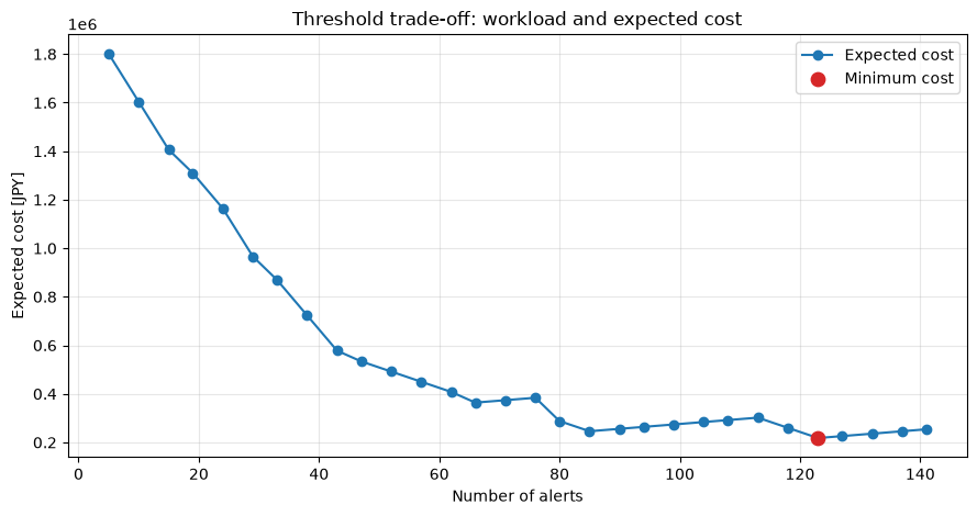 ### 結果の読み取り この仮定では、見逃し損失が誤検知コストより大きいため、アラートをある程度多く出す側が選ばれます。ただし最小コスト点が現場の点検上限を超える場合は、二段階判定や投票数で優先順位を付けます。費用係数を変えた感度分析も意思決定会議で提示します。 ## 対象ノックを通して見える実務上の示唆 1. **手法より先に意思決定を定義する**:出力を停止判断、点検候補、品質確認のどれに使うかで必要なRecallと説明粒度が変わります。 2. **異常率はモデルに与える前提**:5%抽出したから故障率が5%だとは言えません。点検能力と監査結果から更新します。 3. **複数手法の合意を監査に使う**:モデル投票は真実ではありませんが、初期のラベル収集を効率化できます。 4. **標準化と運転条件の分離が重要**:品種や設備が混在すると、単なる条件差を異常として検出します。 5. **スコアと根拠値を同時に見せる**:現場には順位だけでなく、どのセンサーが通常域から離れたかを提示します。 ## 実務導入する場合に必要なこと - 設備ID、品種、金型、立上げ・定常運転、保全履歴を分析単位に結合する - センサー欠測、張り付き、校正ずれをモデル前段で監視する - 時系列を保った検証期間を設け、未来情報の混入を防ぐ - アラートごとに「確認結果・原因・対応」を記録し、監査ラベルを蓄積する - アラート件数、確認率、見逃し、平均確認時間、分布変化を運用KPIにする - モデル・標準化器・特徴量定義・しきい値・変更理由を版管理する - 安全に関わる設備では、モデルを既存保護回路の代替にせず補助情報として使う ## まとめ No.051〜No.060では、孤立、局所密度、境界、共分散、近傍距離、クラスタ密度という異なる考え方から多変量異常を捉えました。実務では一つのモデルのスコアを盲信せず、監査ラベルで比較し、点検能力と損失構造に合わせてしきい値を調整することが重要です。小規模なPoCでは、候補抽出→現場確認→ラベル蓄積→再評価の短いサイクルから始めると、設備固有の「業務上の異常」に近づけます。 ## 法人向けのご相談 数理工房では、製造データの整理、異常検知PoC、評価設計、現場運用に合わせたアラート設計までご支援します。「データはあるが故障ラベルが少ない」「誤検知が多く運用が続かない」といった段階から、課題と意思決定を整理できます。 > 📩 **お問い合わせ**: [surikobo.co.jp/contact](https://surikobo.co.jp/contact) > まずはお気軽にご相談ください。