
100本ノック / マーケティングサイエンス / マーケティングサイエンス100本ノック
製造業の需要予測をS&OPへつなぐ実践Python|階層予測・在庫・生産計画
需要予測を「当てる」から「供給を決める」へ
製造業のS&OPをつなぐ実践10ノック(No.041〜No.050)
産業用ポンプメーカーの架空データを題材に、製品・地域・全社で整合する需要予測、精度評価、販促効果、因果推論、S&OP、在庫・生産計画、不確実性評価、モンテカルロ・シミュレーションまでを一つの意思決定プロセスとして扱います。
このNotebookの到達点は、予測値を作ることではありません。営業・生産・調達が、同じ前提とリスクを見ながら次の一手を決められる状態を作ることです。掲載する数値・会社・製品はすべて架空です。
[!NOTE] 本資料は、数理工房 (もしくは代表である和山個人) が過去に企業研修において使用した notebook を企業様の許可を得て再構成・編集のうえ公開しています。
掲載データはすべて架空のものであり、実在する企業・工場・数値とは一切関係ありません。
はじめに:この記事で扱う製造業の実務課題
受注生産と見込生産が混在する製造業では、「来月何台売れるか」だけでは意思決定できません。どの地域・製品で増減するのか、販促による上振れは一時的か、予測誤差に備えて何台持つか、限られた能力をどこへ配分するかまで結び付ける必要があります。
現場でよくある状況
- 営業は案件情報を上乗せし、生産は欠品回避のため多めに作り、経営は在庫圧縮を求める
- 全社予測と製品別予測を別々に作り、合計が一致しない
- MAPEだけでモデルを選び、過小予測・過大予測の経営上の非対称性を見落とす
- 販促期間の売上増をそのまま「効果」とみなし、季節性や市場変化を除けていない
- 点予測だけで計画し、需要変動・供給制約・欠品損失を会議で議論できない
なぜこの問題は判断が難しいのか
需要は、季節性、地域差、製品ライフサイクル、価格・販促、偶然変動が重なって観測されます。さらに、予測の目的関数と事業の目的関数は同じとは限りません。統計誤差が小さくても、利益率の高い製品を欠品させれば経営判断としては失敗です。本稿では、精度・整合性・因果・制約・不確実性の5点を同時に扱います。
今回扱うノックの全体像
| No. | テーマ | 意思決定への接続 |
|---|---|---|
| 041 | 階層時系列 | 全社・地域・製品の数字を一致させる |
| 042 | 予測精度評価 | 誤差を複数指標と偏りで評価する |
| 043 | プロモーション効果 | 売上の増分と採算を推定する |
| 044 | 因果推論と需要予測 | 自然増と施策効果を切り分ける |
| 045 | S&OP | 需要と供給能力のギャップを共有する |
| 046 | 在庫との連携 | サービス水準を安全在庫へ変換する |
| 047 | 生産計画との連携 | 能力制約下で限界利益を守る |
| 048 | 不確実性 | 点ではなく予測区間で判断する |
| 049 | 予測シミュレーション | 欠品・在庫・利益の分布を比較する |
| 050 | 実務事例 | KPIを統合して意思決定案を作る |
Python 環境の準備
外部データには依存せず、NumPy・pandas・matplotlibだけで再現します。乱数シードは固定します。
import sys
import numpy as np
import pandas as pd
import matplotlib
import matplotlib.pyplot as plt

SEED = 42
rng = np.random.default_rng(SEED)
pd.set_option("display.max_columns", 20)
pd.set_option("display.float_format", lambda x: f"{x:,.2f}")
plt.rcParams.update({"figure.figsize": (9, 4.5), "axes.unicode_minus": False})

print(f"Python     : {sys.version.split()[0]}")
print(f"NumPy      : {np.__version__}")
print(f"pandas     : {pd.__version__}")
print(f"matplotlib : {matplotlib.__version__}")
print(f"random seed: {SEED}")
Python : 3.13.1
NumPy : 2.5.1
pandas : 3.0.3
matplotlib : 3.11.0
random seed: 42架空データの作成
対象は産業用ポンプ3製品(Standard、EnergySaver、HeavyDuty)、3地域、104週です。トレンド、年周期、地域差、製品差、販促、ノイズから需要を生成します。東日本のEnergySaverには後半の販促を設定し、No.043〜044で効果を検証します。
weeks = pd.date_range("2024-01-01", periods=104, freq="W-MON")
products = ["Standard", "EnergySaver", "HeavyDuty"]
regions = ["East", "Central", "West"]
base = {"Standard": 82, "EnergySaver": 57, "HeavyDuty": 38}
product_margin = {"Standard": 48, "EnergySaver": 72, "HeavyDuty": 95}  # 千円/台
region_factor = {"East": 1.10, "Central": 0.88, "West": 1.00}

rows = []
for t, week in enumerate(weeks):
    season = 1 + 0.14 * np.sin(2 * np.pi * t / 52) + 0.05 * np.cos(4 * np.pi * t / 52)
    for region in regions:
        for product in products:
            promo = int(product == "EnergySaver" and region == "East" and 72 <= t <= 83)
            trend = 1 + (0.0018 if product == "EnergySaver" else 0.0005) * t
            latent = base[product] * region_factor[region] * season * trend + 16 * promo
            demand = max(0, int(round(latent + rng.normal(0, 7))))
            rows.append([week, t, region, product, promo, demand, latent])

df = pd.DataFrame(rows, columns=["week", "t", "region", "product", "promo", "demand", "latent_demand"])
print(f"rows={len(df):,}, weeks={df.week.nunique()}, products={df['product'].nunique()}, regions={df.region.nunique()}")
display(df.head(8))
rows=936, weeks=104, products=3, regions=3| week | t | region | product | promo | demand | latent_demand | |
|---|---|---|---|---|---|---|---|
| 0 | 2024-01-01 | 0 | East | Standard | 0 | 97 | 94.71 |
| 1 | 2024-01-01 | 0 | East | EnergySaver | 0 | 59 | 65.84 |
| 2 | 2024-01-01 | 0 | East | HeavyDuty | 0 | 49 | 43.89 |
| 3 | 2024-01-01 | 0 | Central | Standard | 0 | 82 | 75.77 |
| 4 | 2024-01-01 | 0 | Central | EnergySaver | 0 | 39 | 52.67 |
| 5 | 2024-01-01 | 0 | Central | HeavyDuty | 0 | 26 | 35.11 |
| 6 | 2024-01-01 | 0 | West | Standard | 0 | 87 | 86.10 |
| 7 | 2024-01-01 | 0 | West | EnergySaver | 0 | 58 | 59.85 |
weekly_total = df.groupby("week", as_index=False)["demand"].sum()
fig, ax = plt.subplots()
ax.plot(weekly_total["week"], weekly_total["demand"], color="#176B87", linewidth=1.8)
ax.set_title("Weekly total demand (synthetic industrial pumps)")
ax.set_xlabel("Week")
ax.set_ylabel("Units")
ax.grid(True, alpha=0.3)
fig.tight_layout()
plt.show()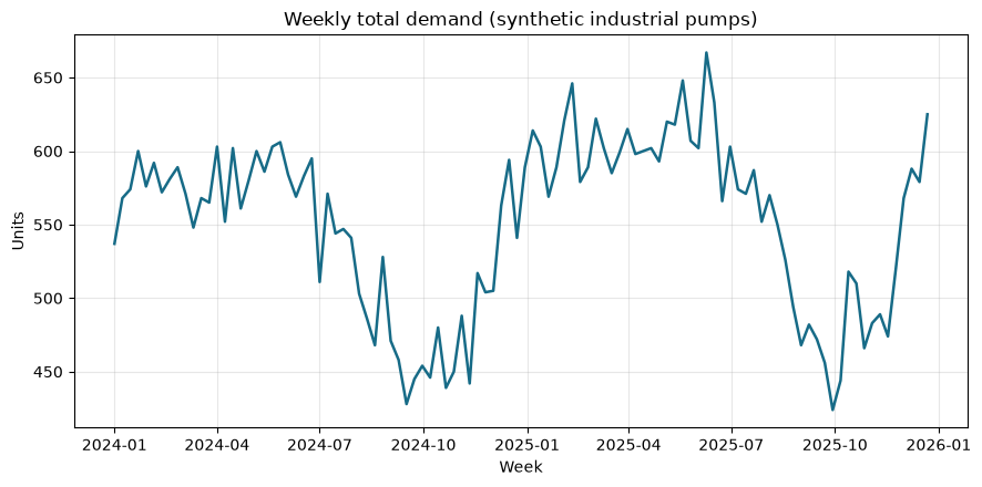
No.041:階層時系列 — 全社・地域・製品の予測を整合させる
実務での意味
経営会議は全社合計、営業は地域別、生産は製品別を見るため、各階層の予測が食い違うと同じ会社の中に複数の「正解」が生まれます。階層時系列では、最下層を合計するボトムアップ法などにより整合性を確保します。
分析・モデル化の考え方
最下層系列を とすると、全社予測は です。ここでは各地域×製品の直近8週平均を次週予測とし、地域・製品・全社へ集約します。高度な実務では、トップダウン法やMinT法も候補になります。
Pythonで確認する
cutoff = weeks[-1]
bottom_forecast = (df[df.week > cutoff - pd.Timedelta(weeks=8)]
                   .groupby(["region", "product"])["demand"].mean()
                   .rename("forecast").reset_index())
by_region = bottom_forecast.groupby("region")["forecast"].sum().rename("region_forecast")
by_product = bottom_forecast.groupby("product")["forecast"].sum().rename("product_forecast")
company = bottom_forecast["forecast"].sum()
display(bottom_forecast.pivot(index="region", columns="product", values="forecast").round(1))
print(f"Company forecast: {company:.1f} units")
print(f"Reconciliation check (region sum - company): {by_region.sum() - company:.10f}")| product | EnergySaver | HeavyDuty | Standard |
|---|---|---|---|
| region | |||
| Central | 57.00 | 35.40 | 72.80 |
| East | 65.50 | 37.80 | 89.00 |
| West | 64.10 | 38.20 | 81.00 |
Company forecast: 540.8 units
Reconciliation check (region sum - company): 0.0000000000
結果の読み取り
地域別・製品別のどちらから合計しても全社予測が一致します。重要なのはモデルの巧妙さより、会議資料・MRP・営業見通しが同じ集計構造を参照することです。ただし、最下層が疎な場合はボトムアップが不安定になるため、階層ごとの誤差共分散を使うMinTなどを検討します。
No.042:予測精度評価 — 平均誤差だけでモデルを選ばない
実務での意味
欠品と過剰在庫の損失は非対称です。したがって「平均的に何%外したか」に加え、継続的な過小予測がないかを確認する必要があります。
分析・モデル化の考え方
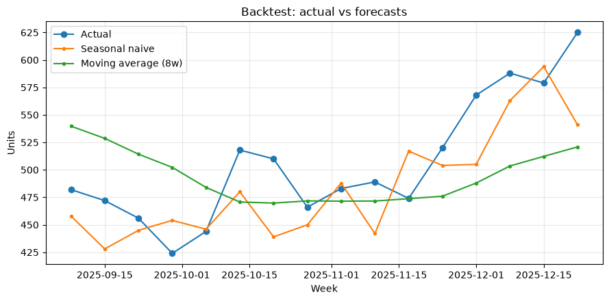
評価期間を最後の16週とし、ナイーブ予測(前年同週)と移動平均を比較します。MAE、RMSE、WAPEに加え、 を確認します。WAPEはゼロ需要を含む明細にも比較的扱いやすい一方、大需要系列の影響が強い指標です。
Pythonで確認する
total = weekly_total.set_index("week")["demand"]
actual = total.iloc[-16:]
pred_naive = total.shift(52).reindex(actual.index)
pred_ma8 = total.shift(1).rolling(8).mean().reindex(actual.index)

def metrics(y, pred):
    e = pred - y
    return {"MAE": np.abs(e).mean(), "RMSE": np.sqrt(np.mean(e**2)),
            "WAPE_%": 100*np.abs(e).sum()/y.sum(), "Bias_%": 100*e.sum()/y.sum()}

score = pd.DataFrame({"Seasonal naive": metrics(actual, pred_naive),
                      "Moving average (8w)": metrics(actual, pred_ma8)}).T
display(score.round(2))

fig, ax = plt.subplots()
ax.plot(actual.index, actual, marker="o", label="Actual")
ax.plot(actual.index, pred_naive, marker=".", label="Seasonal naive")
ax.plot(actual.index, pred_ma8, marker=".", label="Moving average (8w)")
ax.set_title("Backtest: actual vs forecasts")
ax.set_xlabel("Week"); ax.set_ylabel("Units"); ax.grid(True, alpha=0.3); ax.legend()
fig.tight_layout(); plt.show()| MAE | RMSE | WAPE_% | Bias_% | |
|---|---|---|---|---|
| Seasonal naive | 33.38 | 40.69 | 6.59 | -4.25 |
| Moving average (8w) | 49.54 | 57.42 | 9.79 | -2.46 |
結果の読み取り
RMSEは大きな外れを強く罰し、Biasは過大・過小の方向を示します。採用モデルは単一指標の最小値ではなく、「許容できる欠品リスクか」「誤差が特定時期に集中していないか」まで残差を確認して決めます。
No.043:プロモーション効果 — 増分需要と採算を測る
実務での意味
販促中の売上が高くても、季節要因や成長トレンドによる自然増なら販促費の成果ではありません。増分台数と限界利益を算出して、継続可否を判断します。
分析・モデル化の考え方
East×EnergySaverについて、販促直前12週の同曜日系列を基準とした簡易反実仮想を作ります。ここでは季節性の影響が近い短期間という前提です。増分利益は とします。
Pythonで確認する
target = df[(df.region == "East") & (df["product"] == "EnergySaver")].copy()
promo_rows = target[target.promo == 1]
pre = target[(target.t >= 60) & (target.t <= 71)]
baseline = pre.demand.mean()
incremental_units = promo_rows.demand.sum() - baseline * len(promo_rows)
campaign_cost = 620  # 千円
incremental_profit = incremental_units * product_margin["EnergySaver"] - campaign_cost
promo_result = pd.Series({"Baseline units/week": baseline,
                          "Promo units/week": promo_rows.demand.mean(),
                          "Incremental units": incremental_units,
                          "Campaign cost (kJPY)": campaign_cost,
                          "Incremental profit (kJPY)": incremental_profit})
display(promo_result.to_frame("estimate").round(1))| estimate | |
|---|---|
| Baseline units/week | 76.60 |
| Promo units/week | 90.50 |
| Incremental units | 167.00 |
| Campaign cost (kJPY) | 620.00 |
| Incremental profit (kJPY) | 11,404.00 |
結果の読み取り
販促期間と直前期間の差は「効果の初期推定」です。採算が正でも、前倒し購入や他地域からの需要移転があれば全社増分は小さくなります。次のノックで対照群を使い、共通変動を除きます。
No.044:因果推論と需要予測 — 施策がなかった世界と比較する
実務での意味
プロモーションの因果効果を需要予測に組み込めると、「通常需要」と「施策による上乗せ」を分けて生産へ渡せます。単純な前後比較より説明責任が高まります。
分析・モデル化の考え方
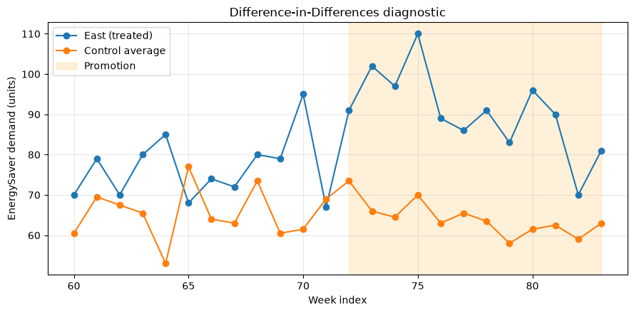
Eastを処置群、CentralとWestを対照群とする差の差(Difference-in-Differences)を用います。
重要な仮定は、施策がなければ群間のトレンドが平行だったことです。
Pythonで確認する
es = df[df["product"] == "EnergySaver"].copy()
es["period"] = np.where(es.t.between(72, 83), "post", "pre")
window = es[es.t.between(60, 83)].copy()
window["group"] = np.where(window.region == "East", "treated", "control")
means = window.groupby(["group", "period"])["demand"].mean().unstack()
did = (means.loc["treated", "post"] - means.loc["treated", "pre"]
       - means.loc["control", "post"] + means.loc["control", "pre"])
display(means.round(2))
print(f"Difference-in-Differences estimate: {did:.2f} units/week")

plot_did = window.groupby(["t", "group"])["demand"].mean().unstack()
fig, ax = plt.subplots()
ax.plot(plot_did.index, plot_did["treated"], marker="o", label="East (treated)")
ax.plot(plot_did.index, plot_did["control"], marker="o", label="Control average")
ax.axvspan(72, 83, alpha=0.15, color="orange", label="Promotion")
ax.set_title("Difference-in-Differences diagnostic")
ax.set_xlabel("Week index"); ax.set_ylabel("EnergySaver demand (units)")
ax.grid(True, alpha=0.3); ax.legend(); fig.tight_layout(); plt.show()| period | post | pre |
|---|---|---|
| group | ||
| control | 64.17 | 65.38 |
| treated | 90.50 | 76.58 |
Difference-in-Differences estimate: 15.12 units/week
結果の読み取り
差の差推定値は、対照群にも生じた市場変動を差し引いた週次増分です。導入前の線が概ね平行かをグラフで確認し、地域固有イベントや波及効果がある場合は設計を見直します。実運用では複数回の施策、価格、休日を含む回帰や実験設計へ拡張します。
No.045:S&OP — 需要計画と供給能力を同じ表にする
実務での意味
S&OP(Sales and Operations Planning)の中心は予測モデルではなく、需要・供給・財務を横断した合意形成です。能力不足を早期に可視化し、残業、外注、納期調整、販促変更を選べる時間を作ります。
分析・モデル化の考え方
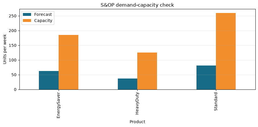
次の4週を製品別に予測し、通常能力との差を計算します。利用率 が100%を超える製品を例外管理の対象とします。
Pythonで確認する
recent = df[df.week > cutoff - pd.Timedelta(weeks=8)].groupby("product")["demand"].mean()
capacity = pd.Series({"Standard": 260, "EnergySaver": 185, "HeavyDuty": 125}, name="capacity_per_week")
sop = pd.concat([recent.rename("forecast_per_week"), capacity], axis=1)
sop["gap_units"] = sop.capacity_per_week - sop.forecast_per_week
sop["utilization_%"] = 100 * sop.forecast_per_week / sop.capacity_per_week
sop["status"] = np.where(sop["utilization_%"] > 100, "ACTION", np.where(sop["utilization_%"] > 90, "WATCH", "OK"))
display(sop.round(1))

fig, ax = plt.subplots()
sop[["forecast_per_week", "capacity_per_week"]].plot(kind="bar", ax=ax, color=["#176B87", "#F28E2B"])
ax.set_title("S&OP demand-capacity check")
ax.set_xlabel("Product"); ax.set_ylabel("Units per week"); ax.grid(True, axis="y", alpha=0.3)
ax.legend(["Forecast", "Capacity"]); fig.tight_layout(); plt.show()| forecast_per_week | capacity_per_week | gap_units | utilization_% | status | |
|---|---|---|---|---|---|
| EnergySaver | 62.20 | 185 | 122.80 | 33.60 | OK |
| HeavyDuty | 37.10 | 125 | 87.90 | 29.70 | OK |
| Standard | 80.90 | 260 | 179.10 | 31.10 | OK |
結果の読み取り
利用率の高い製品を会議の論点として絞り込めます。ここでのギャップは確定値ではなく、営業案件・設備停止・部材制約を加えてシナリオ更新する入口です。S&OPでは予測の版、前提、意思決定者、期限も記録します。
No.046:在庫との連携 — 予測誤差を安全在庫へ変換する
実務での意味
平均需要だけを補充すると、ばらつきの大きい製品ほど欠品します。一方、全品目に高いサービス水準を課すと在庫が膨らみます。重要度別の水準設計が必要です。
分析・モデル化の考え方
需要が独立でリードタイムが固定という簡易仮定のもと、安全在庫を 、発注点を とします。 は目標サービス水準に対応する係数です。
Pythonで確認する
stats = df.groupby("product")["demand"].agg(["mean", "std"])
lead_time = pd.Series({"Standard": 2, "EnergySaver": 3, "HeavyDuty": 4}, name="lead_weeks")
z = pd.Series({"Standard": 1.28, "EnergySaver": 1.65, "HeavyDuty": 2.05}, name="z_value")
inventory = stats.join(lead_time).join(z)
inventory["safety_stock"] = inventory.z_value * inventory["std"] * np.sqrt(inventory.lead_weeks)
inventory["reorder_point"] = inventory["mean"] * inventory.lead_weeks + inventory.safety_stock
display(inventory.round(1))| mean | std | lead_weeks | z_value | safety_stock | reorder_point | |
|---|---|---|---|---|---|---|
| product | ||||||
| EnergySaver | 62.00 | 11.90 | 3 | 1.60 | 33.90 | 219.90 |
| HeavyDuty | 38.50 | 8.50 | 4 | 2.00 | 35.00 | 188.80 |
| Standard | 83.40 | 13.00 | 2 | 1.30 | 23.60 | 190.30 |
結果の読み取り
リードタイム、需要変動、要求サービス水準のいずれかが高いほど安全在庫は増えます。式の前提が崩れる季節需要や供給遅延には、期間別分布やシミュレーションを使います。在庫額だけでなく、欠品時の顧客影響と代替可否でサービス水準を設計します。
No.047:生産計画との連携 — 能力制約下で利益を守る
実務での意味
需要合計が能力を超えるとき、全製品を一律に削ると高収益・重要顧客向けを失う可能性があります。制約資源1時間当たりの限界利益で配分案を作り、営業上の優先条件と合わせて判断します。
分析・モデル化の考え方
1週間の組立能力を1,350時間とし、まず最低供給量を確保したうえで、 の高い順に残余能力を割り当てる簡易ヒューリスティックを使います。これは説明可能な基準案であり、段取り・ロット・複数工程がある場合は整数計画法へ拡張します。
Pythonで確認する
plan = pd.DataFrame({
    "demand": sop.forecast_per_week.round(),
    "hours_per_unit": pd.Series({"Standard": 2.8, "EnergySaver": 3.6, "HeavyDuty": 5.2}),
    "margin_kJPY": pd.Series(product_margin),
    "minimum_supply": pd.Series({"Standard": 180, "EnergySaver": 125, "HeavyDuty": 75})
})
plan["margin_per_hour"] = plan.margin_kJPY / plan.hours_per_unit
plan["production"] = np.minimum(plan.demand, plan.minimum_supply)
hours_left = 1350 - (plan.production * plan.hours_per_unit).sum()
for product in plan.sort_values("margin_per_hour", ascending=False).index:
    add = min(plan.loc[product, "demand"] - plan.loc[product, "production"],
              np.floor(hours_left / plan.loc[product, "hours_per_unit"]))
    plan.loc[product, "production"] += max(0, add)
    hours_left -= max(0, add) * plan.loc[product, "hours_per_unit"]
plan["unmet_demand"] = plan.demand - plan.production
plan["expected_margin_kJPY"] = plan.production * plan.margin_kJPY
display(plan.round(1))
print(f"Remaining capacity: {hours_left:.1f} hours")| demand | hours_per_unit | margin_kJPY | minimum_supply | margin_per_hour | production | unmet_demand | expected_margin_kJPY | |
|---|---|---|---|---|---|---|---|---|
| EnergySaver | 62.00 | 3.60 | 72 | 125 | 20.00 | 62.00 | 0.00 | 4,464.00 |
| HeavyDuty | 37.00 | 5.20 | 95 | 75 | 18.30 | 37.00 | 0.00 | 3,515.00 |
| Standard | 81.00 | 2.80 | 48 | 180 | 17.10 | 81.00 | 0.00 | 3,888.00 |
Remaining capacity: 707.6 hours結果の読み取り
限界利益と最低供給を明示したため、配分の理由を説明できます。ただし、長期顧客価値、契約ペナルティ、市場シェアなど数値化しにくい条件もあります。最適化結果を自動決定ではなく、例外を議論する基準案として使うのが実務的です。
No.048:不確実性 — 予測区間でリスクを伝える
実務での意味
点予測が500台でも、480〜520台と300〜700台では計画の意味が異なります。予測区間は、経営に「どこまで外れ得るか」を伝える共通言語です。
分析・モデル化の考え方
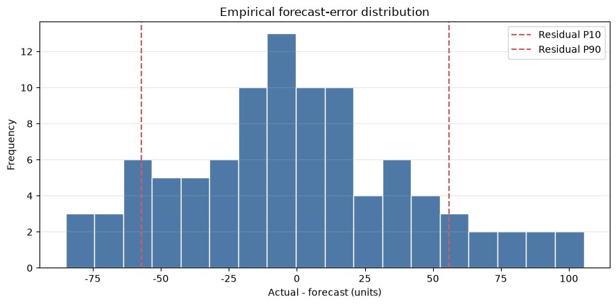
8週移動平均の1期先残差をバックテストし、経験分布の10%・90%点を点予測へ加えます。正規分布を仮定しない簡易な80%予測区間です。区間は将来の真値を必ず含む範囲ではなく、同じ手順を繰り返したときの被覆率を目標とします。
Pythonで確認する
ma_pred_all = total.shift(1).rolling(8).mean()
residuals = (total - ma_pred_all).dropna()
next_point = total.iloc[-8:].mean()
q10, q90 = residuals.quantile([0.10, 0.90])
interval = pd.Series({"P10": next_point + q10, "Point forecast": next_point, "P90": next_point + q90})
display(interval.to_frame("next_week_units").round(1))

fig, ax = plt.subplots()
ax.hist(residuals, bins=18, color="#4E79A7", edgecolor="white")
ax.axvline(q10, color="#E15759", linestyle="--", label="Residual P10")
ax.axvline(q90, color="#E15759", linestyle="--", label="Residual P90")
ax.set_title("Empirical forecast-error distribution")
ax.set_xlabel("Actual - forecast (units)"); ax.set_ylabel("Frequency")
ax.grid(True, axis="y", alpha=0.3); ax.legend(); fig.tight_layout(); plt.show()| next_week_units | |
|---|---|
| P10 | 483.70 |
| Point forecast | 540.80 |
| P90 | 596.60 |
結果の読み取り
P90近辺まで供給できる体制は欠品を減らしますが、在庫・残業コストを増やします。繁忙期と平常期で残差分布が違う場合は区間を分け、実績被覆率を継続監視します。区間幅が広い系列は、追加情報の収集価値が高い系列でもあります。
No.049:予測シミュレーション — 方針ごとの利益分布を比較する
実務での意味
平均ケースで優れた計画が、需要上振れ時に大きな機会損失を生むことがあります。シミュレーションにより、平均利益だけでなく下振れと欠品確率を比較できます。
分析・モデル化の考え方
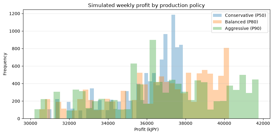
次週需要を残差の経験分布から10,000回生成し、保守的・標準・積極的の3生産方針を比較します。販売限界利益を70千円/台、余剰在庫費を12千円/台、欠品機会損失を28千円/台とする簡易損益です。
Pythonで確認する
sim_rng = np.random.default_rng(SEED + 1)
sim_demand = np.maximum(0, next_point + sim_rng.choice(residuals.to_numpy(), size=10_000, replace=True))
policies = {"Conservative (P50)": round(next_point),
            "Balanced (P80)": round(next_point + residuals.quantile(0.80)),
            "Aggressive (P90)": round(next_point + q90)}
records = []
profit_samples = {}
for name, qty in policies.items():
    sales = np.minimum(qty, sim_demand)
    leftover = np.maximum(qty - sim_demand, 0)
    shortage = np.maximum(sim_demand - qty, 0)
    profit = 70 * sales - 12 * leftover - 28 * shortage
    profit_samples[name] = profit
    records.append([name, qty, profit.mean(), np.quantile(profit, .10), (shortage > 0).mean()*100, leftover.mean()])
sim_result = pd.DataFrame(records, columns=["Policy", "Plan units", "Mean profit (kJPY)", "P10 profit (kJPY)", "Stockout probability (%)", "Mean leftover"])
display(sim_result.set_index("Policy").round(1))

fig, ax = plt.subplots()
for name, values in profit_samples.items():
    ax.hist(values, bins=35, alpha=0.35, label=name)
ax.set_title("Simulated weekly profit by production policy")
ax.set_xlabel("Profit (kJPY)"); ax.set_ylabel("Frequency")
ax.grid(True, axis="y", alpha=0.3); ax.legend(); fig.tight_layout(); plt.show()| Plan units | Mean profit (kJPY) | P10 profit (kJPY) | Stockout probability (%) | Mean leftover | |
|---|---|---|---|---|---|
| Policy | |||||
| Conservative (P50) | 541 | 35,989.20 | 33,134.50 | 44.40 | 17.40 |
| Balanced (P80) | 575 | 36,744.10 | 32,726.50 | 19.40 | 40.90 |
| Aggressive (P90) | 597 | 36,827.30 | 32,462.50 | 9.20 | 59.70 |
結果の読み取り
平均利益、P10利益、欠品確率、余剰在庫はトレードオフです。「最良」の方針は一意ではなく、会社のリスク許容度と顧客サービス方針で決まります。損失単価を関係部門と合意すると、感覚的な安全係数を経済価値に置き換えられます。
No.050:実務事例 — 予測から経営アクションまでを一本化する
実務での意味
分析が現場で使われるには、精度表だけで終わらず、「何を、誰が、いつ決めるか」へ翻訳する必要があります。本ノックでは、ここまでの結果を簡易S&OPスコアカードにまとめます。
分析・モデル化の考え方
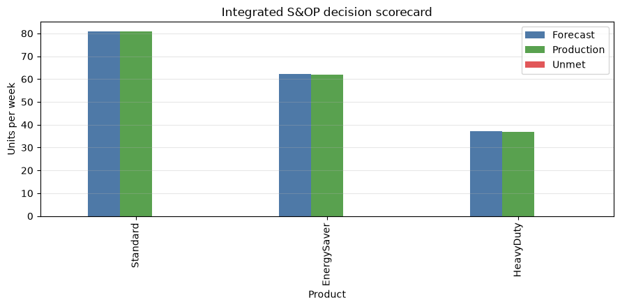
意思決定単位ごとに需要見通し、能力利用率、安全在庫、未充足需要、限界利益を並べます。KPIは局所最適を避けるため、サービス・在庫・能力・財務を同時に見ます。
Pythonで確認する
scorecard = pd.DataFrame(index=products)
scorecard["Forecast units/week"] = sop.forecast_per_week
scorecard["Capacity utilization %"] = sop["utilization_%"]
scorecard["Safety stock units"] = inventory.safety_stock
scorecard["Planned production"] = plan.production
scorecard["Unmet demand"] = plan.unmet_demand
scorecard["Margin kJPY/week"] = plan.expected_margin_kJPY
scorecard["Decision"] = [
    "Maintain; review excess capacity",
    "Protect supply; include promo uplift",
    "Prioritize key accounts; test overtime"
]
display(scorecard.round(1))

numeric = scorecard[["Forecast units/week", "Planned production", "Unmet demand"]]
fig, ax = plt.subplots()
numeric.plot(kind="bar", ax=ax, color=["#4E79A7", "#59A14F", "#E15759"])
ax.set_title("Integrated S&OP decision scorecard")
ax.set_xlabel("Product"); ax.set_ylabel("Units per week"); ax.grid(True, axis="y", alpha=0.3)
ax.legend(["Forecast", "Production", "Unmet"]); fig.tight_layout(); plt.show()| Forecast units/week | Capacity utilization % | Safety stock units | Planned production | Unmet demand | Margin kJPY/week | Decision | |
|---|---|---|---|---|---|---|---|
| Standard | 80.90 | 31.10 | 23.60 | 81.00 | 0.00 | 3,888.00 | Maintain; review excess capacity |
| EnergySaver | 62.20 | 33.60 | 33.90 | 62.00 | 0.00 | 4,464.00 | Protect supply; include promo uplift |
| HeavyDuty | 37.10 | 29.70 | 35.00 | 37.00 | 0.00 | 3,515.00 | Prioritize key accounts; test overtime |
結果の読み取り
スコアカードにより、予測の上振れ、供給能力、在庫、利益を同じ製品単位で議論できます。たとえばEnergySaverは販促増分を通常需要と分け、HeavyDutyは重要顧客と限界利益を考慮して能力追加を検討する、といった具体策へ落とせます。実務では各数値にデータ更新日、担当者、承認状態を付けます。
対象ノックを通して見える実務上の示唆
- 一つの数字より一つのプロセス:階層整合、精度、因果、供給制約を同じデータ更新サイクルに置くことが重要です。
- 予測誤差を経済価値へ翻訳する:WAPEの改善だけでなく、欠品損失・在庫費・限界利益で施策を評価します。
- 施策需要と基礎需要を分離する:販促上乗せを明示すると、営業施策と生産計画の責任範囲が見えます。
- 不確実性を隠さない:予測区間とシナリオを示すことで、残業・外注・在庫の保険料を議論できます。
- モデルは会議設計の一部:例外基準、意思決定期限、承認者まで定めて初めて成果につながります。
実務導入する場合に必要なこと
- 品目・顧客・地域・販促のマスタ統一と、受注・出荷・欠品の定義整理
- 時系列バックテスト、予測区間の被覆率、Biasの定期モニタリング
- 販促・価格変更・設備停止など「将来に既知の情報」の入力フロー
- 需要予測の版管理と、営業上書きの理由・効果を追跡する仕組み
- S&OP会議の粒度、頻度、例外閾値、決裁権限、KPIの明文化
- 予測精度だけでなく、在庫回転、納期遵守、欠品損失、利益への効果検証
まとめ
No.041〜050では、需要予測を階層整合から精度評価、販促の因果効果、S&OP、在庫・生産、不確実性、シミュレーションへ接続しました。高度なモデルを導入する前に、予測がどの意思決定を変えるのか、誤差を誰がどの費用で吸収するのかを定義することが成功の近道です。
法人向けのご相談
数理工房では、需要予測モデルの構築だけでなく、データ定義、精度評価、S&OP会議設計、在庫・生産最適化、現場で継続利用できる分析基盤まで、課題に応じてご支援します。
📩 お問い合わせ: surikobo.co.jp/contact
まずはお気軽にご相談ください。