From “Guessing” Demand Forecasting to “Determining Supply”

10 Practical Exercises Connecting S&OP in Manufacturing (No.041–No.050)

Using hypothetical data from industrial pump manufacturers as a subject, we handle a single decision-making process covering demand forecasting aligned across products, regions, and company-wide levels, including demand forecasting, accuracy evaluation, promotional effects, causal inference, S&OP, inventory and production planning, uncertainty assessment, and Monte Carlo simulation.

The goal of this notebook is not to create predictive values. It’s about creating Sales, production, and procurement can make their next move while considering the same assumptions and risks.. All figures, companies, and products listed are fictional.

[!NOTE] This material is a notebook previously used by Surikoubo (or personally by the representative, Kazuyama), and has been reconstructed, edited, and published with the company’s permission.
All data listed is fictional and has no relation whatsoever to real companies, factories, or figures.

Introduction: Practical Challenges in Manufacturing Covered in This Article

In manufacturing, where made-to-order and forecast-based production coexist, decisions cannot be made solely by “how many units will be sold next month.” It is necessary to link factors such as which regions and products will see increases or decreases, whether the upside from promotions is temporary, how many units to keep to prepare for forecast errors, and where to allocate limited capacity.

Common situations on site

• Sales add project information, production is increased to avoid stockouts, and management seeks inventory reduction.
• Company-wide forecasts and product-specific forecasts are created separately, resulting in inconsistent totals.
• Choosing models solely with MAPE and overestimating management asymmetries such as under-forecasting and overforecasting
• Treating sales increases during promotional periods as ‘effect’ without excluding seasonality or market changes.
• Planning is based solely on point forecasts, and it is impossible to discuss demand fluctuations, supply constraints, and shortage losses in meetings.

Why is this issue so difficult to judge?

Demand is observed through a combination of seasonality, regional differences, product life cycles, pricing and promotions, and random fluctuations. Furthermore, the objective function for forecasting and the objective function for business are not necessarily the same. Even if the statistical error is small, if you miss a product with a high profit margin, it is a failed management decision. This article addresses five Accuracy, Integrity, Causality, Constraints, Uncertainty points simultaneously.

Overview of Exercise covered this time

No.	Theme	Connecting to decision-making
041	hierarchical time series	Matching company-wide, regional, and product figures
042	Prediction accuracy evaluation	Evaluating errors using multiple indicators and biases
043	Promotional Effects	Estimating incremental sales and profitability
044	Causal Inference and Demand Forecasting	Distinguishing organic growth from policy effectiveness
045	S&OP	Sharing the gap between demand and supply capacity
046	Integration with Inventory	Converting service levels into safety stock
047	Coordination with Production Planning	Protecting marginal profits under capability constraints
048	uncertainty	Judge by the predicted interval, not the point
049	Predictive Simulation	Compare the distribution of stockouts, inventory, and profits
050	Practical Examples	Integrate KPIs to create decision-making proposals

Preparing the Python environment

It does not depend on external data; it reproduces using only NumPy, pandas, and matplotlib. Random number seeds are fixed.

import sys
import numpy as np
import pandas as pd
import matplotlib
import matplotlib.pyplot as plt

SEED = 42
rng = np.random.default_rng(SEED)
pd.set_option("display.max_columns", 20)
pd.set_option("display.float_format", lambda x: f"{x:,.2f}")
plt.rcParams.update({"figure.figsize": (9, 4.5), "axes.unicode_minus": False})

print(f"Python     : {sys.version.split()[0]}")
print(f"NumPy      : {np.__version__}")
print(f"pandas     : {pd.__version__}")
print(f"matplotlib : {matplotlib.__version__}")
print(f"random seed: {SEED}")

Python     : 3.13.1
NumPy      : 2.5.1
pandas     : 3.0.3
matplotlib : 3.11.0
random seed: 42

Creation of Fictional Data

The target is three industrial pump products (Standard, EnergySaver, HeavyDuty), covering three regions and 104 weeks. Demand is generated from trends, annual cycles, regional differences, product differences, promotions, and noise. We set up a promotional campaign for the latter half of the promotion at EnergySaver in eastern Japan, and verify its effectiveness in No.043–044.

weeks = pd.date_range("2024-01-01", periods=104, freq="W-MON")
products = ["Standard", "EnergySaver", "HeavyDuty"]
regions = ["East", "Central", "West"]
base = {"Standard": 82, "EnergySaver": 57, "HeavyDuty": 38}
product_margin = {"Standard": 48, "EnergySaver": 72, "HeavyDuty": 95}  # 1,000 yen per vehicle
region_factor = {"East": 1.10, "Central": 0.88, "West": 1.00}

rows = []
for t, week in enumerate(weeks):
    season = 1 + 0.14 * np.sin(2 * np.pi * t / 52) + 0.05 * np.cos(4 * np.pi * t / 52)
    for region in regions:
        for product in products:
            promo = int(product == "EnergySaver" and region == "East" and 72 <= t <= 83)
            trend = 1 + (0.0018 if product == "EnergySaver" else 0.0005) * t
            latent = base[product] * region_factor[region] * season * trend + 16 * promo
            demand = max(0, int(round(latent + rng.normal(0, 7))))
            rows.append([week, t, region, product, promo, demand, latent])

df = pd.DataFrame(rows, columns=["week", "t", "region", "product", "promo", "demand", "latent_demand"])
print(f"rows={len(df):,}, weeks={df.week.nunique()}, products={df['product'].nunique()}, regions={df.region.nunique()}")
display(df.head(8))

rows=936, weeks=104, products=3, regions=3

	week	t	region	product	promo	demand	latent_demand
0	2024-01-01	0	East	Standard	0	97	94.71
1	2024-01-01	0	East	EnergySaver	0	59	65.84
2	2024-01-01	0	East	HeavyDuty	0	49	43.89
3	2024-01-01	0	Central	Standard	0	82	75.77
4	2024-01-01	0	Central	EnergySaver	0	39	52.67
5	2024-01-01	0	Central	HeavyDuty	0	26	35.11
6	2024-01-01	0	West	Standard	0	87	86.10
7	2024-01-01	0	West	EnergySaver	0	58	59.85

weekly_total = df.groupby("week", as_index=False)["demand"].sum()
fig, ax = plt.subplots()
ax.plot(weekly_total["week"], weekly_total["demand"], color="#176B87", linewidth=1.8)
ax.set_title("Weekly total demand (synthetic industrial pumps)")
ax.set_xlabel("Week")
ax.set_ylabel("Units")
ax.grid(True, alpha=0.3)
fig.tight_layout()
plt.show()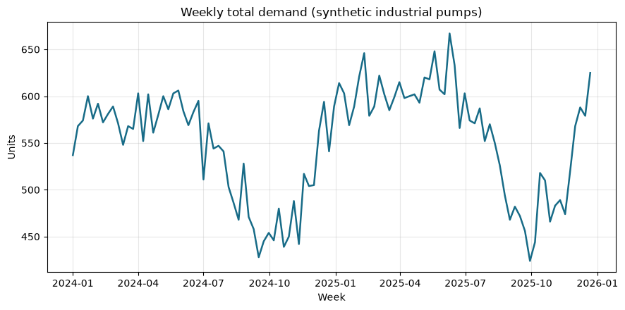

No.041: Hierarchical Time Series — Aligning Company-Wide, Regional, and Product Forecasts

Meaning in Practice

Management meetings look at the entire company, sales by region, and production by product, so when forecasts differ at each level, multiple “correct answers” emerge within the same company. In hierarchical chronological order, consistency is ensured through bottom-up methods such as summing the lowest layers.

Approach to Analysis and Modeling

If the bottom-tier group is $\hat{y}_{r,p,t}$, the company-wide forecast is $\hat{y}_{t}=\sum_r\sum_p\hat{y}_{r,p,t}$. Here, we use the most recent 8-week average for products × each region as the forecast for the next week and consolidate it across regions, products, and the entire company. In advanced practice, top-down and Mint methods are also candidates.

Check with Python

cutoff = weeks[-1]
bottom_forecast = (df[df.week > cutoff - pd.Timedelta(weeks=8)]
                   .groupby(["region", "product"])["demand"].mean()
                   .rename("forecast").reset_index())
by_region = bottom_forecast.groupby("region")["forecast"].sum().rename("region_forecast")
by_product = bottom_forecast.groupby("product")["forecast"].sum().rename("product_forecast")
company = bottom_forecast["forecast"].sum()
display(bottom_forecast.pivot(index="region", columns="product", values="forecast").round(1))
print(f"Company forecast: {company:.1f} units")
print(f"Reconciliation check (region sum - company): {by_region.sum() - company:.10f}")

product	EnergySaver	HeavyDuty	Standard
region
Central	57.00	35.40	72.80
East	65.50	37.80	89.00
West	64.10	38.20	81.00

Company forecast: 540.8 units
Reconciliation check (region sum - company): 0.0000000000

Reading the results

Whether you add up by region or product, the company-wide forecast is consistent. What matters more is not the cleverness of the model, but that meeting materials, MRPs, and sales outlooks all refer to the same aggregation structure. However, if the lowest layer is sparse, bottom-up becomes unstable, so consider methods such as MinT, which uses the covariance of error differences by layer.

No.042: Prediction accuracy evaluation — Choosing models based solely on average error

Meaning in Practice

Losses from stockouts and excess inventory are asymmetrical. Therefore, in addition to “what percentage was deviated on average,” it is necessary to check whether there is ongoing underforecasting.

Approach to Analysis and Modeling

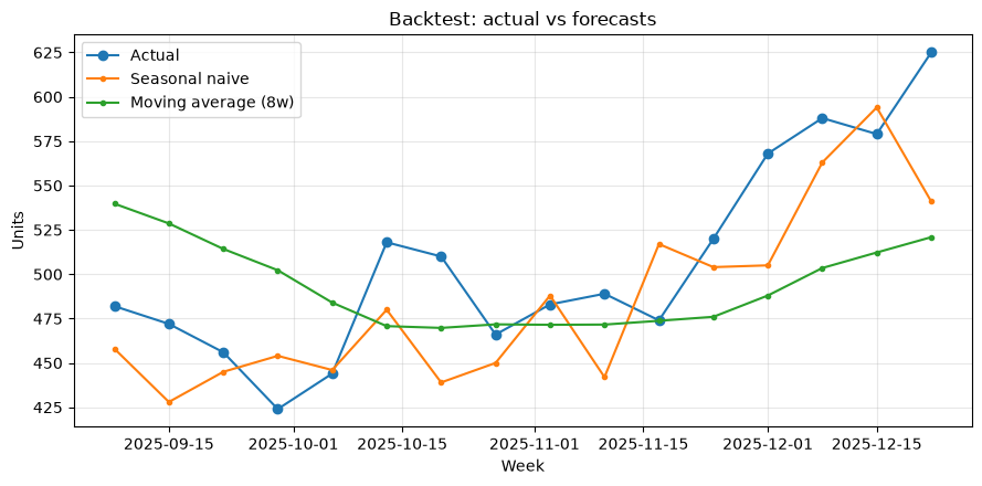
The evaluation period is the last 16 weeks, and naive forecasts (same week last year) are compared with moving averages. In addition to MAE, RMSE, and WAPE, we check $Bias=\sum(\hat{y}-y)/\sum y$. WAPE is relatively easy to handle even for items with zero demand, but is strongly influenced by large demand groups.

Check with Python

total = weekly_total.set_index("week")["demand"]
actual = total.iloc[-16:]
pred_naive = total.shift(52).reindex(actual.index)
pred_ma8 = total.shift(1).rolling(8).mean().reindex(actual.index)

def metrics(y, pred):
    e = pred - y
    return {"MAE": np.abs(e).mean(), "RMSE": np.sqrt(np.mean(e**2)),
            "WAPE_%": 100*np.abs(e).sum()/y.sum(), "Bias_%": 100*e.sum()/y.sum()}

score = pd.DataFrame({"Seasonal naive": metrics(actual, pred_naive),
                      "Moving average (8w)": metrics(actual, pred_ma8)}).T
display(score.round(2))

fig, ax = plt.subplots()
ax.plot(actual.index, actual, marker="o", label="Actual")
ax.plot(actual.index, pred_naive, marker=".", label="Seasonal naive")
ax.plot(actual.index, pred_ma8, marker=".", label="Moving average (8w)")
ax.set_title("Backtest: actual vs forecasts")
ax.set_xlabel("Week"); ax.set_ylabel("Units"); ax.grid(True, alpha=0.3); ax.legend()
fig.tight_layout(); plt.show()

	MAE	RMSE	WAPE_%	Bias_%
Seasonal naive	33.38	40.69	6.59	-4.25
Moving average (8w)	49.54	57.42	9.79	-2.46

Reading the results

RMSE strongly punishes large deviations, while Bias indicates over-the-under-the-top or under-the-limit directions. The adoption model does not determine the minimum value of a single metric, but also checks the residuals to determine whether the “acceptable out-of-stock risk” and “whether the error is concentrated at a specific time.”

No.043: Promotion Effect — Measuring Incremental Demand and Profitability

Meaning in Practice

Even if sales during promotions are high, if sales naturally increase due to seasonal factors or growth trends, it is not the result of promotional expenses. We calculate the incremental number of units and the marginal profit to determine whether continuation is possible.

Approach to Analysis and Modeling

Regarding East×EnergySaver, we create a simple counterfactual virtual based on the weekday series in the 12 weeks just before the promotion. Here, we assume the seasonal effects are short-term and close. Let the incremental profit be $\text{incremental units}\times\text{margin}-\text{campaign cost}$.

Check with Python

target = df[(df.region == "East") & (df["product"] == "EnergySaver")].copy()
promo_rows = target[target.promo == 1]
pre = target[(target.t >= 60) & (target.t <= 71)]
baseline = pre.demand.mean()
incremental_units = promo_rows.demand.sum() - baseline * len(promo_rows)
campaign_cost = 620  # thousand yen
incremental_profit = incremental_units * product_margin["EnergySaver"] - campaign_cost
promo_result = pd.Series({"Baseline units/week": baseline,
                          "Promo units/week": promo_rows.demand.mean(),
                          "Incremental units": incremental_units,
                          "Campaign cost (kJPY)": campaign_cost,
                          "Incremental profit (kJPY)": incremental_profit})
display(promo_result.to_frame("estimate").round(1))

	estimate
Baseline units/week	76.60
Promo units/week	90.50
Incremental units	167.00
Campaign cost (kJPY)	620.00
Incremental profit (kJPY)	11,404.00

Reading the results

The difference between the promotional period and the period just before is an “initial estimate of effectiveness.” Even if profitability is positive, if purchases are made earlier or demand shifts from other regions, the company-wide increment will be smaller. Use the control group for the next exercise and exclude common variation.

No.044: Causal Inference and Demand Forecasting — Comparing with a World Without Measures

Meaning in Practice

If you incorporate the causal effects of promotions into demand forecasting, you can separate “regular demand” from “additional incentives from measures” and pass them on to production. Accountability is greater than simple comparisons.

Approach to Analysis and Modeling

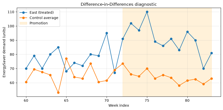
Difference-in-Differences are used, with East as the treatment group and Central and West as the control group.

$\widehat{ATE}=(\bar{Y}_{T,post}-\bar{Y}_{T,pre})-(\bar{Y}_{C,post}-\bar{Y}_{C,pre})$

An important assumption is that without measures, trends between groups were parallel.

Check with Python

es = df[df["product"] == "EnergySaver"].copy()
es["period"] = np.where(es.t.between(72, 83), "post", "pre")
window = es[es.t.between(60, 83)].copy()
window["group"] = np.where(window.region == "East", "treated", "control")
means = window.groupby(["group", "period"])["demand"].mean().unstack()
did = (means.loc["treated", "post"] - means.loc["treated", "pre"]
       - means.loc["control", "post"] + means.loc["control", "pre"])
display(means.round(2))
print(f"Difference-in-Differences estimate: {did:.2f} units/week")

plot_did = window.groupby(["t", "group"])["demand"].mean().unstack()
fig, ax = plt.subplots()
ax.plot(plot_did.index, plot_did["treated"], marker="o", label="East (treated)")
ax.plot(plot_did.index, plot_did["control"], marker="o", label="Control average")
ax.axvspan(72, 83, alpha=0.15, color="orange", label="Promotion")
ax.set_title("Difference-in-Differences diagnostic")
ax.set_xlabel("Week index"); ax.set_ylabel("EnergySaver demand (units)")
ax.grid(True, alpha=0.3); ax.legend(); fig.tight_layout(); plt.show()

period	post	pre
group
control	64.17	65.38
treated	90.50	76.58

Difference-in-Differences estimate: 15.12 units/week

Reading the results

The estimated difference is the weekly increment after subtracting market fluctuations that occurred in the control group. Check with graphs whether the lines before implementation are generally parallel, and review the design if there are region-specific events or ripple effects. In practice, it expands to include multiple rounds of measures, pricing, and holidays, including regression and experimental design.

No.045: S&OP — Putting demand planning and supply capacity in the same table

Meaning in Practice

At the heart of S&OP (Sales and Operations Planning) is not a forecasting model, but rather consensus building across demand, supply, and finance. We visualize shortcomings early and create time to choose overtime, outsourcing, delivery date adjustments, and promotional changes.

Approach to Analysis and Modeling

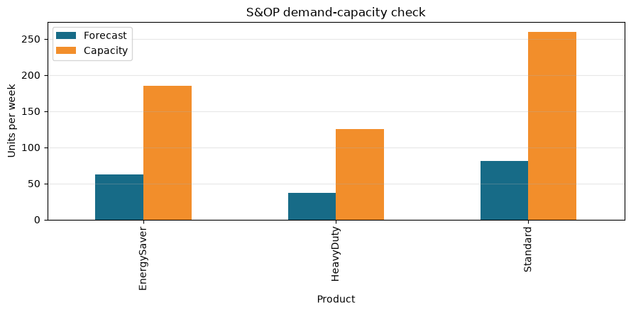
Forecast the next four weeks by product and calculate the difference from normal capacity. Products with a usage rate of $=need/Ability$ exceeding 100% are subject to exception management.

Check with Python

recent = df[df.week > cutoff - pd.Timedelta(weeks=8)].groupby("product")["demand"].mean()
capacity = pd.Series({"Standard": 260, "EnergySaver": 185, "HeavyDuty": 125}, name="capacity_per_week")
sop = pd.concat([recent.rename("forecast_per_week"), capacity], axis=1)
sop["gap_units"] = sop.capacity_per_week - sop.forecast_per_week
sop["utilization_%"] = 100 * sop.forecast_per_week / sop.capacity_per_week
sop["status"] = np.where(sop["utilization_%"] > 100, "ACTION", np.where(sop["utilization_%"] > 90, "WATCH", "OK"))
display(sop.round(1))

fig, ax = plt.subplots()
sop[["forecast_per_week", "capacity_per_week"]].plot(kind="bar", ax=ax, color=["#176B87", "#F28E2B"])
ax.set_title("S&OP demand-capacity check")
ax.set_xlabel("Product"); ax.set_ylabel("Units per week"); ax.grid(True, axis="y", alpha=0.3)
ax.legend(["Forecast", "Capacity"]); fig.tight_layout(); plt.show()

	forecast_per_week	capacity_per_week	gap_units	utilization_%	status
EnergySaver	62.20	185	122.80	33.60	OK
HeavyDuty	37.10	125	87.90	29.70	OK
Standard	80.90	260	179.10	31.10	OK

Reading the results

You can narrow down high-usage products as key points for meetings. The gap here is not a fixed value, but rather the entry point for scenario updates by adding sales projects, equipment stoppages, and material constraints. S&OP records forecasts, assumptions, decision-makers, and deadlines.

No.046: Collaboration with Inventory — Converting Forecast Errors into Safety Stock

Meaning in Practice

If you only replenish average demand, products with greater variability will be out of stock. On the other hand, imposing high service standards on all items will cause inventory to balloon. Level design is required according to importance.

Approach to Analysis and Modeling

Based on the simple assumption that demand is independent and lead time is fixed, safety stock is $SS=z\sigma\sqrt{L}$ and order points are $ROP=\mu L+SS$. $z$ is a coefficient corresponding to the target service level.

Check with Python

stats = df.groupby("product")["demand"].agg(["mean", "std"])
lead_time = pd.Series({"Standard": 2, "EnergySaver": 3, "HeavyDuty": 4}, name="lead_weeks")
z = pd.Series({"Standard": 1.28, "EnergySaver": 1.65, "HeavyDuty": 2.05}, name="z_value")
inventory = stats.join(lead_time).join(z)
inventory["safety_stock"] = inventory.z_value * inventory["std"] * np.sqrt(inventory.lead_weeks)
inventory["reorder_point"] = inventory["mean"] * inventory.lead_weeks + inventory.safety_stock
display(inventory.round(1))

	mean	std	lead_weeks	z_value	safety_stock	reorder_point
product
EnergySaver	62.00	11.90	3	1.60	33.90	219.90
HeavyDuty	38.50	8.50	4	2.00	35.00	188.80
Standard	83.40	13.00	2	1.30	23.60	190.30

Reading the results

The higher the lead time, demand fluctuations, or required service levels, the more safety stock increases. For seasonal demand and supply delays where the formula’s premise is broken, periodic distribution and simulations are used. We design service levels not only based on inventory levels but also on customer impact and substitution availability during out-of-stock situations.

No.047: Coordination with Production Planning — Protecting Profits Under Capacity Constraints

Meaning in Practice

When total demand exceeds capacity, cutting all products uniformly may result in losing high-profit, key customers. We create allocation plans based on marginal profit per hour of constrained resources and make decisions based on business priority conditions.

Approach to Analysis and Modeling

A simple heuristic, which assigns a weekly assembly capacity of 1,350 hours, securing a minimum supply and assigning remaining capacity in order of highest $\text{margin}/\text{hours}$. This is a describable standard draft, and if there are arrangements, lots, or multiple steps, it can be extended to integer programming.

Check with Python

plan = pd.DataFrame({
    "demand": sop.forecast_per_week.round(),
    "hours_per_unit": pd.Series({"Standard": 2.8, "EnergySaver": 3.6, "HeavyDuty": 5.2}),
    "margin_kJPY": pd.Series(product_margin),
    "minimum_supply": pd.Series({"Standard": 180, "EnergySaver": 125, "HeavyDuty": 75})
})
plan["margin_per_hour"] = plan.margin_kJPY / plan.hours_per_unit
plan["production"] = np.minimum(plan.demand, plan.minimum_supply)
hours_left = 1350 - (plan.production * plan.hours_per_unit).sum()
for product in plan.sort_values("margin_per_hour", ascending=False).index:
    add = min(plan.loc[product, "demand"] - plan.loc[product, "production"],
              np.floor(hours_left / plan.loc[product, "hours_per_unit"]))
    plan.loc[product, "production"] += max(0, add)
    hours_left -= max(0, add) * plan.loc[product, "hours_per_unit"]
plan["unmet_demand"] = plan.demand - plan.production
plan["expected_margin_kJPY"] = plan.production * plan.margin_kJPY
display(plan.round(1))
print(f"Remaining capacity: {hours_left:.1f} hours")

	demand	hours_per_unit	margin_kJPY	minimum_supply	margin_per_hour	production	unmet_demand	expected_margin_kJPY
EnergySaver	62.00	3.60	72	125	20.00	62.00	0.00	4,464.00
HeavyDuty	37.00	5.20	95	75	18.30	37.00	0.00	3,515.00
Standard	81.00	2.80	48	180	17.10	81.00	0.00	3,888.00

Remaining capacity: 707.6 hours

Reading the results

Since marginal profit and minimum supply are clearly stated, the reason for the allocation can be explained. However, there are also hard-to-quantify conditions such as long-term customer value, contract penalties, and market share. Practically, it is practical to use optimization results not as automated decisions, but as a benchmark for discussing exceptions.

No.048: Uncertainty — Communicating Risk in Forecast Intervals

Meaning in Practice

Even if the point forecast is 500 units, the meaning of the plan differs between 480–520 and 300–700 units. Forecast intervals are a common language that communicates to management about “how far we might deviate.”

Approach to Analysis and Modeling

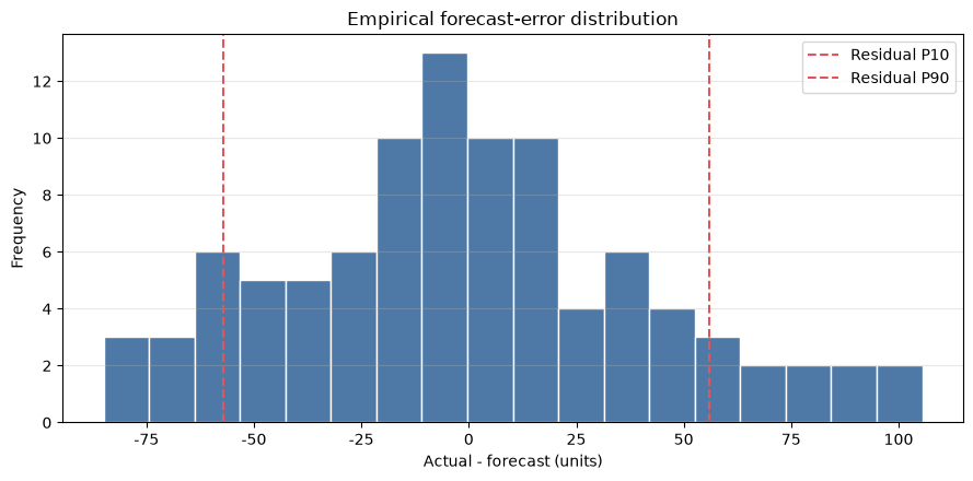
Backtest the one-term residual of the 8-week moving average, and add 10% and 90% of the experience distribution points to the point prediction. This is a simple 80% prediction interval that does not assume a normal distribution. The interval does not necessarily include future true values, but targets the coverage rate when repeating the same procedure.

Check with Python

ma_pred_all = total.shift(1).rolling(8).mean()
residuals = (total - ma_pred_all).dropna()
next_point = total.iloc[-8:].mean()
q10, q90 = residuals.quantile([0.10, 0.90])
interval = pd.Series({"P10": next_point + q10, "Point forecast": next_point, "P90": next_point + q90})
display(interval.to_frame("next_week_units").round(1))

fig, ax = plt.subplots()
ax.hist(residuals, bins=18, color="#4E79A7", edgecolor="white")
ax.axvline(q10, color="#E15759", linestyle="--", label="Residual P10")
ax.axvline(q90, color="#E15759", linestyle="--", label="Residual P90")
ax.set_title("Empirical forecast-error distribution")
ax.set_xlabel("Actual - forecast (units)"); ax.set_ylabel("Frequency")
ax.grid(True, axis="y", alpha=0.3); ax.legend(); fig.tight_layout(); plt.show()

	next_week_units
P10	483.70
Point forecast	540.80
P90	596.60

Reading the results

A system that can supply up to around P90 reduces shortages but increases inventory and overtime costs. If the residual distribution differs between busy and normal periods, the sections are separated and the actual coverage rate is continuously monitored. Networks with wide sections also have a high value for collecting additional information.

No.049: Forecast Simulation — Comparing Profit Distribution by Policy

Meaning in Practice

On average, a good plan can result in significant opportunity losses during demand downturns. Simulations allow comparison not only of average profits but also of downside and out-of-stock probabilities.

Approach to Analysis and Modeling

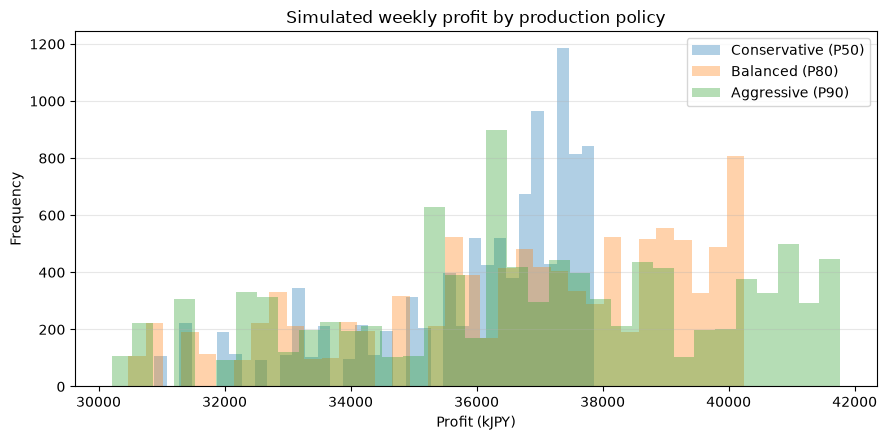
Next week’s demand is generated 10,000 times from the residual experience distribution, and three production policies are compared: conservative, standard, and aggressive. The simple profit and loss is 70,000 yen per unit based on marginal sales, 12,000 yen per unit of surplus inventory, and 28,000 yen per unit of out-of-stock opportunity loss.

Check with Python

sim_rng = np.random.default_rng(SEED + 1)
sim_demand = np.maximum(0, next_point + sim_rng.choice(residuals.to_numpy(), size=10_000, replace=True))
policies = {"Conservative (P50)": round(next_point),
            "Balanced (P80)": round(next_point + residuals.quantile(0.80)),
            "Aggressive (P90)": round(next_point + q90)}
records = []
profit_samples = {}
for name, qty in policies.items():
    sales = np.minimum(qty, sim_demand)
    leftover = np.maximum(qty - sim_demand, 0)
    shortage = np.maximum(sim_demand - qty, 0)
    profit = 70 * sales - 12 * leftover - 28 * shortage
    profit_samples[name] = profit
    records.append([name, qty, profit.mean(), np.quantile(profit, .10), (shortage > 0).mean()*100, leftover.mean()])
sim_result = pd.DataFrame(records, columns=["Policy", "Plan units", "Mean profit (kJPY)", "P10 profit (kJPY)", "Stockout probability (%)", "Mean leftover"])
display(sim_result.set_index("Policy").round(1))

fig, ax = plt.subplots()
for name, values in profit_samples.items():
    ax.hist(values, bins=35, alpha=0.35, label=name)
ax.set_title("Simulated weekly profit by production policy")
ax.set_xlabel("Profit (kJPY)"); ax.set_ylabel("Frequency")
ax.grid(True, axis="y", alpha=0.3); ax.legend(); fig.tight_layout(); plt.show()

	Plan units	Mean profit (kJPY)	P10 profit (kJPY)	Stockout probability (%)	Mean leftover
Policy
Conservative (P50)	541	35,989.20	33,134.50	44.40	17.40
Balanced (P80)	575	36,744.10	32,726.50	19.40	40.90
Aggressive (P90)	597	36,827.30	32,462.50	9.20	59.70

Reading the results

Average profit, P10 profit, out-of-stock probability, and surplus inventory are trade-offs. The “best” policy is not unique; it is determined by the company’s risk tolerance and customer service policies. When the unit price of loss is agreed upon with relevant departments, the perceived safety factor is replaced by economic value.

No.050: Practical Case Study — Unifying Forecasting from Management Actions

Meaning in Practice

For analysis to be used in the field, it is necessary to translate beyond just accuracy sheets into “what, who, and when to decide.” In this exercise, we will summarize the results so far into a simplified S&OP scorecard.

Approach to Analysis and Modeling

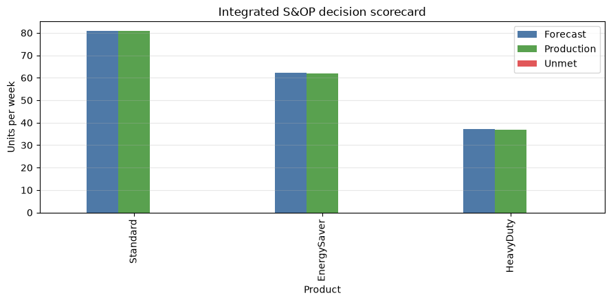
For each decision-making unit, we list demand outlooks, capacity utilization, safety stock, unmet demand, and marginal profit. To avoid local optimization, KPIs simultaneously look at service, inventory, capability, and finance.

Check with Python

scorecard = pd.DataFrame(index=products)
scorecard["Forecast units/week"] = sop.forecast_per_week
scorecard["Capacity utilization %"] = sop["utilization_%"]
scorecard["Safety stock units"] = inventory.safety_stock
scorecard["Planned production"] = plan.production
scorecard["Unmet demand"] = plan.unmet_demand
scorecard["Margin kJPY/week"] = plan.expected_margin_kJPY
scorecard["Decision"] = [
    "Maintain; review excess capacity",
    "Protect supply; include promo uplift",
    "Prioritize key accounts; test overtime"
]
display(scorecard.round(1))

numeric = scorecard[["Forecast units/week", "Planned production", "Unmet demand"]]
fig, ax = plt.subplots()
numeric.plot(kind="bar", ax=ax, color=["#4E79A7", "#59A14F", "#E15759"])
ax.set_title("Integrated S&OP decision scorecard")
ax.set_xlabel("Product"); ax.set_ylabel("Units per week"); ax.grid(True, axis="y", alpha=0.3)
ax.legend(["Forecast", "Production", "Unmet"]); fig.tight_layout(); plt.show()

	Forecast units/week	Capacity utilization %	Safety stock units	Planned production	Unmet demand	Margin kJPY/week	Decision
Standard	80.90	31.10	23.60	81.00	0.00	3,888.00	Maintain; review excess capacity
EnergySaver	62.20	33.60	33.90	62.00	0.00	4,464.00	Protect supply; include promo uplift
HeavyDuty	37.10	29.70	35.00	37.00	0.00	3,515.00	Prioritize key accounts; test overtime

Reading the results

The scorecard allows you to discuss forecasts, supply capacity, inventory, and profits within the same product unit. For example, EnergySaver can separate promotional increments from regular demand, while HeavyDuty can consider adding capacity based on key customers and marginal profits, among other concrete measures. In practice, each value is marked with the data update date, person in charge, and approval status.

Practical Implications Seen Through Target Exercise

1. One process is better than one number: It is important to place hierarchical consistency, accuracy, causality, and supply constraints in the same data update cycle.
2. Translating forecast errors into economic value: Evaluate measures not only by WAPE improvements but also by out-of-stock losses, inventory costs, and marginal profit.
3. Separating policy demand from basic demand: Clearly indicating promotional surcharges reveals the scope of responsibility for sales strategies and production planning.
4. Don’t hide uncertainty: By showing forecast intervals and scenarios, you can discuss insurance premiums for overtime, outsourcing, and inventory.
5. The model is part of meeting design.: Only when exception criteria, decision-making deadlines, and approvers are set can results be achieved.

What is necessary for practical implementation

• Unifying master systems for items, customers, regions, and promotions, and organizing definitions of orders, shipments, and out-of-stock items
• Time-series backtesting, coverage of forecast intervals, and regular monitoring of bias
• Input flow for ‘information known to the future’ such as promotions, price changes, and equipment stoppages
• Managing demand forecasting boards and tracking the reasons and effects of sales overwriting.
• Granularity, frequency, exception thresholds, approval authority, and explicit KPIs for S&OP meetings
• Not only forecasting accuracy, but also inventory turnover, delivery deadline adherence, out-of-stock losses, and effectiveness verification of profits.

Conclusion

No.041–050 connected demand forecasting from hierarchical alignment to accuracy evaluation, causal effects of sales promotions, S&OP, inventory and production, uncertainty, and simulation. Before introducing advanced models, the shortcut to success is to define which decisions the forecasting will change and who absorbs the errors at what cost.

Consultations for Corporations

At Suri Kobo, we support not only the construction of demand forecasting models but also data definition, accuracy evaluation, S&OP meeting design, inventory and production optimization, and analytical platforms that can be continuously used on-site, depending on the challenges.

📩 Contact Us: surikobo.co.jp/contact
Please feel free to consult us first.