A recommendation system transforming B2B manufacturing sales: 10 exercises to design the “next product to propose” from purchase history

In this notebook, we use fictitious order data from industrial parts manufacturers to gradually build a Select the next product to propose for each client company recommendation system. Collaborative filtering, Matrix Factorization, Implicit Feedback, graph recommendations, diversity and surprise in recommendation lists, ranking learning, and online learning are all connected to sales and marketing decision-making.

The target is the No.061〜No.070 of Marketing Science 100 Exercises. Rather than just formulas, we translate the model’s output into “priority proposal destinations,” “proposed products,” “evaluation indicators,” and “operational rules.”

[!NOTE] This material is a notebook previously used by Surikoubo (or personally by the representative, Kazuyama), and has been reconstructed, edited, and published with the company’s permission. All data listed is fictional and has no relation whatsoever to real companies, factories, or figures.

1. Introduction: Practical Challenges in Manufacturing Covered in This Article

In corporate sales in manufacturing, the range of proposal candidates varies greatly depending on the customer’s equipment, processes, and previously adopted products. While sales experience is important, as the number of products handled or customers increases, it becomes difficult for people to keep track of all combinations alone.

The purpose of using recommendation systems here is not to automate sales. Prioritizing proposed hypotheses from purchase history and increasing the time for staff to verify technical suitability and customer circumstances..

2. Common Situations on Site

• Purchase histories are scattered across departments, leaving no room for cross-selling across the company
• Only the best-selling items are proposed, missing out on the unique needs of customers.
• Not purchasing is often misunderstood as ‘no interest,’ but in reality, it may not be recognized or not proposed.
• They only pursue recommendation accuracy and only propose similar products.
• There is no mechanism to return new reactions to models, making recommendations outdated.

3. Why is this issue difficult to judge?

Order data is not a rating but a implicit feedback of whether you have purchased or not. Zero is not dissatisfaction but “unobserved,” and purchase frequency is influenced by company size. Moreover, accuracy, profit, diversity, inventory, and technical suitability cannot always be maximized simultaneously.

Therefore, the model is treated as a component that assists in the following decisions.

1. Candidate generation: Widely extracting products with potential proposals
2. Ranking: Arranged by probability of negotiation and expected gross profit
3. Constraints & Re-ranking: Reflecting Suitability, Inventory, and Diversity
4. Learning: Viewing, inquiring, and postponing orders after proposals to the next time.

4. The overall picture of exercise covered this time

No.	Theme	Practical Questions
061	Collaborative filtering	What to propose from purchases by similar customers
062	Matrix Factorization	How to Perceive Potential Applications and Processes
063	Implicit Feedback	How to treat purchase count as trust
064	LightGCN	How to propagate customer and product graphs
065	Graph Neural Network	How to integrate node attributes and relationships
066	Diversity	How to Suppress Biases in Similar Recommendations
067	Serendipity	How to measure useful and surprising proposals
068	Quantum random walk	How to evaluate new search methods
069	Ranking Learning	How to determine candidate rankings based on multiple KPIs
070	Online Learning	How to keep up with changes in customer responses

5. Preparing the Python environment

No external data is used; instead, it is reproduced using NumPy, pandas, matplotlib, scikit-learn, and NetworkX. Random number seeds are fixed. To display the Japanese of the graph, japanize_matplotlib is used.

import sys
import numpy as np
import pandas as pd
import matplotlib.pyplot as plt
import japanize_matplotlib
import networkx as nx

from sklearn.decomposition import NMF
from sklearn.linear_model import LogisticRegression
from sklearn.metrics import roc_auc_score
from sklearn.preprocessing import StandardScaler

SEED = 42
rng = np.random.default_rng(SEED)
pd.set_option("display.max_columns", 20)
pd.set_option("display.precision", 3)
plt.rcParams["figure.figsize"] = (8, 4.5)
print(f"Python {sys.version.split()[0]} / seed={SEED}")

Python 3.11.9 / seed=42

6. Creation of Fictional Data

We are assuming 80 client companies and 18 products. Customers have industries and scales, products have categories and gross profit margins, and purchase frequency is generated from latent needs for processing, maintenance, and automation. The last 10 companies are evaluated, and each company hides one purchased product to verify whether recommendations are corrected.

n_customers, n_items, latent_dim = 80, 18, 3
customer_ids = [f"C{i:03d}" for i in range(1, n_customers + 1)]
item_ids = [f"P{i:02d}" for i in range(1, n_items + 1)]
categories = np.array(["cutting tool", "preservation item", "automated machine"])

customer_latent = rng.gamma(1.8, 1.0, size=(n_customers, latent_dim))
item_latent = rng.gamma(1.5, 1.0, size=(n_items, latent_dim))
item_category = np.repeat(categories, 6)
for j, cat in enumerate(item_category):
    item_latent[j, np.where(categories == cat)[0][0]] += 2.2

rate = np.exp(-3.0 + (customer_latent @ item_latent.T) / 3.0)
counts_full = rng.poisson(np.clip(rate, 0, 5))
counts_full = np.clip(counts_full, 0, 12)

customers = pd.DataFrame({
    "customer": customer_ids,
    "industry": rng.choice(["Automobile", "Electric machine", "Food", "chemistry"], n_customers),
    "employees": rng.integers(80, 1800, n_customers)
})
items = pd.DataFrame({
    "item": item_ids,
    "category": item_category,
    "gross_margin": rng.uniform(0.18, 0.48, n_items).round(3)
})

train = counts_full.copy()
test_pairs = []
for u in range(70, 80):
    bought = np.flatnonzero(train[u] > 0)
    if len(bought):
        i = bought[-1]
        test_pairs.append((u, i))
        train[u, i] = 0

print(f"Purchase Cell Ratio: {(counts_full > 0).mean():.1%}, For evaluationholdout: {len(test_pairs)}records")
pd.concat([customers.head(5), pd.DataFrame(train[:5], columns=item_ids)], axis=1)

Purchase Cell Ratio: 68.0%, Valuation Holdouts: 10

	customer	industry	employees	P01	P02	P03	P04	P05	P06	P07	...	P09	P10	P11	P12	P13	P14	P15	P16	P17	P18
0	C001	Food	1726	9	0	7	1	4	0	7	...	3	2	1	6	1	1	3	4	4	1
1	C002	Food	1682	5	1	8	0	5	1	8	...	2	0	0	3	1	0	2	1	0	0
2	C003	Electric machine	1139	1	2	5	1	3	2	1	...	1	1	1	1	7	2	6	1	1	7
3	C004	Electric machine	992	2	2	0	1	6	0	3	...	7	2	0	5	1	1	3	3	3	1
4	C005	Electric machine	383	2	4	4	2	3	1	5	...	5	0	0	6	0	0	1	2	1	0

5 rows × 21 columns

category_sales = pd.DataFrame(train, columns=item_ids).sum().rename("purchase_count").to_frame().join(items.set_index("item"))
category_sales.groupby("category")["purchase_count"].sum().sort_values().plot(kind="barh", color="#2878B5")
plt.title("Fictional Data: Number of purchases by product category")
plt.xlabel("Number of purchases")
plt.ylabel("Product Categories")
plt.grid(axis="x", alpha=0.3)
plt.tight_layout()
plt.show()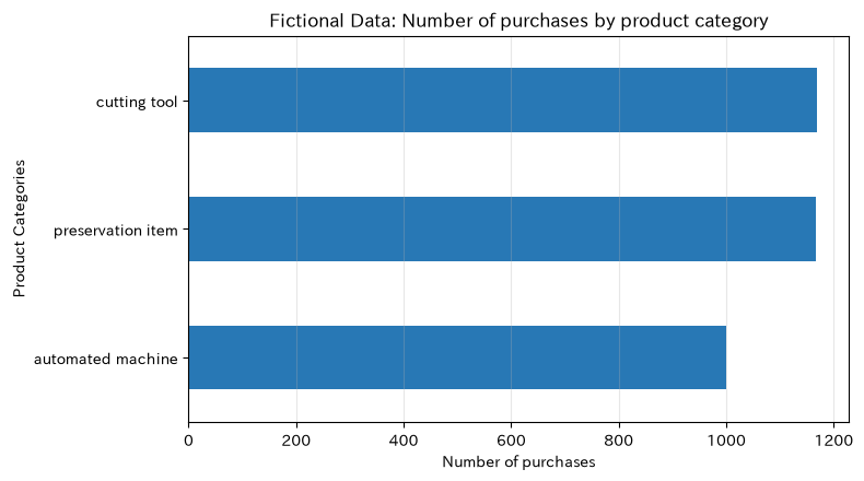

The data is sparse, and purchase volumes vary by category. This situation simplifies the difficulty of B2B recommendations, which prioritize unpurchased products based only on a small number of purchases. Below, we use the same data to compare the roles of each method.

7. No.061: Coordinated Filtering

Meaning in Practice

Customer base collaborative filtering is proposed to companies that have implemented similar purchases but have not yet purchased products from themselves. Even if the intended use is not specified, the strength lies in the ability to create horizontal deployment candidates based on purchasing patterns.

Approach to Analysis and Modeling

Using the purchase status vector as $\mathbf{x}_u$, and the cosine similarity of the customer $u,v$

$s(u,v)=\frac{\mathbf{x}_u^\top\mathbf{x}_v}{\lVert\mathbf{x}_u\rVert_2\lVert\mathbf{x}_v\rVert_2}$

Calculate it as follows. The score for Unpurchased Products $i$ is a value weighted by similarity by whether similar customers have purchased from them.

Check with Python

binary = (train > 0).astype(float)
norm = np.linalg.norm(binary, axis=1, keepdims=True)
similarity = binary @ binary.T / np.maximum(norm @ norm.T, 1e-12)
np.fill_diagonal(similarity, 0)
cf_scores = similarity @ binary / np.maximum(similarity.sum(axis=1, keepdims=True), 1e-12)
cf_scores[train > 0] = -np.inf

u = 72
top_cf = np.argsort(cf_scores[u])[-5:][::-1]
pd.DataFrame({"Recommended Products": np.array(item_ids)[top_cf], "CFScore": cf_scores[u, top_cf]}).merge(items, left_on="Recommended Products", right_on="item")

	Recommended Products	CFScore	item	category	gross_margin
0	P07	0.908	P07	preservation item	0.231
1	P13	0.876	P13	automated machine	0.231
2	P09	0.856	P09	preservation item	0.214
3	P08	0.828	P08	preservation item	0.332
4	P17	0.778	P17	automated machine	0.210

Reading the results

The score is not the purchase probability itself, but the strength of adoption at similar companies. Sales representatives can review equipment specifications and existing contracts for top candidates and propose cases along with case studies. On the other hand, for new customers or customers with few purchases, similarity is unstable, so supplementation with attribute information and popular products is necessary.

8. No.062：Matrix Factorization

Meaning in Practice

Matrix Factorization compresses a large table of customer×product products into a few latent axes. Latent axes can be interpreted as demand structures such as processing applications, maintenance focus, or automation investment, helping to generate candidates beyond explicit categories.

Approach to Analysis and Modeling

Approximate purchase matrix $R$ by the product of customer factor $P$ and product factor $Q$.

$R\approx PQ^\top,\qquad \min_{P,Q\geq0}\lVert R-PQ^\top\rVert_F^2$

Since the number of purchases is non-negative this time, we will use the easy-to-explain non-negative matrix factorization (NMF).

Check with Python

nmf = NMF(n_components=3, init="nndsvda", random_state=SEED, max_iter=1000)
P = nmf.fit_transform(train)
Q = nmf.components_.T
mf_scores = P @ Q.T
mf_scores[train > 0] = -np.inf

factor_profile = pd.DataFrame(Q, index=item_ids, columns=["latent axis1", "latent axis2", "latent axis3"])
for col in factor_profile:
    print(col, ":", ", ".join(factor_profile[col].nlargest(3).index))
top_mf = np.argsort(mf_scores[u])[-5:][::-1]
pd.DataFrame({"Recommended Products": np.array(item_ids)[top_mf], "MFScore": mf_scores[u, top_mf]})

Potential Axis 1: P13, P15, P18
Potential Axis 2: P05, P01, P09
Potential Axis 3: P12, P07, P09

	Recommended Products	MFScore
0	P13	0.365
1	P02	0.343
2	P09	0.312
3	P08	0.305
4	P07	0.299

Reading the results

When you line up products with significant weight along each latent axis, you can name the use cases represented by those axes using your business knowledge. However, factors are statistically obtained and do not necessarily have unique meanings. In sales meetings, the “factor name” is not definitively specified, but the common uses of higher-end products are confirmed as hypotheses.

9. No.063：Implicit Feedback

Meaning in Practice

There is no star rating in B2B order history. Actions such as purchase frequency, quote requests, and document viewing should be treated as Trust in the strength of interest rather than preferences.

Approach to Analysis and Modeling

We separate purchase $p_{ui}=\mathbb{1}[r_{ui}>0]$ and confidence $c_{ui}=1+\alpha\log(1+r_{ui})$ and consider weighted errors.

$\min_{P,Q}\sum_{u,i}c_{ui}(p_{ui}-\mathbf{p}_u^\top\mathbf{q}_i)^2+\lambda(\lVert P\rVert^2+\lVert Q\rVert^2)$

Here, you input a matrix multiplied by confidence into the NMF and confirm the concept in short code.

Check with Python

alpha = 3.0
confidence = 1 + alpha * np.log1p(train)
weighted_signal = (train > 0) * confidence
implicit_nmf = NMF(n_components=3, init="nndsvda", random_state=SEED, max_iter=1000)
Pu = implicit_nmf.fit_transform(weighted_signal)
Qi = implicit_nmf.components_.T
implicit_scores = Pu @ Qi.T
implicit_scores[train > 0] = -np.inf

sample = pd.DataFrame({"Number of purchases": np.arange(0, 11)})
sample["Reliability"] = 1 + alpha * np.log1p(sample["Number of purchases"])
sample

	Number of purchases	Reliability
0	0	1.000
1	1	3.079
2	2	4.296
3	3	5.159
4	4	5.828
5	5	6.375
6	6	6.838
7	7	7.238
8	8	7.592
9	9	7.908
10	10	8.194

Reading the results

Since the logarithm is used for the number of purchases, an increase from one to two is heavy, while an increase from ten to eleven is relatively milder. While preventing large corporations from monopolizing recommendations, repeat purchases can be used as strong evidence. In actual operations, different weights are assigned for viewing, quotation, and order receipt, and verification is conducted based on the negotiation rate.

10. No.064：LightGCN

Meaning in Practice

If you consider purchasing as the “edge connecting the customer node and the product node,” you can use a two- or third-step relationship of similar customers and similar products. LightGCN is a method that eliminates complex transformations and focuses on neighborhood propagation, which is crucial for recommendations.

Approach to Analysis and Modeling

Let the adjacency matrix of a two-part graph be $A$ and the degree matrix be $D$, then the normalized adjacency matrix is

$\tilde{A}=D^{-1/2}AD^{-1/2}$

That’s right. Embeddings are propagated as $E^{(k+1)}=\tilde{A}E^{(k)}$, and the average of each layer is the final representation. Here, we confirm two-layer propagation by embedding latent factors initially.

Check with Python

A = np.block([[np.zeros((n_customers, n_customers)), binary],
              [binary.T, np.zeros((n_items, n_items))]])
degree = A.sum(axis=1)
D_inv_sqrt = np.diag(1 / np.sqrt(np.maximum(degree, 1)))
A_norm = D_inv_sqrt @ A @ D_inv_sqrt
E0 = np.vstack([P, Q])
E1 = A_norm @ E0
E2 = A_norm @ E1
E = (E0 + E1 + E2) / 3
lightgcn_scores = E[:n_customers] @ E[n_customers:].T
lightgcn_scores[train > 0] = -np.inf

pd.DataFrame({
    "indicator": ["Number of nodes", "Number of edges", "matrix density"],
    "value": [A.shape[0], int(binary.sum()), round(A.mean(), 4)]
})

	indicator	value
0	Number of nodes	98.000
1	Number of edges	969.000
2	matrix density	0.202

Reading the results

The graph connects 80 customers and 18 products at the purchasing side. If propagation is made too deep, oversmoothing occurs where all nodes are represented similarly, so the number of layers is determined based on the validation data. In practice, data quality management, excluding discontinued products and technically incompatible areas, is also important.

11. No.065：Graph Neural Network

Meaning in Practice

GNN can integrate attributes such as customer industry, size, product category, and gross profit margin, not just purchasing relationships. It may help mitigate cold starts for new customers or new products with low purchase history.

Approach to Analysis and Modeling

Common message passing aggregates information from nearby $\mathcal{N}(v)$.

$\mathbf{h}_v^{(k+1)}=\sigma\left(W_{self}\mathbf{h}_v^{(k)}+W_{nei}\sum_{u\in\mathcal{N}(v)}\frac{\mathbf{h}_u^{(k)}}{\sqrt{d_ud_v}}\right)$

For full-scale learning, we use tools like PyTorch, but here, we further propagate the customer’s industry to the product side and visualize “which industries the product will be adopted.”

Check with Python

industry_onehot = pd.get_dummies(customers["industry"]).astype(float)
industry_signal = binary.T @ industry_onehot.to_numpy()
industry_share = industry_signal / np.maximum(industry_signal.sum(axis=1, keepdims=True), 1)
industry_df = pd.DataFrame(industry_share, index=item_ids, columns=industry_onehot.columns)

industry_df.plot(kind="bar", stacked=True, colormap="tab20c")
plt.title("GNNComposition by product type and recruitment industry equivalent to a first-stage consolidation")
plt.xlabel("Product Materials")
plt.ylabel("Industry Composition Ratio Among Acquiring Companies")
plt.grid(axis="y", alpha=0.3)
plt.legend(title="industry", bbox_to_anchor=(1.02, 1), loc="upper left")
plt.tight_layout()
plt.show()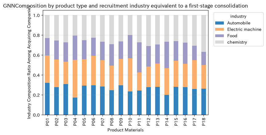

Reading the results

You can distinguish between products that are concentrated in specific industries and those that spread across multiple industries. For customers with fewer histories, products adopted in the same industry can be considered initial candidates. However, while industry attributes are convenient, there is a risk of entrenching past biases. Explicitly restrict the technical conditions that cannot be adopted, leaving room for exploration of new applications.

12. No.066: Diversity

Meaning in Practice

If all the top recommended tools are cutting tools, you will overlook the customer’s maintenance and automation needs. Diversity is an indicator that suppresses bias in proposal categories while maintaining accuracy.

Approach to Analysis and Modeling

Intra-list Diversity is calculated as the combination ratio of different categories.

$ILD(L)=\frac{2}{K(K-1)}\sum_{a<b}\mathbb{1}[category(i_a)\neq category(i_b)]$

For re-ranking, we use the MMR concept to adjust relevance and similarity to existing products.

Check with Python

cat_map = dict(zip(item_ids, item_category))
def diversity(indices):
    pairs = [(a, b) for x, a in enumerate(indices) for b in indices[x+1:]]
    return np.mean([item_category[a] != item_category[b] for a, b in pairs]) if pairs else 0

def diverse_rerank(scores, k=5, penalty=0.35):
    available, selected = set(np.flatnonzero(np.isfinite(scores))), []
    scaled = (scores - np.nanmin(scores[np.isfinite(scores)])) / (np.ptp(scores[np.isfinite(scores)]) + 1e-9)
    while available and len(selected) < k:
        best = max(available, key=lambda i: scaled[i] - penalty * sum(item_category[i] == item_category[j] for j in selected))
        selected.append(best); available.remove(best)
    return selected

base = np.argsort(mf_scores[u])[-5:][::-1].tolist()
reranked = diverse_rerank(mf_scores[u])
pd.DataFrame({
    "Method": ["Relevance only", "Diversity Re-ranking"],
    "Recommendation": [", ".join(np.array(item_ids)[base]), ", ".join(np.array(item_ids)[reranked])],
    "Diversity": [diversity(base), diversity(reranked)]
})

	Method	Recommendation	Diversity
0	Relevance only	P13, P02, P09, P08, P07	0.7
1	Diversity Re-ranking	P13, P02, P09, P08, P18	0.8

Reading the results

Re-ranking allows the category to expand beyond just the most relevant lists. If diversity becomes too high, unrelated proposals may be mixed in, so adjustments are made as weights for objective functions rather than constraints, and evaluations are made not only by click-through rate but also by the width of negotiations and multi-category order rates.

13. No.067: Serendipity

Meaning in Practice

Serendipity is a recommendation that is “surprising but useful for customers.” If you can present not just popular products but uses that the person in charge may have overlooked, it can lead to cross-selling and the deployment of new processes.

Approach to Analysis and Modeling

Usefulness is set as the model score, surprise as the unpopularity $-\log(pop_i)$, and simple indicators are

$Serendipity(u,i)=Relevance(u,i)\times[-\log(pop_i)]$

Let’s say so. Actual usefulness should be evaluated retrospectively through order acceptance and negotiations, and it is important not to overvalue products that are “just rare.”

Check with Python

popularity = binary.mean(axis=0)
finite = np.isfinite(mf_scores[u])
rel = np.zeros(n_items)
rel[finite] = (mf_scores[u, finite] - mf_scores[u, finite].min()) / (np.ptp(mf_scores[u, finite]) + 1e-9)
unexpectedness = -np.log(np.maximum(popularity, 1 / n_customers))
serendipity_score = rel * unexpectedness
serendipity_score[~finite] = -np.inf
top_ser = np.argsort(serendipity_score)[-5:][::-1]
pd.DataFrame({
    "Product Materials": np.array(item_ids)[top_ser],
    "Relevance": rel[top_ser],
    "Adoption rate": popularity[top_ser],
    "Serendipity": serendipity_score[top_ser]
})

	Product Materials	Relevance	Adoption rate	Serendipity
0	P02	0.935	0.588	0.498
1	P04	0.480	0.362	0.488
2	P18	0.735	0.575	0.406
3	P06	0.638	0.550	0.381
4	P14	0.374	0.375	0.367

Reading the results

Even if the adoption rate is low, highly relevant products rank high. These are considered separate ‘discovery frames’ from the usual proposal framework, and it is safer to present them with technical evidence and case studies. Since usefulness cannot be determined by offline metrics alone, record the reasons for sales reps’ acceptance or rejection and customer reactions.

14. No.068: Quantum Random Walk

Meaning in Practice

Random Walk moves along customer and product graphs to search for related candidates. In quantum random walks, it is possible to create search distributions different from classical methods by superimposing amplitudes and interference. However, in current practice, it is reasonable not to assume quantum dominance and to treat it as a comparative experiment.

Approach to Analysis and Modeling

A classic walk updates the probability vector to $\mathbf{p}_{t+1}=T\mathbf{p}_t$. The quantum discrete time walk is defined by the complex amplitude $|\psi_t\rangle$ as the unitary operator $U$

$|\psi_{t+1}\rangle=U|\psi_t\rangle,\qquad p_v=|\langle v|\psi_t\rangle|^2$

I will update you. Here, we do not implement quantum circuits but instead implement a classical random walk with restart as a comparison standard, clarifying the baseline at the time of research introduction.

Check with Python

transition = A / np.maximum(A.sum(axis=1, keepdims=True), 1)
start = np.zeros(A.shape[0]); start[u] = 1
p = start.copy(); restart = 0.2
for _ in range(30):
    p = (1 - restart) * transition.T @ p + restart * start
walk_scores = p[n_customers:].copy()
walk_scores[train[u] > 0] = -np.inf
top_walk = np.argsort(walk_scores)[-5:][::-1]
pd.DataFrame({"Product Materials": np.array(item_ids)[top_walk], "Probability of arrival": walk_scores[top_walk]})

	Product Materials	Probability of arrival
0	P07	0.021
1	P13	0.020
2	P09	0.020
3	P08	0.019
4	P17	0.018

Reading the results

The probability of reaching indicates the unpurchased products close to the customer on the graph. When considering quantum methods, it is important to measure improvements in accuracy, computation time, and implementation and operational costs relative to this classical baseline. Instead of deciding on production based solely on minor differences in the simulator, we prioritize a reproducible evaluation design.

15. No.069: Ranking Learning

Meaning in Practice

After generating candidates, not only recommendation scores but also gross profit, popularity, customer attributes, inventory, and proposal history are used to decide which one to show first. Ranking learning learns this order from past reactions.

Approach to Analysis and Modeling

In practice, there are pointwise, pairwise, and listwise methods. Here, each customer or product is treated as a single line, and the pointwise model is used, with purchase status as the objective variable, CF/MF score, popularity, and gross profit margin as explanatory variables. Use the HitRate@K to check ranking quality for evaluation.

$HitRate@K=\frac{1}{|U|}\sum_u\mathbb{1}[\text{The right productTop-Kincluded}]$

Check with Python

rows = []
raw_mf = P @ Q.T
for cu in range(70):
    for i in range(n_items):
        rows.append([cu, i, similarity[cu] @ binary[:, i], raw_mf[cu, i], popularity[i], items.loc[i, "gross_margin"], binary[cu, i]])
rank_df = pd.DataFrame(rows, columns=["u", "i", "cf", "mf", "pop", "margin", "label"])
X = rank_df[["cf", "mf", "pop", "margin"]]
y = rank_df["label"]
scaler = StandardScaler()
X_scaled = scaler.fit_transform(X)
ranker = LogisticRegression(class_weight="balanced", random_state=SEED, max_iter=1000).fit(X_scaled, y)

feature_table = pd.DataFrame({"Feature": X.columns, "coefficient": ranker.coef_[0]}).sort_values("coefficient", ascending=False)
feature_table

	Feature	coefficient
1	mf	1.926
0	cf	1.503
3	margin	-0.206
2	pop	-0.686

def hit_rate_at_k(score_matrix, pairs, k=5):
    hits = []
    for cu, true_i in pairs:
        top = np.argsort(score_matrix[cu])[-k:]
        hits.append(true_i in top)
    return np.mean(hits) if hits else np.nan

rank_scores = np.full((n_customers, n_items), -np.inf)
for cu in range(70, 80):
    feat = pd.DataFrame({
        "cf": similarity[cu] @ binary,
        "mf": raw_mf[cu],
        "pop": popularity,
        "margin": items["gross_margin"]
    })
    rank_scores[cu] = ranker.predict_proba(scaler.transform(feat))[:, 1]
    rank_scores[cu, train[cu] > 0] = -np.inf

comparison = pd.DataFrame({
    "Model": ["Collaborative filtering", "matrix factorization", "Ranking Learning"],
    "HitRate@5": [hit_rate_at_k(cf_scores, test_pairs), hit_rate_at_k(mf_scores, test_pairs), hit_rate_at_k(rank_scores, test_pairs)]
})
comparison

	Model	HitRate@5
0	Collaborative filtering	1.0
1	matrix factorization	0.8
2	Ranking Learning	0.9

Reading the results

Since the coefficients are standardized after standardization, you can compare which features contributed to the ranking by direction and size. HitRate for small-scale hypothetical data does not generalize the superiority of a method. In practice, the learning and evaluation periods are divided over time, with HitRate, NDCG, negotiation rate, and expected gross margin listed together, and only profit is monitored to ensure customer fit is not compromised.

16. No.070: Online Learning

Meaning in Practice

Customer interests change with equipment upgrades, budget deadlines, and new product launches. Online learning receives new responses such as browsing and inquiries, and updates recommendation policies continuously. By leaving exploration, we provide learning opportunities even for products with little track record.

Approach to Analysis and Modeling

In UCB (Upper Confidence Bound), a multi-skilled bandit, the average reward for product $i$ is $\hat\mu_i$ and the number of trials is $n_i$.

$UCB_i(t)=\hat\mu_i+c\sqrt{\frac{\log t}{n_i}}$

We present products that maximize these benefits. Section 1 is about utilization, and section 2 is exploration. Here, with the customer response rate set to be unknown, we simulate 500 proposals.

Check with Python

true_response = np.array([0.06, 0.10, 0.04, 0.16, 0.08])
n_arms, rounds, c = len(true_response), 500, 1.2
trials = np.zeros(n_arms); rewards = np.zeros(n_arms)
cumulative = []
for t in range(1, rounds + 1):
    if t <= n_arms:
        arm = t - 1
    else:
        mean = rewards / trials
        ucb = mean + c * np.sqrt(np.log(t) / trials)
        arm = np.argmax(ucb)
    reward = rng.random() < true_response[arm]
    trials[arm] += 1; rewards[arm] += reward
    cumulative.append(rewards.sum())

pd.DataFrame({
    "Candidate": [f"Candidate{i+1}" for i in range(n_arms)],
    "True response rate (for verification)": true_response,
    "Reminder count": trials.astype(int),
    "estimated reaction rate": rewards / trials
})

	Candidate	True response rate (for verification)	Reminder count	estimated reaction rate
0	Candidate1	0.06	78	0.064
1	Candidate2	0.10	113	0.124
2	Candidate3	0.04	78	0.064
3	Candidate4	0.16	171	0.175
4	Candidate5	0.08	60	0.017

plt.plot(np.arange(1, rounds + 1), cumulative, color="#D95319")
plt.title("UCBCumulative number of responses to online proposals")
plt.xlabel("Number of Proposals")
plt.ylabel("Cumulative number of responses")
plt.grid(alpha=0.3)
plt.tight_layout()
plt.show()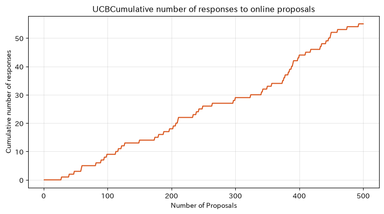

Reading the results

While candidates with high response rates are being offered, other candidates are also being explored. Since feedback is slow when only orders are received during the actual event, intermediary compensation is designed to include document review, inquiries, and business negotiations. Exploration should be limited to areas that do not compromise the customer experience, and guardrails must be implemented to exclude discontinued or non-compliant items from the list of candidates.

17. Practical Insights Seen Through Target Exercise

The 10 methods are not competing single models, but rather components of the recommended work.

layer	Main Methods	Decision-making
candidate generation	CF, MF, Implicit, LightGCN/GNN, Random Walk	Reducing missed proposals
Re-ranking	Diversity, Serendipity, and Ranking Learning	Decide the order and the breadth of the proposal
Learning and Operation	Online Learning	Keeping up with changes in response

The most important aspect is not high offline accuracy, but a series of business designs that allow sales to verify the reasons for recommendations, exclude suggestions that are disadvantageous to the customer, and return the results to the next learning session.

18. What is necessary for practical implementation

1. Agreement on purpose: Decide which main objectives are sales, gross profit, negotiation rate, or reactivating dormant customers.
2. IDand data organization: Integrate customer, location, and product codes to identify returns, discontinued items, and free samples
3. fitness constraint: Set equipment specifications, certifications, regions, inventory, and contract terms as rules before and after recommendations
4. Time-series evaluation: Learn from the past and predict the future, comparing popular models and current sales operations
5. Explanation and Screen Design: Display recommendation reasons such as “Adopted by similar companies” or “Often used in combination with existing products”
6. feedback loop: Record reasons for hiring or holding off, customer reactions, and orders
7. Monitoring and Control: Continuously monitor accuracy, bias, search rates, data drift, and sales ban conditions

19. Summary

Starting from purchase history, No.061 to 070 expanded the recommendation system to include latent factors, implicit feedback, graph structure, attributes, diversity, surprise, rankings, and sequential learning.

Recommendations for manufacturing companies are not enough just to “release products that seem likely to be successful.” By creating verifiable proposal hypotheses for sales while maintaining technical suitability, and returning customer responses back to learning, it becomes a foundation for continuous decision-making. It is realistic to start with small-scale tests targeting targeted customers and products, then compare them with current sales to confirm effectiveness.

20. Consultations for Corporations

At Surikoubo, we support the conceptualization and organization of recommendation systems using manufacturing orders, customers, and product data, as well as PoC, evaluation design, and business implementation. You can consult from stages such as “We have data but can’t use it for proposals” or “We want to connect model accuracy with sales operations.”

📩 Contact Us: surikobo.co.jp/contact Please feel free to consult us first.