10 Practices to Optimize Sales and Marketing Investment in Manufacturing

No.081–No.090: From Policy Contribution to Digital Twins and Decision Intelligence

Assuming industrial equipment manufacturers, we evaluate multiple measures including exhibitions, technical seminars, web advertising, and agency support, including Order Probability, Gross Profit, Supply Constraints, Uncertainty. Instead of listing individual analytical methods, treat them as a practical workflow: “measuring the contribution of measures→ creating allocation plans→ confirming tolerance for fluctuations, → making decisions in meetings.”

[!NOTE] This material is a notebook previously used by Surikoubo (or personally by the representative, Kazuyama), and has been reconstructed, edited, and published with the company’s permission.
All data listed is fictional and has no relation whatsoever to real companies, factories, or figures.

Introduction: Practical Challenges in Manufacturing Covered in This Article

In B2B manufacturing, it takes several months from investing marketing expenses to receiving orders, with customers passing through multiple touchpoints. Furthermore, sales staff, factory capacity, product-specific gross profit, and material shortages all affect results. The question in this article is not simply “maximizing leads,” but Where to allocate the limited budget, what uncertainty to tolerate, and who makes decisions under what conditions.

Common situations on site

• Exhibitions are close to orders but expensive, while web ads have many touchpoints but are far from orders.
• Each department evaluates initiatives based on its own KPIs, and the connection with company-wide gross profit is weak.
• Average-based plans collapse due to demand fluctuations and supply constraints.
• Even if you create an advanced model, you can’t explain its adoption in meetings and it won’t be put into practice.

Why is this issue so difficult to judge?

This is because the order of customer touchpoints, overlap between measures, diminishing effects, intteger budget values, future demand distribution, and model errors all exist simultaneously. If you allocate based solely on correlation, you may be overvalued, and if you optimize based solely on expected values, you will miss significantly under poor conditions. Therefore, in this article, we compare multiple perspectives and clearly state the objective function and constraints.

Overview of Exercise covered this time

No.	Theme	Role in Decision-Making
081	Attribution	Distribute contributions from the points of contact leading to orders
082	Portfolio optimization	Balancing revenue and volatility
083	Simulation optimization	Exploring complex tasks through iterative computation
084	Robust optimization	Choose a solution that’s hard to break even under worst-case conditions
085	Probability optimization	Managing the probability of constraint violations
086	Reinforcement Learning	Allocate sequentially based on observation results
087	Digital twin	Virtually recreating everything from initiatives to production
088	Integration with DI	Connecting Analytics to the Decision-Making Process
089	Optimization in the AI Era	Using AI predictions for monitorable optimization
090	Practical Examples	Seamlessly Handle Implementation Decisions

Preparing the Python environment

It does not rely on external data and uses only NumPy, pandas, and matplotlib. Fix the random number seed so you can reproduce the same result. Unless otherwise noted, the unit of amount is 10,000 yen.

%matplotlib inline
import sys
import numpy as np
import pandas as pd
import matplotlib
import matplotlib.pyplot as plt
from itertools import product

SEED = 42
rng = np.random.default_rng(SEED)
pd.set_option("display.float_format", lambda x: f"{x:,.2f}")
print("Python:", sys.version.split()[0])
print("numpy:", np.__version__, "pandas:", pd.__version__, "matplotlib:", matplotlib.__version__)

Python: 3.13.1
numpy: 2.5.1 pandas: 3.0.3 matplotlib: 3.11.0

Creation of Fictional Data

We will have the most recent 400 business negotiations for the industrial pump manufacturer ‘Kobo Pump.’ Each negotiation involves multiple customer touchpoints, including project scale, product, order results, and gross margin. The true order probability is only available at the time of data generation and cannot be observed in practice.

channels = ["Exhibition", "WebAds", "Webinar", "Distributor"]
products = ["Standard", "HighPressure", "IoT"]
n = 400
deal_size = rng.lognormal(mean=4.5, sigma=0.45, size=n)
product_category = rng.choice(products, size=n, p=[0.45, 0.30, 0.25])
touches = rng.poisson([0.7, 1.4, 0.9, 0.8], size=(n, 4))
touches = np.clip(touches, 0, 4)
linear = -2.7 + touches @ np.array([0.55, 0.18, 0.40, 0.48]) + 0.20 * (product_category == "IoT")
win_prob = 1 / (1 + np.exp(-linear))
won = rng.binomial(1, win_prob)
margin_rate = np.select([product_category == "Standard", product_category == "HighPressure"], [0.28, 0.34], default=0.42)
deals = pd.DataFrame(touches, columns=channels)
deals.insert(0, "deal_id", [f"D{i:04d}" for i in range(1, n + 1)])
deals["product"] = product_category
deals["deal_size"] = deal_size
deals["won"] = won
deals["gross_profit"] = deal_size * margin_rate * won
print("Number of Fictional Data Entries:", len(deals), " / Order rate:", f"{deals.won.mean():.1%}")
deals.head()

Number of fictitious data items: 400 / Order rate: 22.0%

	deal_id	Exhibition	WebAds	Webinar	Distributor	product	deal_size	won	gross_profit
0	D0001	1	1	0	1	Standard	103.25	0	0.00
1	D0002	2	1	1	1	IoT	56.37	0	0.00
2	D0003	0	3	2	0	Standard	126.18	0	0.00
3	D0004	1	1	1	1	IoT	137.45	0	0.00
4	D0005	1	0	2	1	HighPressure	37.41	0	0.00

No.081: Attribution

Meaning in Practice

If orders are attributed only to the final touchpoint, upstream measures effective in project development are underestimated. On the other hand, distributing evenly across all touchpoints ignores the order and order relationships. Here, we compare the gross profit from received projects using two methods: ‘final contact’ and ‘proportional allocation of contact counts’ to confirm that evaluation rules change budget decisions.

Approach to Analysis and Modeling

If the gross profit of deal $i$ is $G_i$ and the number of contacts in channel $j$ is $x_{ij}$, then the linear allocation amount is

$A_j=\sum_i G_i\frac{x_{ij}}{\sum_k x_{ik}}$

That’s right. This is not a causal effect but a Accounting Allocation to the observed contact points. Causality requires separate experiments and control groups.

Check with Python

won_deals = deals.query("won == 1").copy()
denom = won_deals[channels].sum(axis=1).replace(0, np.nan)
linear_credit = won_deals[channels].div(denom, axis=0).mul(won_deals["gross_profit"], axis=0).sum().fillna(0)
last_touch = won_deals[channels].apply(lambda r: channels[np.flatnonzero(r.to_numpy() > 0)[-1]] if r.sum() else "None", axis=1)
last_credit = won_deals.groupby(last_touch)["gross_profit"].sum().reindex(channels, fill_value=0)
attr = pd.DataFrame({"Linear credit": linear_credit, "Last-touch credit": last_credit})
display(attr.round(1))
ax = attr.plot(kind="bar", figsize=(8, 4), color=["#2F6690", "#D95F59"])
ax.set(title="Gross-profit attribution by rule", xlabel="Channel", ylabel="Attributed gross profit (10k JPY)")
ax.grid(axis="y", alpha=.3); plt.xticks(rotation=0); plt.tight_layout(); plt.show()

	Linear credit	Last-touch credit
Exhibition	590.80	33.80
WebAds	944.50	392.40
Webinar	666.80	681.70
Distributor	566.00	1,660.30

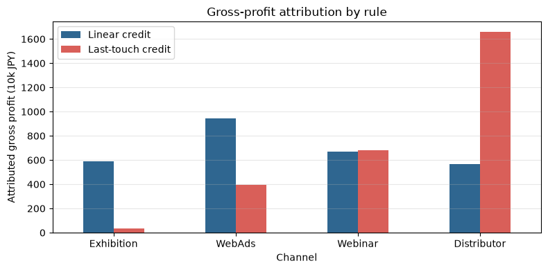
Reading the results

The channel’s ranking and amount will change depending on the distribution method. Therefore, the “contribution amount” is not a fact but an indicator that includes rules. In practice, allocation indicators are not the sole basis for budget cuts; instead, the order of contact points, project attributes, and untouched control groups are listed together.

No.082: Portfolio Optimization

Meaning in Practice

Even if the average ROI by policy is high, focusing on initiatives that simultaneously deteriorate under the same economic factors can cause plans to become unstable. Applying the investment portfolio concept, we simultaneously look at expected gross profit and variable risk.

Approach to Analysis and Modeling

If the allocation ratio is $w$, expected return is $\mu$, and covariance matrix is $\Sigma$, the expected return is $w^T\mu$ and the risk is $\sqrt{w^T\Sigma w}$. Here, we explore all allocation options in 5% increments to maximize risk-adjusted score $w^T\mu-\lambda\sqrt{w^T\Sigma w}$.

Check with Python

scenario_returns = pd.DataFrame({
    "Exhibition": [0.55, 0.30, 0.12, 0.40, 0.20, 0.48],
    "WebAds": [0.38, 0.42, 0.18, 0.35, 0.28, 0.31],
    "Webinar": [0.44, 0.36, 0.25, 0.40, 0.32, 0.39],
    "Distributor": [0.32, 0.24, 0.40, 0.29, 0.45, 0.35],
}, index=["Boom", "Normal-A", "Recession", "Normal-B", "SupplyShock", "Recovery"])
mu, cov = scenario_returns.mean().to_numpy(), scenario_returns.cov().to_numpy()
candidates = []
for units in product(range(21), repeat=4):
    if sum(units) == 20:
        w = np.array(units) / 20
        ret, risk = w @ mu, np.sqrt(w @ cov @ w)
        candidates.append([*w, ret, risk, ret - 1.2 * risk])
portfolio = pd.DataFrame(candidates, columns=channels + ["expected_return", "risk", "score"])
best_port = portfolio.loc[portfolio.score.idxmax()]
display(best_port.to_frame("value").round(3))
plt.figure(figsize=(7, 4)); plt.scatter(portfolio.risk, portfolio.expected_return, s=10, alpha=.35)
plt.scatter(best_port.risk, best_port.expected_return, s=90, color="#D95F59", label="Selected")
plt.title("Marketing portfolio: return and risk"); plt.xlabel("Risk (standard deviation)"); plt.ylabel("Expected return")
plt.grid(alpha=.3); plt.legend(); plt.tight_layout(); plt.show()

	value
Exhibition	0.00
WebAds	0.00
Webinar	0.55
Distributor	0.45
expected_return	0.35
risk	0.03
score	0.31

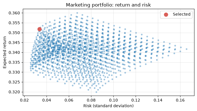
Reading the results

The options are not just about maximizing average returns, but about combining them to minimize fluctuations between business scenarios. Since the risk factor $\lambda$ represents the management tolerance, analysts do not implicitly decide this but compare multiple proposals at management meetings.

No.083: Simulation Optimization

Meaning in Practice

Exhibition visitors, business negotiations, and orders are probabilistic. Even if it is difficult to create closed formulas, you can virtually run candidate budgets multiple times to compare gross profit distributions.

Approach to Analysis and Modeling

For each initiative’s investment unit $b_j$, the number of deals is generated using a Poisson distribution and the number of orders received is generated using a binomial distribution. The goal is to maximize expected net gross profit $E[G(b)-C(b)]$. However, to avoid overlearning, record candidate counts, iterations, and random number management.

Check with Python

def simulate_plan(units, repeats=800, seed=SEED):
    local = np.random.default_rng(seed)
    units = np.asarray(units)
    leads_per_unit = np.array([7, 12, 9, 8])
    win_rate = np.array([.24, .11, .19, .22])
    gp_per_win = np.array([70, 48, 62, 58])
    cost_per_unit = np.array([80, 35, 45, 50])
    leads = local.poisson(units * leads_per_unit, size=(repeats, 4))
    wins = local.binomial(leads, win_rate)
    return (wins * gp_per_win).sum(axis=1) - units @ cost_per_unit

plans = []
for u in product(range(5), repeat=4):
    if np.dot(u, [80, 35, 45, 50]) <= 400:
        profit = simulate_plan(u)
        plans.append([u, profit.mean(), np.quantile(profit, .10)])
sim_result = pd.DataFrame(plans, columns=["units", "mean_profit", "p10_profit"]).sort_values("mean_profit", ascending=False)
display(sim_result.head(8))
top = sim_result.head(3)
plt.figure(figsize=(8, 4))
for _, row in top.iterrows():
    plt.hist(simulate_plan(row.units), bins=25, alpha=.35, label=str(row.units))
plt.title("Profit distribution of top simulated plans"); plt.xlabel("Net gross profit (10k JPY)"); plt.ylabel("Frequency")
plt.grid(alpha=.3); plt.legend(title="Units"); plt.tight_layout(); plt.show()

	units	mean_profit	p10_profit
71	(0, 2, 4, 3)	457.61	157.20
24	(0, 0, 4, 4)	436.67	158.00
93	(0, 3, 4, 2)	433.58	146.60
48	(0, 1, 4, 3)	431.04	168.80
90	(0, 3, 3, 3)	424.48	148.00
44	(0, 1, 3, 4)	422.85	155.80
155	(1, 1, 4, 2)	413.90	143.00
86	(0, 3, 2, 4)	410.49	133.00

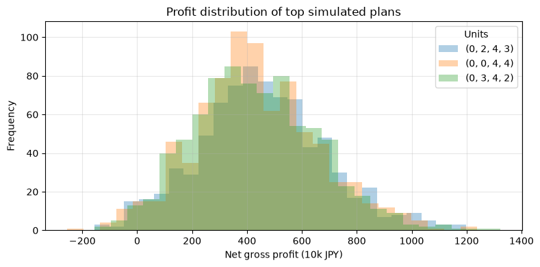
Reading the results

Even proposals with similar expectations can have differences in the bottom 10%. If management dislikes budget reductions, there is room to choose a plan with a higher P10 rather than the maximum average. Also, increase the number of iterations and double-check to ensure that random error does not affect ranking.

No.084: Robust Optimization

Meaning in Practice

Estimates of order rates may not remain the same in the future. Robust optimization places the “most unfavorable scenario within the expected range” and selects solutions that can ensure results even in those situations.

Approach to Analysis and Modeling

For an uncertain set of scenarios $S$, solve $\max_b\min_{s\in S}G(b,s)$. If you become overly pessimistic, you may stop investing, so the uncertainty set is set to be explainable based on past fluctuations and expert judgment.

Check with Python

base = np.array([.24, .11, .19, .22])
shocks = pd.DataFrame([
    base,
    base * [.70, .90, .85, 1.00],
    base * [.95, .65, .80, .95],
    base * [.80, .85, .70, .90],
], index=["Base", "EventWeak", "DigitalWeak", "BroadDownturn"], columns=channels)
robust_rows = []
for u in product(range(5), repeat=4):
    cost = np.dot(u, [80, 35, 45, 50])
    if cost <= 400:
        scenario_profit = (np.asarray(u) * np.array([7,12,9,8]) * shocks.to_numpy() * np.array([70,48,62,58])).sum(axis=1) - cost
        robust_rows.append([u, scenario_profit.mean(), scenario_profit.min()])
robust = pd.DataFrame(robust_rows, columns=["units", "average", "worst_case"])
best_robust = robust.loc[robust.worst_case.idxmax()]
display(best_robust.to_frame("robust plan").round(1))
comparison = pd.DataFrame({"Mean-optimal": sim_result.iloc[0][["mean_profit", "p10_profit"]],
                           "Robust": [best_robust.average, best_robust.worst_case]}, index=["Average-like", "Downside metric"])
comparison.plot(kind="bar", figsize=(7,4), color=["#2F6690", "#E6A23C"])
plt.title("Mean-oriented and robust plans"); plt.xlabel("Metric"); plt.ylabel("Net gross profit (10k JPY)")
plt.grid(axis="y", alpha=.3); plt.xticks(rotation=0); plt.tight_layout(); plt.show()

	robust plan
units	(0, 0, 4, 4)
average	368.18
worst_case	284.34

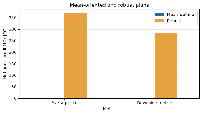
Reading the results

The robust plan partially gives up average growth to limit losses in weak scenarios. You don’t always have to use the entire budget, and if marginal profit is uncertain, leaving some investment room can be the best solution.

No.085: Probability Optimization

Meaning in Practice

If the factory cannot process the orders won by sales, delivery delays and missed opportunities occur. Rather than “within the average capability,” the probability of exceeding the capability must be kept below a certain level.

Approach to Analysis and Modeling

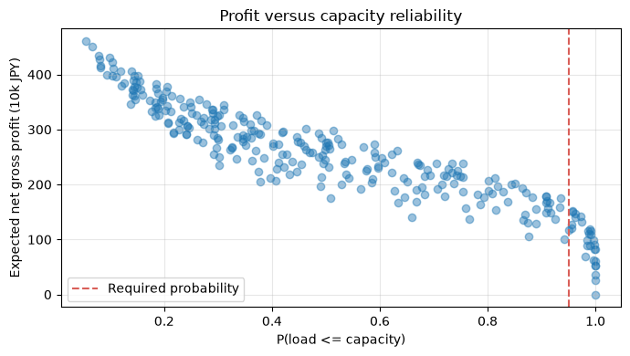
Let production load be $L(b,\xi)$ random variables, monthly capacity $C$, and an opportunity constraint $P(L\le C)\ge 1-\alpha$. Here, we estimate the fulfillment rate using the Monte Carlo sample, adopting only proposals with 95% or higher potential.

Check with Python

def capacity_check(units, repeats=2000, seed=123):
    local = np.random.default_rng(seed)
    units = np.asarray(units)
    leads = local.poisson(units * [7,12,9,8], size=(repeats,4))
    wins = local.binomial(leads, [.24,.11,.19,.22])
    load = wins @ np.array([18, 12, 16, 15])
    profit = wins @ np.array([70,48,62,58]) - units @ np.array([80,35,45,50])
    return profit.mean(), (load <= 135).mean(), np.quantile(load, .95)

chance_rows = []
for u in product(range(5), repeat=4):
    if np.dot(u, [80,35,45,50]) <= 400:
        mean_profit, service_prob, load_p95 = capacity_check(u)
        chance_rows.append([u, mean_profit, service_prob, load_p95])
chance = pd.DataFrame(chance_rows, columns=["units", "mean_profit", "capacity_probability", "load_p95"])
feasible = chance.query("capacity_probability >= 0.95").sort_values("mean_profit", ascending=False)
display(feasible.head(8))
plt.figure(figsize=(7,4)); plt.scatter(chance.capacity_probability, chance.mean_profit, alpha=.45)
plt.axvline(.95, color="#D95F59", linestyle="--", label="Required probability")
plt.title("Profit versus capacity reliability"); plt.xlabel("P(load <= capacity)"); plt.ylabel("Expected net gross profit (10k JPY)")
plt.grid(alpha=.3); plt.legend(); plt.tight_layout(); plt.show()

	units	mean_profit	capacity_probability	load_p95
35	(0, 1, 2, 0)	151.88	0.96	132.00
3	(0, 0, 0, 3)	149.74	0.96	135.00
77	(0, 3, 1, 0)	146.38	0.96	128.00
31	(0, 1, 1, 1)	141.55	0.97	127.05
73	(0, 3, 0, 1)	139.68	0.96	129.00
27	(0, 1, 0, 2)	132.30	0.97	126.00
140	(1, 1, 1, 0)	126.77	0.96	134.00
136	(1, 1, 0, 1)	119.75	0.96	132.00

Reading the results

Only the dot on the right meets 95% of the capability constraints. The 5% probability of exceeding the allowable limit is not a technical constant, but a management decision based on overtime, outsourcing, delivery contracts, and customer importance.

No.086: Reinforcement Learning

Meaning in Practice

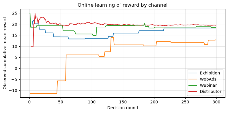
In new markets where the effectiveness of these measures is unclear, it is more reasonable to update allocations while learning with small amounts rather than fixing the annual budget based solely on initial estimates. Here, we will treat multi-armed bandits as the entry point for reinforcement learning.

Approach to Analysis and Modeling

In the $\varepsilon$-greedy method, the strategy with the highest estimated value is selected by probability $1-\varepsilon$ and explored by probability $\varepsilon$. The value is updated sequentially at $Q_{t+1}(a)=Q_t(a)+(R_t-Q_t(a))/N_t(a)$.

Check with Python

true_value = np.array([18, 12, 16, 20])
bandit_rng = np.random.default_rng(SEED)
q = np.zeros(4); counts = np.zeros(4, dtype=int); history = []
epsilon = .15
for t in range(300):
    if bandit_rng.random() < epsilon or counts.min() == 0:
        a = bandit_rng.integers(4)
    else:
        a = int(np.argmax(q))
    reward = bandit_rng.normal(true_value[a], 12)
    counts[a] += 1
    q[a] += (reward - q[a]) / counts[a]
    history.append((t, a, reward, q[a]))
bandit = pd.DataFrame({"channel": channels, "trials": counts, "estimated_value": q, "true_value_demo_only": true_value})
display(bandit.round(2))
plt.figure(figsize=(8,4))
for j, ch in enumerate(channels):
    series = pd.Series([h[2] if h[1] == j else np.nan for h in history]).expanding().mean()
    plt.plot(series, label=ch)
plt.title("Online learning of reward by channel"); plt.xlabel("Decision round"); plt.ylabel("Observed cumulative mean reward")
plt.grid(alpha=.3); plt.legend(); plt.tight_layout(); plt.show()

	channel	trials	estimated_value	true_value_demo_only
0	Exhibition	14	18.23	18
1	WebAds	14	12.91	12
2	Webinar	17	18.49	16
3	Distributor	255	19.52	20

Reading the results

While efforts are gathering on measures with observed high rewards, exploration continues. In practice, pay attention to delayed rewards being observed, differences in customer attributes, and changes in policies that can harm the customer experience, and establish guardrails and manual stoppage authority.

No.087: Digital Twin

Meaning in Practice

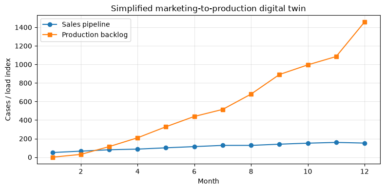
Marketing decisions ripple through sales and production. The digital twin is a system that recreates the transitions from policy implementation to business negotiations, order receipts, production loads, and delivery dates in a virtual space, confirming cross-departmental impacts.

Approach to Analysis and Modeling

Here, we create a simple monthly state model. The status is $P_t$ project and production $B_t$, and the input is measure volume $u_t$. $P_{t+1}=P_t+Leads(u_t)-Wins_t$ updates $B_{t+1}=\max(0,B_t+Load(Wins_t)-Capacity)$.

Check with Python

def run_twin(monthly_units, months=12, seed=77):
    local = np.random.default_rng(seed); pipeline = 20; backlog = 10; rows = []
    for month in range(1, months+1):
        leads = local.poisson(np.dot(monthly_units, [7,12,9,8]))
        available = pipeline + leads
        wins = local.binomial(available, .12)
        pipeline = available - wins
        new_load = wins * local.integers(12, 20)
        capacity = 135 + local.integers(-10, 11)
        backlog = max(0, backlog + new_load - capacity)
        rows.append([month, leads, wins, pipeline, new_load, capacity, backlog])
    return pd.DataFrame(rows, columns=["month","leads","wins","pipeline","new_load","capacity","backlog"])

twin = run_twin(feasible.iloc[0].units)
display(twin)
fig, ax = plt.subplots(figsize=(8,4))
ax.plot(twin.month, twin.pipeline, marker="o", label="Sales pipeline")
ax.plot(twin.month, twin.backlog, marker="s", label="Production backlog")
ax.set(title="Simplified marketing-to-production digital twin", xlabel="Month", ylabel="Cases / load index")
ax.grid(alpha=.3); ax.legend(); plt.tight_layout(); plt.show()

	month	leads	wins	pipeline	new_load	capacity	backlog
0	1	35	5	50	90	132	0
1	2	27	12	65	156	126	30
2	3	28	13	80	221	137	114
3	4	23	16	87	240	145	209
4	5	33	19	101	247	128	328
5	6	27	14	114	238	127	439
6	7	24	11	127	209	133	515
7	8	21	21	127	294	129	680
8	9	36	23	140	345	134	891
9	10	25	14	151	238	134	995
10	11	24	16	159	224	134	1085
11	12	20	27	152	513	141	1457

Reading the results

Even if negotiations increase, if there are months when unfinished production accumulates, delivery risk rises. During implementation, it is necessary to align definitions and update times for CRM, order processing, and MES/ERP, and continuously monitor discrepancies with reality. It’s not just precise 3D models that are digital twins.

No.088: Integration with DI

Meaning in Practice

DI (Decision Intelligence) is a concept that integrates the results of forecasting and optimization into business processes, including decision-makers, options, rationale, approvals, and performance verification. We design not only model accuracy but also “who looks at what, and when to decide.”

Approach to Analysis and Modeling

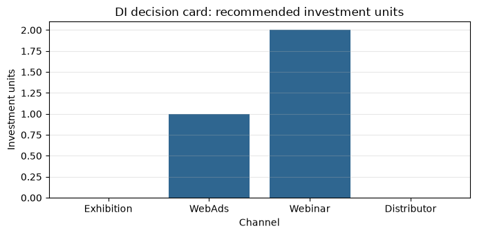
In DI, objectives, constraints, choices, recommendations, reliability, and guardrails are recorded as decision records. This allows you to track where to improve the model, inputs, constraints, and approval decisions when results are poor.

Check with Python

selected = feasible.iloc[0]
decision_record = pd.DataFrame([
    ["Objective", "Expected net gross profit", f"{selected.mean_profit:.1f}"],
    ["Decision", "Investment units", dict(zip(channels, selected.units))],
    ["Constraint", "Budget", "<= 400 (10k JPY)"],
    ["Guardrail", "P(production load <= capacity)", f"{selected.capacity_probability:.1%}"],
    ["Owner", "Approval", "Sales, Marketing, Production, Finance"],
    ["Review", "Re-estimation", "Monthly / stop if reliability < 90%"],
], columns=["record_type", "item", "value"])
display(decision_record)
plt.figure(figsize=(7,3.5)); plt.bar(channels, selected.units, color="#2F6690")
plt.title("DI decision card: recommended investment units"); plt.xlabel("Channel"); plt.ylabel("Investment units")
plt.grid(axis="y", alpha=.3); plt.tight_layout(); plt.show()

	record_type	item	value
0	Objective	Expected net gross profit	151.9
1	Decision	Investment units	{'Exhibition': 0, 'WebAds': 1, 'Webinar': 2, '...
2	Constraint	Budget	<= 400 (10k JPY)
3	Guardrail	P(production load <= capacity)	95.8%
4	Owner	Approval	Sales, Marketing, Production, Finance
5	Review	Re-estimation	Monthly / stop if reliability < 90%

Reading the results

Not only recommended values, but also constraints, reliability, accountability, and re-evaluation conditions all form a single record. This is the smallest unit to move from “analytical data” to “actionable decision-making.” DI is not a specific product name, but rather a framework for designing, recording, and improving decision-making.

No.089: Optimization in the AI Era

Meaning in Practice

Generative AI and predictive AI can assist with project summarization, contract probabilities, and strategy proposals. However, if AI’s predictions are passed directly to optimization, overconfidence and distribution changes can distort the distribution.

Approach to Analysis and Modeling

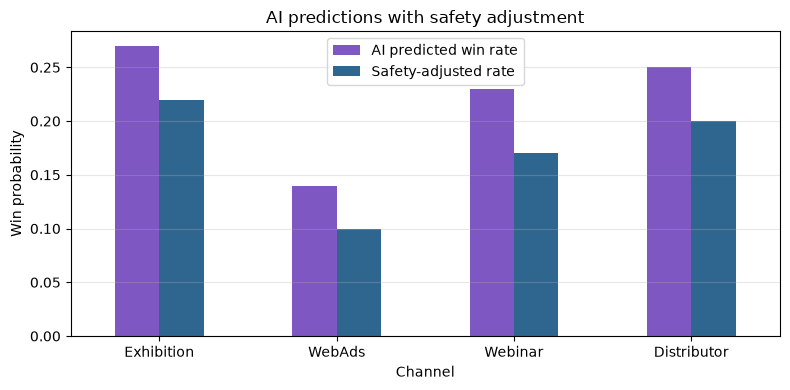
If AI prediction is set to $\hat p$, it corrects for the safety side $p_{safe}=\mathrm{clip}(\hat p-m,0,1)$ based on calibration errors and drift, and inputs it into constrained optimization. Additionally, the reason for recommendation, input version, approver, and achievements are recorded in the audit log.

Check with Python

ai_pred = pd.Series([.27, .14, .23, .25], index=channels, name="AI predicted win rate")
uncertainty_margin = pd.Series([.05, .04, .06, .05], index=channels)
safe_pred = (ai_pred - uncertainty_margin).clip(0, 1).rename("Safety-adjusted rate")
ai_table = pd.concat([ai_pred, uncertainty_margin.rename("Uncertainty margin"), safe_pred], axis=1)
display(ai_table)
ax = ai_table[["AI predicted win rate", "Safety-adjusted rate"]].plot(kind="bar", figsize=(8,4), color=["#7E57C2", "#2F6690"])
ax.set(title="AI predictions with safety adjustment", xlabel="Channel", ylabel="Win probability")
ax.grid(axis="y", alpha=.3); plt.xticks(rotation=0); plt.tight_layout(); plt.show()

	AI predicted win rate	Uncertainty margin	Safety-adjusted rate
Exhibition	0.27	0.05	0.22
WebAds	0.14	0.04	0.10
Webinar	0.23	0.06	0.17
Distributor	0.25	0.05	0.20

Reading the results

Safety-side forecasts with margins of uncertainty are more modest than AI’s point predictions. The key is not to blindly doubt AI, but to measure calibration errors, out-of-target data, and input defects, and adjust automation levels according to confidence levels.

No.090: Practical Case Study—Recreating Quarterly Investment Meetings

Meaning in Practice

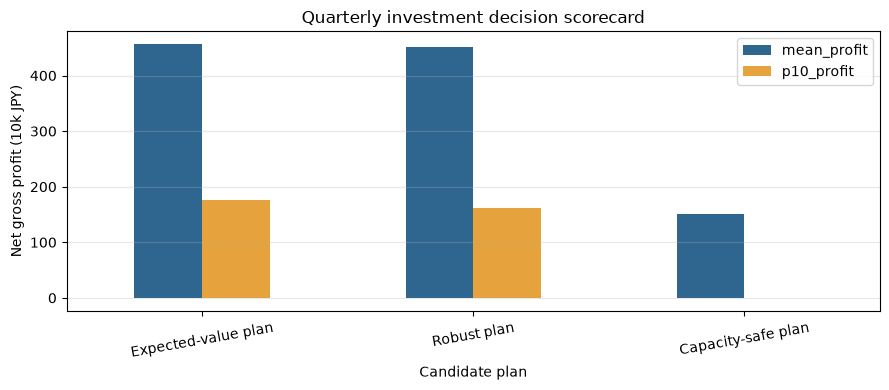
Finally, compare the candidates as a hypothetical quarterly investment meeting. Average gross profit, downward turn, capacity fulfillment ratio, and budget are all presented in the same table, and consensus is formed based on multiple criteria rather than a single KPI.

Approach to Analysis and Modeling

The candidates are three options: “Emphasis on Expected Value,” “Robust,” and “With Ability Constraints.” In decision-making, Pareto superiority, hard constraints, and acceptable risk are reviewed in that order. Models visualize trade-offs rather than replace decision-making.

Check with Python

candidate_units = {
    "Expected-value plan": tuple(sim_result.iloc[0].units),
    "Robust plan": tuple(best_robust.units),
    "Capacity-safe plan": tuple(feasible.iloc[0].units),
}
rows = []
for name, u in candidate_units.items():
    sims = simulate_plan(u, repeats=3000, seed=999)
    mean_profit, cap_prob, load_p95 = capacity_check(u, repeats=3000, seed=999)
    rows.append([name, u, np.dot(u,[80,35,45,50]), sims.mean(), np.quantile(sims,.10), cap_prob, load_p95])
scorecard = pd.DataFrame(rows, columns=["plan","units","budget","mean_profit","p10_profit","capacity_probability","load_p95"]).set_index("plan")
display(scorecard.round(2))
plot_data = scorecard[["mean_profit", "p10_profit"]]
plot_data.plot(kind="bar", figsize=(9,4), color=["#2F6690", "#E6A23C"])
plt.title("Quarterly investment decision scorecard"); plt.xlabel("Candidate plan"); plt.ylabel("Net gross profit (10k JPY)")
plt.grid(axis="y", alpha=.3); plt.xticks(rotation=10); plt.tight_layout(); plt.show()

	units	budget	mean_profit	p10_profit	capacity_probability	load_p95
plan
Expected-value plan	(0, 2, 4, 3)	400	456.64	176.00	0.06	314.05
Robust plan	(0, 0, 4, 4)	380	450.52	162.00	0.07	311.00
Capacity-safe plan	(0, 1, 2, 0)	125	150.09	-1.00	0.96	128.00

Reading the results

The recommendation is a “Proposal with Capability Constraints.” The reason is to meet the clearly stated guardrail of maintaining production capacity with a probability of over 95% while securing expected gross profit. However, if you can secure outsourcing capabilities, you should update and re-optimize your constraints. The optimal solution is not a permanently fixed answer, but the best solution for the assumption.

Practical Implications Seen Through Target Exercise

1. Separating measurement from optimization: Attribution is allocated, and causality is checked through experiments and quasi-experiments.
2. Don’t decide based solely on expected value.: Variance, sub-points, worst-case scenario, and constraint satisfaction probability are listed together.
3. Connecting interdepartmental states: Track marketing initiatives down to the sales pipeline and production load.
4. Leave the recommended operating conditions: Assign responsible persons, approvals, stop conditions, and reestimation cycles to Decision Record.
5. AIAdd a level of trust to: Don’t take point predictions at face value; incorporate calibration, drift, and audit logs.

What is necessary for practical implementation

• Unify definitions of project ID, product, initiative cost, gross profit, and capability across CRM, MA, ERP/MES.
• Agree on objective functions and hardware constraints across sales, marketing, production, and finance
• Validity is confirmed in the order of past reproduction, sensitivity analysis, backtesting, and small-scale experiments
• Decide who can override recommendations, stop criteria, handle exceptions, and assign responsibility for model updates.
• Not only investment returns but also delivery times, customer experience, safety, and fairness are monitored as guardrails

Conclusion

From No.081 to No.090, we examined a series of decision-making processes, from measuring the contribution of touchpoints, allocation including risk, sequential learning, digital twins, DI, and AI integration. In practice, value is not created by complex algorithms alone, but by A system that visualizes assumptions, objectives, constraints, uncertainties, and responsibilities, and updates based on actual performance.

Consultations for Corporations

At Suri Kobo, we support marketing investment allocation, demand and order forecasting, integration of sales pipelines and production planning, simulation optimization, and Decision Intelligence design. You can consult with us starting from inventory of on-hand data and small-scale verification design.

📩 Contact Us: surikobo.co.jp/contact
Please feel free to consult us first.