Creating Demand Through Recommendations and Protecting Profits Under Constraints: Verification and Optimal Allocation of Manufacturing Policies

Title & Overview

This article uses the fictional industrial parts manufacturer “Kobo Tech” as its subject, covering everything from A/B testing of recommended measures to LTV evaluation, applications to e-commerce, sales, and AI agents, as well as optimization of production, inventory, supply chain, and marketing budgets. The target is the No.071〜No.080 of Marketing Science 100 Exercises.

The goal goes beyond prediction accuracy but Verify the increasing demand from the measures and convert them into implementation plans based on supply capacity and profits.. Numbers are fictitious data for explanation, and you can reproduce the results by running the same code.

[!NOTE] This material is a notebook previously used by Surikoubo (or personally by the representative, Kazuyama), and has been reconstructed, edited, and published with the company’s permission. All data listed is fictional and has no relation whatsoever to real companies, factories, or figures.

Introduction: Practical Challenges in Manufacturing Covered in This Article

In manufacturing marketing, it is common to treat “what to recommend to make it easier to secure orders” and “whether we can supply as promised after receiving orders” separately. However, strongly recommending out-of-stock products damages the customer experience, and sales maximization plans become impossible due to constraints in planning, capacity, inventory, and transportation. In this article, we view the demand and supply sides as the same chain of decision-making.

Common situations on site

• Proposal logic is fragmented across EC, sales, and maintenance channels.
• Although the click-through rate increased, the contribution to gross profit and continued purchases is unclear
• Allocation proposals in Excel manually revise minimum lot sizes and maximum man-hours afterward.
• KPI optimization by department leads to decreased company-wide profits and on-time delivery rates.

Why is this issue so difficult to judge?

There is selection bias in the display of recommendations, and it is necessary to distinguish between correlation and causation. Also, short-term order rates do not match long-term LTV. On the supply side, multiple constraints come into effect simultaneously, including integer conditions and uncertain demand. Therefore, you need to connect the four Experimentation, Valuation, Optimization, and Operational Control.

Overview of Exercise covered this time

No.	Theme	Key Decisions
071	A/B Testing	Will the recommendation be fully implemented?
072	Recommendations and LTV	Who should you prioritize for recommendations?
073	Application to e-commerce	What to Rank Higher
074	Applications in Manufacturing	Which parts will the sales team propose?
075	Integration with AI Agents	Allow or withhold automated suggestions
076	linear programming	How to Allocate Limited Abilities
077	integer programming	What are the production proposals including the arrangement?
078	Inventory optimization	There are several safety stock and order points
079	Supply Chain Optimization	How many to carry from where to where
080	Marketing budget allocation	Which initiatives should the budget be allocated to?

Preparing the Python environment

We handle data with numpy and pandas, using scipy for estimation and optimization, and matplotlib for visualization. The random number generator is fixed at seed=42. Unless otherwise noted, prices are in the thousand-yen increment.

import sys
import numpy as np
import pandas as pd
import matplotlib
import matplotlib.pyplot as plt
import japanize_matplotlib
from scipy import stats
from scipy.optimize import linprog, milp, Bounds, LinearConstraint
from IPython.display import display

rng = np.random.default_rng(42)
pd.set_option("display.max_columns", 20)
pd.set_option("display.float_format", lambda x: f"{x:,.2f}")
print("Python:", sys.version.split()[0])
print("pandas:", pd.__version__, "matplotlib:", matplotlib.__version__)

Python: 3.13.1
pandas: 3.0.3 matplotlib: 3.11.0

Creation of Fictional Data

Generates gross profit after recommendation, based on industry type, company size, past gross profit, number of transaction months, recommended target groups, orders, and gross profit after recommendation. Assignments to the experimental group will be random, including differences in the probability of basic orders depending on company size. In subsequent exercises, this customer data is shared with the master of products and factories.

n = 2000
customers = pd.DataFrame({
    "customer_id": [f"C{i:04d}" for i in range(n)],
    "industry": rng.choice(["Automobile", "Electronics", "Food", "chemistry"], n, p=[.35, .30, .20, .15]),
    "size": rng.choice(["small and medium-sized", "backbone", "major hand"], n, p=[.50, .35, .15]),
    "tenure_months": rng.integers(3, 73, n),
    "past_margin": rng.gamma(3.0, 90.0, n),
})
customers["treatment"] = rng.integers(0, 2, n)
base = customers["size"].map({"small and medium-sized": .08, "backbone": .11, "major hand": .15}).to_numpy()
prob = np.clip(base + .035 * customers["treatment"].to_numpy(), 0, 1)
customers["order"] = rng.binomial(1, prob)
customers["post_margin"] = customers["order"] * rng.gamma(2.5, 55, n)
products = pd.DataFrame({
    "product": ["SensorsA", "ControllerB", "Maintenance KitC"],
    "price": [120, 210, 75], "unit_margin": [48, 76, 34], "stock": [180, 80, 260]
})
display(customers.head())
display(products)

	customer_id	industry	size	tenure_months	past_margin	treatment	order	post_margin
0	C0000	Food	backbone	48	112.01	0	0	0.00
1	C0001	Electronics	small and medium-sized	53	282.24	0	0	0.00
2	C0002	chemistry	major hand	21	201.37	1	1	181.54
3	C0003	Food	backbone	27	192.30	0	0	0.00
4	C0004	Automobile	small and medium-sized	69	558.43	1	0	0.00

	product	price	unit_margin	stock
0	SensorsA	120	48	180
1	ControllerB	210	76	80
2	Maintenance KitC	75	34	260

No.071: A/B Test of the Recommendation System

Meaning in Practice

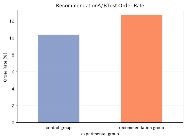
Even if the recommended model has high offline accuracy, displaying it does not necessarily mean more orders. By randomly assigning target customers to control groups and policy groups, and measuring the Incremental effect of order rates, we create the basis for company-wide deployment.

Approach to Analysis and Modeling

If the order acceptance rate for the policy and control groups is $\hat{p}_1,\hat{p}_0$, the absolute effect is $\hat{\Delta}=\hat{p}_1-\hat{p}_0$. Standard error of two independent samples

$SE(\hat{\Delta})=\sqrt{\frac{\hat{p}_1(1-\hat{p}_1)}{n_1}+\frac{\hat{p}_0(1-\hat{p}_0)}{n_0}}$

Find a 95% confidence interval from this. In addition to statistical significance, we check whether incremental gross profit exceeds delivery and implementation costs.

Check with Python

ab = customers.groupby("treatment")["order"].agg(["mean", "sum", "count"])
p0, p1 = ab.loc[0, "mean"], ab.loc[1, "mean"]
n0, n1 = ab.loc[0, "count"], ab.loc[1, "count"]
lift = p1 - p0
se = np.sqrt(p1*(1-p1)/n1 + p0*(1-p0)/n0)
ci = (lift - 1.96*se, lift + 1.96*se)
z = lift / se
p_value = 2 * stats.norm.sf(abs(z))
display(ab.rename(index={0:"control group", 1:"recommendation group"}))
print(f"Order rate difference: {lift:.1%}, 95% CI: [{ci[0]:.1%}, {ci[1]:.1%}], pvalue: {p_value:.4f}")
ax = (ab["mean"]*100).rename(index={0:"control group",1:"recommendation group"}).plot(kind="bar", color=["#8da0cb", "#fc8d62"])
ax.set_title("RecommendationA/BTest Order Rate")
ax.set_xlabel("experimental group")
ax.set_ylabel("Order Rate (%）")
ax.grid(axis="y", alpha=.3)
plt.xticks(rotation=0)
plt.tight_layout()
plt.show()

	mean	sum	count
treatment
control group	0.10	106	1021
recommendation group	0.13	124	979

Order rate difference: 2.3%, 95% CI: [-0.5%, 5.1%], p-value: 0.1099

Reading the results

Check the order rate differences and confidence intervals for each group of initiatives. If the confidence interval exceeds zero, rather than concluding it as “no effect,” consider sample shortages and segment differences. In production judgment, it is safer to use the gate to ensure that the conservative incremental gross profit using the lower limit of the effect exceeds operating costs.

No.072: Recommendation and LTV

Meaning in Practice

Maximizing only the probability of one-off orders may lead to customers who rely on discounts or projects with heavy maintenance burdens. Priority is determined by LTV, including recurring gross profit, and sales man-hours and recommended quotas are allocated to customers with high long-term value.

Approach to Analysis and Modeling

Simplified LTV is calculated as initial gross profit $M_0$, monthly recurring gross profit $m$, monthly recurrence rate $r$, and monthly discount rate $d$

$LTV=M_0+\sum_{t=1}^{T}\frac{m r^t}{(1+d)^t}$

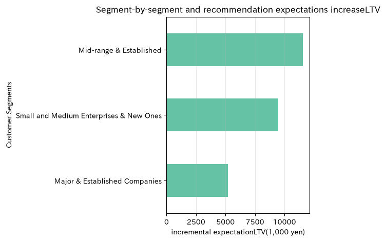
This is how it will be evaluated. The expected value of a recommendation is compared by the incremental LTV of the order probability × from the recommendation.

Check with Python

segment = pd.DataFrame({
    "segment":["Small and Medium Enterprises & New Ones", "Mid-range & Established", "Major & Established Companies"],
    "initial_margin":[90, 150, 240], "monthly_margin":[18, 35, 60],
    "retention":[.88, .94, .97], "uplift":[.050, .035, .020], "eligible":[900, 600, 220]
})
T, discount = 24, .006
segment["LTV"] = segment.apply(lambda r: r.initial_margin + sum(r.monthly_margin*r.retention**t/(1+discount)**t for t in range(1,T+1)), axis=1)
segment["incremental_value"] = segment["LTV"] * segment["uplift"] * segment["eligible"]
display(segment.sort_values("incremental_value", ascending=False))
ax = segment.set_index("segment")["incremental_value"].sort_values().plot(kind="barh", color="#66c2a5")
ax.set_title("Segment-by-segment and recommendation expectations increaseLTV")
ax.set_xlabel("incremental expectationLTV(1,000 yen)")
ax.set_ylabel("Customer Segments")
ax.grid(axis="x", alpha=.3)
plt.tight_layout()
plt.show()

	segment	initial_margin	monthly_margin	retention	uplift	eligible	LTV	incremental_value
1	Mid-range & Established	150	35	0.94	0.04	600	550.68	11,564.24
0	Small and Medium Enterprises & New Ones	90	18	0.88	0.05	900	210.65	9,479.20
2	Major & Established Companies	240	60	0.97	0.02	220	1,182.46	5,202.84

Reading the results

The segment with the largest LTV may not match the segment with the highest incremental value across the entire campaign. The target number and the causal uplift are also combined to allocate sales slots. Since the estimation error in continuity rate can greatly influence results, sensitivity analyses of pessimism, standards, and optimism are also included during operation.

No.073: Application of the Recommendation System to E-commerce

Meaning in Practice

In BtoB e-commerce, ranking is necessary not only based on ease of clicking, but also considering gross margin, inventory, and delivery time. Minimize exposure of out-of-stock products and prioritize alternatives with surplus supply capacity.

Approach to Analysis and Modeling

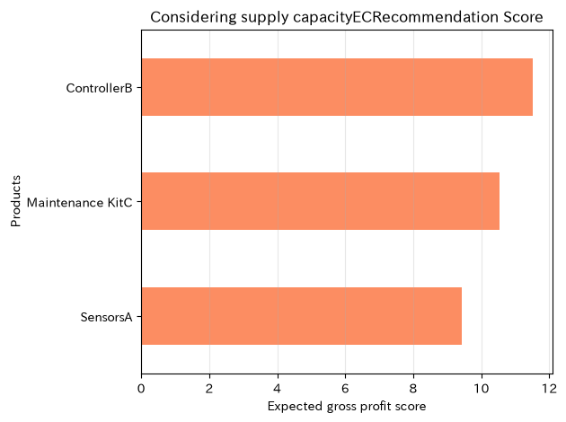
Set the candidate product’s score to Purchase Probability × Gross profit per unit × inventory sufficiency factor. This is a simple expected gross profit ranking. In production, we add customer suitability, contract pricing, compatibility, and out-of-stock penalties.

Check with Python

ec = products.copy()
ec["purchase_prob"] = [.24, .18, .31]
ec["demand_30d"] = [220, 95, 170]
ec["availability"] = np.minimum(1, ec["stock"] / ec["demand_30d"])
ec["recommend_score"] = ec["purchase_prob"] * ec["unit_margin"] * ec["availability"]
ec["rank"] = ec["recommend_score"].rank(ascending=False, method="first").astype(int)
display(ec.sort_values("rank"))
ax = ec.sort_values("recommend_score").plot.barh(x="product", y="recommend_score", legend=False, color="#fc8d62")
ax.set_title("Considering supply capacityECRecommendation Score")
ax.set_xlabel("Expected gross profit score")
ax.set_ylabel("Products")
ax.grid(axis="x", alpha=.3)
plt.tight_layout()
plt.show()

	product	price	unit_margin	stock	purchase_prob	demand_30d	availability	recommend_score	rank
1	ControllerB	210	76	80	0.18	95	0.84	11.52	1
2	Maintenance KitC	75	34	260	0.31	170	1.00	10.54	2
0	SensorsA	120	48	180	0.24	220	0.82	9.43	3

Reading the results

Even if the purchase probability is high, products with low inventory fulfillment rates will rank lower. However, if you conceal supply constraints and constantly lower the number of best-selling items, you may miss demand opportunities, so the “raw score for demand forecasting” and the “restricted score for display” are stored separately.

No.074: Application of the Recommendation System to Manufacturing

Meaning in Practice

Manufacturers are not only recommended for products. Based on equipment operating hours and failure history, you can present replacement parts, inspections, and technical documents as ‘next best actions’ to sales and maintenance staff.

Approach to Analysis and Modeling

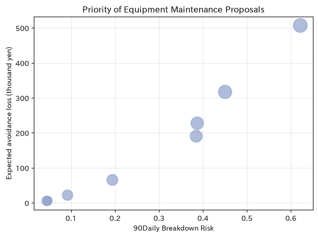
Estimate failure risk and proposal acceptance probability for each piece of equipment, prioritizing Risks × Probability of acceptance × avoidance loss. It is important that essential safety inspections are enforced by rules rather than scoring.

Check with Python

assets = pd.DataFrame({
    "asset":[f"M-{i:02d}" for i in range(1,9)],
    "runtime_h":[8200,4300,6700,9100,3800,7600,5400,8800],
    "fault_count":[3,0,2,5,1,4,1,3],
    "accept_prob":[.55,.20,.45,.68,.25,.60,.35,.64],
    "avoided_loss":[900,600,750,1200,500,980,680,1100]
})
logit = -5 + .00045*assets.runtime_h + .28*assets.fault_count
assets["failure_risk"] = 1/(1+np.exp(-logit))
assets["priority_value"] = assets.failure_risk*assets.accept_prob*assets.avoided_loss
display(assets.sort_values("priority_value", ascending=False).head())
ax = assets.plot.scatter(x="failure_risk", y="priority_value", s=assets["avoided_loss"]/3, alpha=.7, color="#8da0cb")
ax.set_title("Priority of Equipment Maintenance Proposals")
ax.set_xlabel("90Daily Breakdown Risk")
ax.set_ylabel("Expected avoidance loss (thousand yen)")
ax.grid(alpha=.3)
plt.tight_layout()
plt.show()

	asset	runtime_h	fault_count	accept_prob	avoided_loss	failure_risk	priority_value
3	M-04	9100	5	0.68	1200	0.62	506.97
7	M-08	8800	3	0.64	1100	0.45	316.92
5	M-06	7600	4	0.60	980	0.39	227.55
0	M-01	8200	3	0.55	900	0.38	190.39
2	M-03	6700	2	0.45	750	0.19	65.43

Reading the results

By including not only failure risks but also acceptability and avoidable losses, it becomes clear which equipment personnel should contact first. For equipment with high risk and low acceptance, technical explanations and joint planning of shutdown plans may be more appropriate than discounts.

No.075: Integration of recommendation systems and AI agents

Meaning in Practice

AI agents can link candidate selection, inventory inquiries, and caption creation. On the other hand, automatically sending messages such as compatibility violations, contract deviations, or supply failures can cause significant damage, so authorization boundaries are necessary.

Approach to Analysis and Modeling

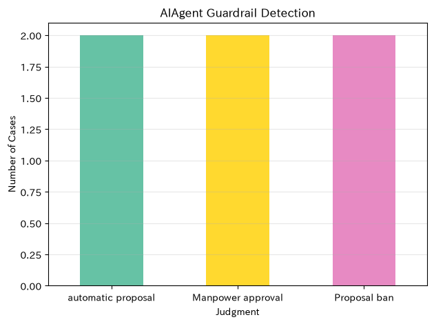
In addition to the forecast score, policies are determined based on inventory, compatibility, reliability, and deal amount. Here, we simulate a design that divides the process into three stages: “automatic proposal,” “manual approval,” and “proposal prohibition,” and keeps a decision log.

Check with Python

agent_cases = pd.DataFrame({
    "case":["Q-101","Q-102","Q-103","Q-104","Q-105","Q-106"],
    "score":[.88,.77,.91,.63,.82,.72], "confidence":[.92,.61,.95,.86,.74,.89],
    "stock_ok":[True,True,False,True,True,True], "compatible":[True,True,True,False,True,True],
    "deal_value":[180,2400,350,220,480,900]
})
def policy(r):
    if not r.stock_ok or not r.compatible: return "Proposal ban"
    if r.confidence < .8 or r.deal_value >= 1000: return "Manpower approval"
    return "automatic proposal"
agent_cases["decision"] = agent_cases.apply(policy, axis=1)
display(agent_cases)
counts = agent_cases["decision"].value_counts().reindex(["automatic proposal","Manpower approval","Proposal ban"], fill_value=0)
ax = counts.plot(kind="bar", color=["#66c2a5","#ffd92f","#e78ac3"])
ax.set_title("AIAgent Guardrail Detection")
ax.set_xlabel("Judgment")
ax.set_ylabel("Number of Cases")
ax.grid(axis="y", alpha=.3)
plt.xticks(rotation=0)
plt.tight_layout()
plt.show()

	case	score	confidence	stock_ok	compatible	deal_value	decision
0	Q-101	0.88	0.92	True	True	180	automatic proposal
1	Q-102	0.77	0.61	True	True	2400	Manpower approval
2	Q-103	0.91	0.95	False	True	350	Proposal ban
3	Q-104	0.63	0.86	True	False	220	Proposal ban
4	Q-105	0.82	0.74	True	True	480	Manpower approval
5	Q-106	0.72	0.89	True	True	900	automatic proposal

Reading the results

Even with high scores, out-of-stock or compatibility violations will be prohibited from proposals. By redirecting high-value and low-trust projects to manual approval, you can achieve both efficiency and control. In operations, input data, candidates, reference information, final decisions, and approvers are stored as audit logs.

No.076: Linear Programming

Meaning in Practice

When demand exceeds capacity, relying solely on profit margins cannot properly handle bottlenecks across multiple processes. Using linear programming, production volumes for each product are determined simultaneously.

Approach to Analysis and Modeling

$x_j$ the production volume of the product $j$ and use marginal profit as the $c_j$ to solve $\max \sum_j c_jx_j$. If the equipment $i$ is $a_{ij}$ the usage coefficient and the capacity is $b_i$, it is $\sum_j a_{ij}x_j\le b_i$. We assume material and bulk production capable of handling continuous volumes.

Check with Python

lp_products = ["IngredientsA","IngredientsB","IngredientsC"]
margin = np.array([42, 55, 38])
A = np.array([[2.0, 3.0, 1.5], [1.0, .8, 1.6]])
capacity = np.array([720, 360])
demand = np.array([180, 140, 200])
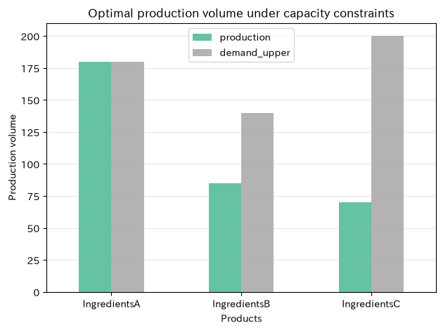
res_lp = linprog(-margin, A_ub=A, b_ub=capacity, bounds=list(zip(np.zeros(3), demand)), method="highs")
lp_plan = pd.DataFrame({"product":lp_products, "production":res_lp.x, "demand_upper":demand, "unit_margin":margin})
display(lp_plan)
print(f"maximum marginal profit: {-res_lp.fun:,.1f} thousand yen")
ax = lp_plan.plot.bar(x="product", y=["production","demand_upper"], color=["#66c2a5","#b3b3b3"])
ax.set_title("Optimal production volume under capacity constraints")
ax.set_xlabel("Products")
ax.set_ylabel("Production volume")
ax.grid(axis="y", alpha=.3)
plt.xticks(rotation=0)
plt.tight_layout()
plt.show()

	product	production	demand_upper	unit_margin
0	IngredientsA	180.00	180	42
1	IngredientsB	85.00	140	55
2	IngredientsC	70.00	200	38

Maximum Profit Margin: 14,895.0 thousand yen

Reading the results

Products are divided into those that are made up to the demand ceiling and those that are limited by capability constraints. Even products with high unit profit margins may not be prioritized if they consume more bottlenecks. In practice, along with solutions, we check constraints and shadow prices, and evaluate the value of overtime and facility upgrades.

No.077: Integer Programming

Meaning in Practice

Starting up and setting up the production line is a discrete decision on whether to proceed, and fractional solutions for continuous quantities cannot be executed. An integer plan including fixed setup costs and minimum lot sizes is required.

Approach to Analysis and Modeling

We use the number of production lots $x_j$ and the operating status $y_j\in\{0,1\}$, and represent the logical relationship with $x_j\le M_jy_j$ and $x_j\ge L_jy_j$. The objective function subtracts the fixed setup cost from the gross profit per lot.

Check with Python

# Variable order: x_A, x_B, x_C (number of integer lots), y_A, y_B, y_C (binary value)
lot_margin = np.array([110, 145, 95])
setup_cost = np.array([80, 120, 55])
c = np.r_[-lot_margin, setup_cost]
max_lots, min_lots = np.array([8,6,10]), np.array([2,2,3])
rows, ub = [], []
rows.append(np.r_[[3,4,2], [0,0,0]]); ub.append(28)
for j in range(3):
    row = np.zeros(6); row[j]=1; row[3+j]=-max_lots[j]; rows.append(row); ub.append(0)
    row = np.zeros(6); row[j]=-1; row[3+j]=min_lots[j]; rows.append(row); ub.append(0)
res_milp = milp(c, integrality=np.ones(6), bounds=Bounds(np.zeros(6), np.r_[max_lots, np.ones(3)]), constraints=LinearConstraint(np.array(rows), -np.inf, np.array(ub)))
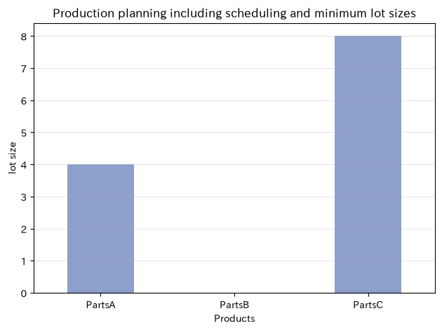
milp_plan = pd.DataFrame({"product":["PartsA","PartsB","PartsC"], "lots":np.rint(res_milp.x[:3]).astype(int), "setup":np.rint(res_milp.x[3:]).astype(int)})
display(milp_plan)
print(f"Profit after setup cost deduction: {-res_milp.fun:,.0f} thousand yen")
ax = milp_plan.plot.bar(x="product", y="lots", legend=False, color="#8da0cb")
ax.set_title("Production planning including scheduling and minimum lot sizes")
ax.set_xlabel("Products")
ax.set_ylabel("lot size")
ax.grid(axis="y", alpha=.3)
plt.xticks(rotation=0)
plt.tight_layout()
plt.show()

	product	lots	setup
0	PartsA	4	1
1	PartsB	0	0
2	PartsC	8	1

Profit after setup expense deduction: 1,065 thousand yen

Reading the results

Because of the setup cost, the solution of consolidating all varieties into a limited variety is chosen rather than a plan to produce all varieties in small quantities. Solutions in integer programming are sensitive to input conditions. We confirm the minimum lot size, changeover time, and delivery deadline with the on-site manager, and in addition to the optimal solution, we also propose alternative solutions with smaller profit margins.

No.078: Inventory Optimization

Meaning in Practice

Uniformly stockpiling safety stock increases working capital, while too little causes shortages. Decide the order points for each item based on demand fluctuations, procurement lead times, and required service levels.

Approach to Analysis and Modeling

If the average daily demand is $\mu_d$, the standard deviation is $\sigma_d$, lead time is $L$ days, and the standard normal quantile corresponding to service level is $z$, then the safety stock and ordering points assuming independent and homogeneous distribution are

$SS=z\sigma_d\sqrt{L},\qquad ROP=\mu_dL+SS$

That’s right. If there is strong seasonal or lead time variation, we replace them with prediction error distributions or simulations.

Check with Python

inventory = pd.DataFrame({
    "item":["SensorsA","ControllerB","Maintenance KitC"],
    "daily_mean":[8.0,3.2,10.5], "daily_std":[2.4,1.4,3.1],
    "lead_time":[12,20,7], "service_level":[.95,.98,.95]
})
inventory["z"] = stats.norm.ppf(inventory.service_level)
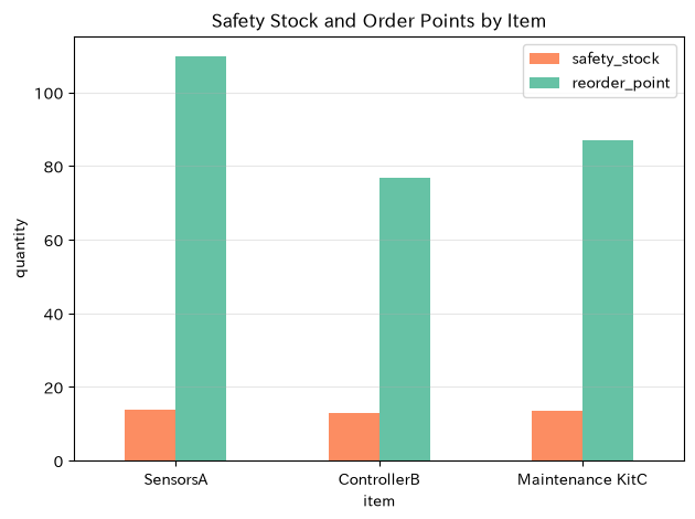
inventory["safety_stock"] = inventory.z*inventory.daily_std*np.sqrt(inventory.lead_time)
inventory["reorder_point"] = inventory.daily_mean*inventory.lead_time + inventory.safety_stock
display(inventory.round(1))
ax = inventory.plot.bar(x="item", y=["safety_stock","reorder_point"], color=["#fc8d62","#66c2a5"])
ax.set_title("Safety Stock and Order Points by Item")
ax.set_xlabel("item")
ax.set_ylabel("quantity")
ax.grid(axis="y", alpha=.3)
plt.xticks(rotation=0)
plt.tight_layout()
plt.show()

	item	daily_mean	daily_std	lead_time	service_level	z	safety_stock	reorder_point
0	SensorsA	8.00	2.40	12	1.00	1.60	13.70	109.70
1	ControllerB	3.20	1.40	20	1.00	2.10	12.90	76.90
2	Maintenance KitC	10.50	3.10	7	1.00	1.60	13.50	87.00

Reading the results

Not only average demand but also fluctuations, lead times, and service levels influence the order point. To set a high service level for expensive controllers, you need grounds for out-of-stock losses and inventory costs. In practice, you also add MOQ, order dates, substitutes, and demand autocorrelation.

No.079: Supply Chain Optimization

Meaning in Practice

When supplying from multiple factories to multiple locations, simply selecting the nearest factory individually can sometimes exceed the factory’s capacity. Seek allocations that meet demand while minimizing overall transportation costs.

Approach to Analysis and Modeling

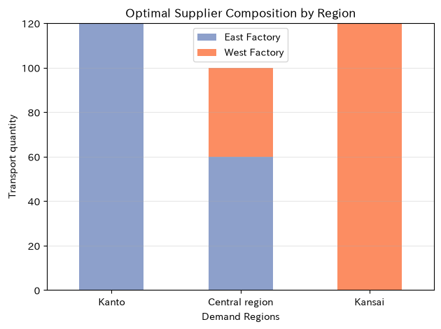
$x_{ij}$ the transportation volume from the factory $i$ to the demand $j$, $c_{ij}$ unit transportation costs, and solve $\min\sum_{ij}c_{ij}x_{ij}$. This is a transportation issue that constrains the supply limits of each factory and the fulfillment of demand at each demand location.

Check with Python

factories, regions = ["East Factory","West Factory"], ["Kanto","Central region","Kansai"]
cost = np.array([[4,6,9],[8,5,3]], dtype=float)
supply, region_demand = np.array([180,160]), np.array([120,100,120])
# The demand constraint is denoted as -sum_i x_ij < = -demand
A_ub, b_ub = [], []
for i in range(2):
    row=np.zeros(6); row[i*3:(i+1)*3]=1; A_ub.append(row); b_ub.append(supply[i])
for j in range(3):
    row=np.zeros(6); row[j]=-1; row[3+j]=-1; A_ub.append(row); b_ub.append(-region_demand[j])
res_ship = linprog(cost.ravel(), A_ub=np.array(A_ub), b_ub=np.array(b_ub), bounds=(0,None), method="highs")
ship = pd.DataFrame(res_ship.x.reshape(2,3), index=factories, columns=regions)
display(ship)
print(f"Minimum transportation cost: {res_ship.fun:,.0f} thousand yen")
ax = ship.T.plot(kind="bar", stacked=True, color=["#8da0cb","#fc8d62"])
ax.set_title("Optimal Supplier Composition by Region")
ax.set_xlabel("Demand Regions")
ax.set_ylabel("Transport quantity")
ax.grid(axis="y", alpha=.3)
plt.xticks(rotation=0)
plt.tight_layout()
plt.show()

	Kanto	Central region	Kansai
East Factory	120.00	60.00	0.00
West Factory	0.00	40.00	120.00

Minimum transportation fee: 1,400 thousand yen

Reading the results

While prioritizing short-distance supply, some areas are supplemented by other plants due to factory capacity limitations. Since the minimum cost solution alone is vulnerable to disaster and outage risks, in practice, double procurement ratios, CO2, delivery dates, and BCP inventory are added to constraints or objective functions.

No.080: Marketing Budget Allocation

Meaning in Practice

Decide how to allocate limited budgets for exhibitions, search ads, existing customer seminars, and sales support. If you invest all your money in initiatives with high average ROI, you ignore saturation and channel dependency.

Approach to Analysis and Modeling

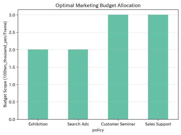
Each initiative is divided into investment limits in units of 1,000,000 yen, and the marginal gross profit decreases as the limit advances. Using 0-1 variables for each selected slot, the total budget, policy cap, and minimum necessary brand initiatives are constrained to maximize incremental gross profit.

Check with Python

channels = ["Exhibition","Search Ads","Customer Seminar","Sales Support"]
returns = {
    "Exhibition":[1.9,1.5,1.1,0.8], "Search Ads":[2.2,1.6,1.0,0.6],
    "Customer Seminar":[2.5,1.9,1.4,1.0], "Sales Support":[2.1,1.8,1.5,1.2]
}
items=[(ch,k,r) for ch in channels for k,r in enumerate(returns[ch], start=1)]
# 10 slots (1 slot = 1,000,000 yen), with at least one slot for exhibitions. Since it's a deductible line, it is naturally selected from the previous slot.
c=-np.array([r for _,_,r in items])
budget_row=np.ones(len(items))
expo_row=np.array([-1 if ch=="Exhibition" else 0 for ch,_,_ in items])
res_budget=milp(c, integrality=np.ones(len(items)), bounds=Bounds(np.zeros(len(items)),np.ones(len(items))), constraints=LinearConstraint(np.vstack([budget_row,expo_row]),[-np.inf,-np.inf],[10,-1]))
chosen=np.rint(res_budget.x).astype(int)
allocation=pd.DataFrame(items,columns=["channel","block","incremental_margin"])
allocation["selected"]=chosen
summary=allocation.query("selected==1").groupby("channel").agg(budget_blocks=("selected","sum"), expected_margin=("incremental_margin","sum")).reindex(channels,fill_value=0)
display(summary)
print(f"allocation budget: {summary.budget_blocks.sum()*100:,.0f} ten_thousand_yen, Expected Incremental Gross Profit Index: {summary.expected_margin.sum():.1f}")
ax = summary["budget_blocks"].plot(kind="bar", color="#66c2a5")
ax.set_title("Optimal Marketing Budget Allocation")
ax.set_xlabel("policy")
ax.set_ylabel("Budget Scope (100ten_thousand_yen/Frame)")
ax.grid(axis="y", alpha=.3)
plt.xticks(rotation=0)
plt.tight_layout()
plt.show()

	budget_blocks	expected_margin
channel
Exhibition	2	3.40
Search Ads	2	3.80
Customer Seminar	3	5.80
Sales Support	3	5.40

Allocation budget: 10 million yen, Expected incremental gross profit index: 18.4

Reading the results

Since you select from the slots with the highest marginal effect, the budget is spread across multiple initiatives. This is not a uniform distribution but a result based on the diminishing effect. Coefficients are not simply based on ROI from observational data, but are estimated through experiments and MMM by region and period, and sales capacity and lead quality are also included as constraints.

Practical Implications Seen Through Target Exercise

1. From recommendation accuracy to incremental value: Measure causal effects through A/B testing and convert them into policy value using LTV and gross profit.
2. Connecting demand creation and supply constraints: Inventory availability, delivery times, and compatibility are reflected in the display rankings for e-commerce and sales.
3. Separating Forecasting and Decision-Making: Demand and order probabilities are handled by the forecasting model, while allocation is handled by the optimization model. Records both inputs and outputs.
4. Set rejection conditions for automation: AI agents can be safely used by returning high-cost, low-trust, and rule-violating cases back to humans.
5. Don’t overestimate the optimal solution for a single point: Compare sensitivity analyses and alternative solutions that vary demand, effectiveness, and cost.

What is necessary for practical implementation

• Standardize IDs and update times for customers, products, inventory, capacity, and costs.
• KPIs are defined not only by order rate but also by incremental gross profit, LTV, out-of-stock rate, and on-time delivery rate.
• Pre-register the experimental unit, required sample quantity, and stop criteria
• Inventory optimization constraints and exception rules with the field and assign responsible persons
• Enable auditability of recommendation reasons, input data, model versions, and approval results
• Deploy in the order of small-scale PoCs, parallel operation, and limited automation.

Conclusion

In No.071 to No.080, recommendations were not limited to “techniques that produce easy candidates,” but rather by confirming incremental value through experiments, evaluating customers’ long-term value, and finding ways to implement feasible plans under supply constraints. The key to achieving results in manufacturing lies not in the sophistication of individual models, but in connecting demand, supply, profit, and control to the same decision-making process.

Consultations for Corporations

At Suri Kobo, we support everything from problem organization, data design, PoC, on-site implementation, to in-house training, covering recommendations, demand forecasting, inventory, production, logistics, and marketing allocation. We work together from an environment that can be explained and operated, taking into account existing systems and on-site rules.

📩 Contact Us: surikobo.co.jp/contact Please feel free to consult us first.