Price Optimization of Industrial Filters: From Demand Response to Continued Operation (No.051–No.060)

This article focuses on a fictional manufacturing industry that handles industrial dust filters, covering price elasticity, customer preferences, profit maximization, dynamic pricing, promotions and coupons, online learning, Bayesian optimization, reinforcement learning, and practical implementation as a single decision-making process. The goal is not to consider prices solely by the “degree of increase,” but to simultaneously consider demand, gross profit, production capacity, customer relationships, and learning costs.

[!NOTE] This material is a notebook previously used by Surikoubo (or personally by the representative, Kazuyama), and has been reconstructed, edited, and published with the company’s permission. All data listed is fictional and has no relation whatsoever to real companies, factories, or figures.

Introduction: Practical Challenges in Manufacturing Covered in This Article

While raw material and logistics costs are rising, the sales department is worried about losing orders. Furthermore, there are months when production capacity is tight and months when there is margin, and simply quoting the same price for all customers and all periods misses profit opportunities. In this article, we will create a minimum structure where sales, production, and accounting can discuss prices using common values.

Common situations on site

• Quantity decreases after price hikes are based solely on experience.
• Policies that pursue sales and those that pursue marginal profit are mixed together.
• The discount is ‘carried over from last year,’ and the incremental profit has not been verified.
• Customer pricing becomes personalized and learning outcomes do not remain with the organization.
• Even if demand is stimulated, factory supply capacity becomes a bottleneck.

Why is this issue so difficult to judge?

Prices move demand and gross profit in opposite directions. Also, since observational data mixes customer composition, seasons, and sales efforts, the correlation between price and order volume cannot be considered directly causal. Not only short-term profits but also long-term contracts, explainability, fairness, and brand damage are constrained.

Overview of Exercise covered this time

In No.051 to No.053, you will learn about price responses and static profit maximization, while in No.054 to No.056, you will handle differences in timing, promotions, and customers. No.057 to No.059 compare methods of learning during operations and integrate them into implementation plans including KPIs, approvals, and monitoring in No.060.

Preparing the Python environment

No external data is used. Fix the random number generator so you can reproduce the same results. Unless otherwise specified, amounts are in yen, and quantities are per piece per month.

import sys
import numpy as np
import pandas as pd
import matplotlib
import matplotlib.pyplot as plt
import japanize_matplotlib
from scipy.optimize import minimize_scalar
from sklearn.linear_model import LinearRegression

SEED = 20260712
rng = np.random.default_rng(SEED)
pd.set_option("display.float_format", lambda x: f"{x:,.2f}")
print(f"Python {sys.version.split()[0]} / pandas {pd.__version__} / matplotlib {matplotlib.__version__}")

Python 3.13.1 / pandas 3.0.3 / matplotlib 3.11.0

Creation of Fictional Data

Generate business negotiation data for 3 customer segments over 24 months. Prices fluctuate depending on market conditions and monthly, while demand is influenced by price, seasonality, and customer size. The true demand formula is used only for generating data for the teaching materials, while the analysis side estimates it from observational data.

months = pd.date_range("2024-01-01", periods=24, freq="MS")
segments = {"large mouth": (320, -1.15), "backbone": (190, -1.55), "small mouth": (95, -2.05)}
rows = []
for t, month in enumerate(months):
    season = 1 + 0.10 * np.sin(2 * np.pi * t / 12)
    market = 1 + 0.025 * t / 12
    for segment, (base_qty, elasticity) in segments.items():
        price = 10_000 * market * rng.uniform(0.92, 1.10)
        expected = base_qty * season * (price / 10_000) ** elasticity
        quantity = max(1, int(round(expected + rng.normal(0, base_qty * 0.045))))
        rows.append((month, segment, price, quantity, 6_200 + 18 * t))
sales = pd.DataFrame(rows, columns=["month", "segment", "price", "quantity", "unit_cost"])
sales["revenue"] = sales.price * sales.quantity
sales["gross_profit"] = (sales.price - sales.unit_cost) * sales.quantity
display(sales.head(6))
print(f"Number of lines: {len(sales):,}, Sales: {sales.revenue.sum()/1e6:,.1f}million yen")

	month	segment	price	quantity	unit_cost	revenue	gross_profit
0	2024-01-01	large mouth	10,446.52	314	6200	3,280,205.73	1,333,405.73
1	2024-01-01	backbone	10,764.81	168	6200	1,808,488.43	766,888.43
2	2024-01-01	small mouth	9,260.98	113	6200	1,046,490.19	345,890.19
3	2024-02-01	large mouth	10,916.25	300	6218	3,274,875.57	1,409,475.57
4	2024-02-01	backbone	9,544.64	228	6218	2,176,176.96	758,472.96
5	2024-02-01	small mouth	9,751.53	105	6218	1,023,911.01	371,021.01

Number of lines: 72, Sales: 144.8 million yen

No.051: Price Elasticity

Meaning in Practice

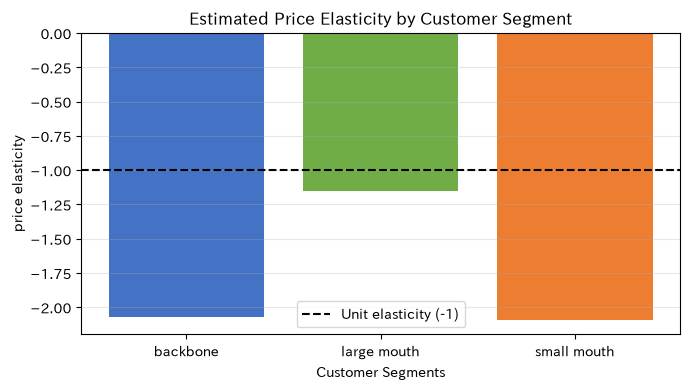
Price elasticity represents how much demand changes when the price changes by 1%. In markets where the absolute value exceeds 1, demand reacts strongly to price changes. However, price increases are not determined solely by elasticity; costs and capability constraints are also considered.

Approach to Analysis and Modeling

Let the constant elasticity model be $Q=A P^{\varepsilon}$, then take the logarithm and

$\log Q=\alpha+\varepsilon\log P$

The regression coefficient $\varepsilon$ represents price elasticity. Here, a monthly dummy is also added to minimize the impact of seasonal fluctuations. Since endogeneity remains in observational studies, price experiments and manipulative variables are also considered in production.

Check with Python

elasticity_rows = []
for segment, g in sales.groupby("segment"):
    X = pd.concat([np.log(g.price).rename("log_price"), pd.get_dummies(g.month.dt.month, prefix="m", drop_first=True)], axis=1)
    model = LinearRegression().fit(X, np.log(g.quantity))
    elasticity_rows.append((segment, model.coef_[0], model.score(X, np.log(g.quantity))))
elasticity_df = pd.DataFrame(elasticity_rows, columns=["segment", "estimated_elasticity", "R2"])
display(elasticity_df)

fig, ax = plt.subplots(figsize=(7, 4))
ax.bar(elasticity_df.segment, elasticity_df.estimated_elasticity, color=["#4472C4", "#70AD47", "#ED7D31"])
ax.axhline(-1, color="black", linestyle="--", label="Unit elasticity (-1)")
ax.set_title("Estimated Price Elasticity by Customer Segment")
ax.set_xlabel("Customer Segments"); ax.set_ylabel("price elasticity")
ax.grid(axis="y", alpha=.3); ax.legend(); plt.tight_layout(); plt.show()

	segment	estimated_elasticity	R2
0	backbone	-2.07	0.96
1	large mouth	-1.15	0.98
2	small mouth	-2.09	0.93

Reading the results

The smaller the portion, the larger the absolute value, which makes price comparisons more likely to occur, which is also considered a regression setting. For large traders, value propositions including supply stability and technical support are important, rather than uniform discounts; for small traders, monitoring competitive prices is important. Estimates are used for decision-making after reviewing the target period, confidence intervals, and pricing process.

No.052: Conjoint Analysis

Meaning in Practice

For B2B products, not only unit price but also lifespan, delivery time, and maintenance contracts influence selection. Conjoint analysis is a method where customers estimate the relative value of each attribute from selection data comparing the entire product, and design specifications and pricing simultaneously.

Approach to Analysis and Modeling

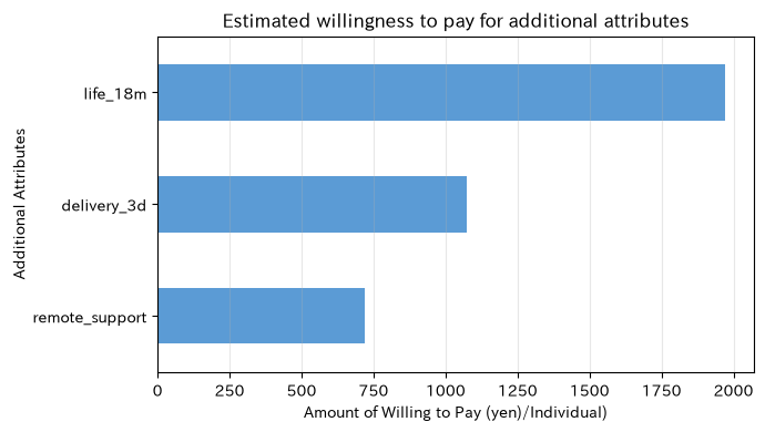
Set utility to $U=\beta_0+\beta_p P+\sum_k\beta_k x_k$, and this time, we will check partial utility using linear regression from a hypothetical choice score. The willingness to pay for an attribute is calculated by dividing the attribute coefficient by the absolute value of the price coefficient. For discrete selection in production, the Logit model and hierarchical Bayes are suitable.

Check with Python

n = 240
profiles = pd.DataFrame({
    "price_k": rng.choice([9.5, 10.5, 11.5, 12.5], n),
    "life_18m": rng.integers(0, 2, n),
    "delivery_3d": rng.integers(0, 2, n),
    "remote_support": rng.integers(0, 2, n),
})
true_beta = np.array([-0.85, 1.50, 0.95, 0.65])
profiles["preference_score"] = profiles[["price_k", "life_18m", "delivery_3d", "remote_support"]].to_numpy() @ true_beta + rng.normal(0, .65, n)
conjoint = LinearRegression().fit(profiles.drop(columns="preference_score"), profiles.preference_score)
coef = pd.Series(conjoint.coef_, index=profiles.columns[:-1], name="partial utility")
wtp = (coef.drop("price_k") / abs(coef["price_k"]) * 1000).rename("amount_of_willing_to_pay_yen")
display(pd.concat([coef, wtp], axis=1))

fig, ax = plt.subplots(figsize=(7, 4))
wtp.sort_values().plot.barh(ax=ax, color="#5B9BD5")
ax.set_title("Estimated willingness to pay for additional attributes")
ax.set_xlabel("Amount of Willing to Pay (yen)/Individual)"); ax.set_ylabel("Additional Attributes")
ax.grid(axis="x", alpha=.3); plt.tight_layout(); plt.show()

	partial utility	amount_of_willing_to_pay_jpy
price_k	-0.81	NaN
life_18m	1.60	1,972.24
delivery_3d	0.87	1,074.14
remote_support	0.59	720.21

Reading the results

The largest willingness to pay for longevity is the most significant, followed by short delivery times and remote support. Attributes where the additional cost is less than the willingness to pay are candidates for the high value-added version. However, since average values alone can hide differences in customers, design and analyze by purchasing participants and specific use cases.

No.053: Maximizing Profit

Meaning in Practice

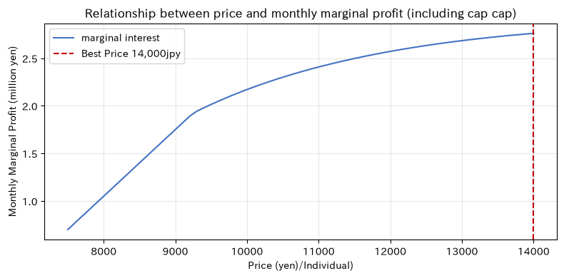
Maximizing sales and maximizing profits do not coincide. Lowering the price increases quantity, but the marginal profit per unit shrinks. By connecting demand forecasts by price with costs, we visualize sensitivity to operating profit.

Approach to Analysis and Modeling

If we $Q(P)=A(P/P_0)^\varepsilon$ forecasted demand and unit variable cost $c$, the marginal profit is

$\Pi(P)=(P-c)Q(P)$

That’s right. Here, the cap is also included, and the available quantity is set at $\min(Q(P),K)$.

Check with Python

price_grid = np.arange(7_500, 14_001, 100)
base_demand, base_price, eps, unit_cost, capacity = 620, 10_000, -1.55, 6_500, 700
demand = base_demand * (price_grid / base_price) ** eps
sold = np.minimum(demand, capacity)
profit = (price_grid - unit_cost) * sold
profit_table = pd.DataFrame({"price": price_grid, "demand": demand, "sold": sold, "gross_profit": profit})
best = profit_table.loc[profit_table.gross_profit.idxmax()]
display(best.to_frame("optimal point"))

fig, ax = plt.subplots(figsize=(8, 4))
ax.plot(price_grid, profit / 1e6, label="marginal interest", color="#4472C4")
ax.axvline(best.price, color="#C00000", linestyle="--", label=f"Best Price {best.price:,.0f}jpy")
ax.set_title("Relationship between price and monthly marginal profit (including cap cap)")
ax.set_xlabel("Price (yen)/Individual)"); ax.set_ylabel("Monthly Marginal Profit (million yen)")
ax.grid(alpha=.3); ax.legend(); plt.tight_layout(); plt.show()

	optimal point
price	14,000.00
demand	368.04
sold	368.04
gross_profit	2,760,288.64

Reading the results

The area near the peak of the profit curve is relatively flat, so there is little reason to stick to the “one-point optimum” in tens of yen increments. On site, it is more reliable to set acceptable price ranges and choose adoption prices by considering competitors, contracts, capabilities, and estimation errors.

No.054: Dynamic Pricing

Meaning in Practice

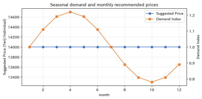
If demand and production capacity differ month by month, fixed prices cause missed opportunities. However, rather than arbitrarily changing existing contracts, design them as explainable pricing rules such as spot orders, short delivery fees, and off-peak discounts.

Approach to Analysis and Modeling

Forecast demand coefficient $A_t$ and capacity $K_t$ at $t$ each month, and select $\max_p (p-c_t)\min\{Q_t(p),K_t\}$ from the candidate price. If carrying over to the future or inventory is important, extend to multi-period optimization.

Check with Python

dynamic_rows = []
for t in range(12):
    season = 1 + .22 * np.sin(2 * np.pi * t / 12)
    cap = 650 + 70 * np.cos(2 * np.pi * t / 12)
    cost = 6_500 + 120 * np.sin(2 * np.pi * (t + 2) / 12)
    q = 620 * season * (price_grid / 10_000) ** -1.55
    gp = (price_grid - cost) * np.minimum(q, cap)
    i = np.argmax(gp)
    dynamic_rows.append((t + 1, season, cap, price_grid[i], gp[i]))
dynamic = pd.DataFrame(dynamic_rows, columns=["month", "demand_index", "capacity", "optimal_price", "gross_profit"])
display(dynamic.round(1))

fig, ax1 = plt.subplots(figsize=(8, 4))
ax1.plot(dynamic.month, dynamic.optimal_price, marker="o", color="#4472C4", label="Suggested Price")
ax1.set_xlabel("month"); ax1.set_ylabel("Suggested Price (Yen)/Individual)")
ax2 = ax1.twinx(); ax2.plot(dynamic.month, dynamic.demand_index, marker="s", color="#ED7D31", label="Demand Index")
ax2.set_ylabel("Demand Index")
ax1.set_title("Seasonal demand and monthly recommended prices"); ax1.grid(alpha=.3)
lines = ax1.lines + ax2.lines; ax1.legend(lines, [x.get_label() for x in lines], loc="best")
plt.tight_layout(); plt.show()

	month	demand_index	capacity	optimal_price	gross_profit
0	1	1.00	720.00	14000	2,722,041.00
1	2	1.10	710.60	14000	3,014,897.70
2	3	1.20	685.00	14000	3,240,659.40
3	4	1.20	650.00	14000	3,340,611.70
4	5	1.20	615.00	14000	3,286,194.30
5	6	1.10	589.40	14000	3,088,431.80
6	7	1.00	580.00	14000	2,798,536.30
7	8	0.90	589.40	14000	2,495,963.40
8	9	0.80	615.00	14000	2,265,343.50
9	10	0.80	650.00	14000	2,170,249.30
10	11	0.80	685.00	14000	2,234,383.00
11	12	0.90	710.60	14000	2,437,003.60

Reading the results

In months with strong demand, the suggested price increases, and we adjust the price to compensate for missed items due to capacity shortages. In practice, constraints such as price change frequency, upper and lower limits, and advance notification to customers are set as constraints, leaving behind understandable reasons such as emergency response compensation.

No.055: Campaign Optimization

Meaning in Practice

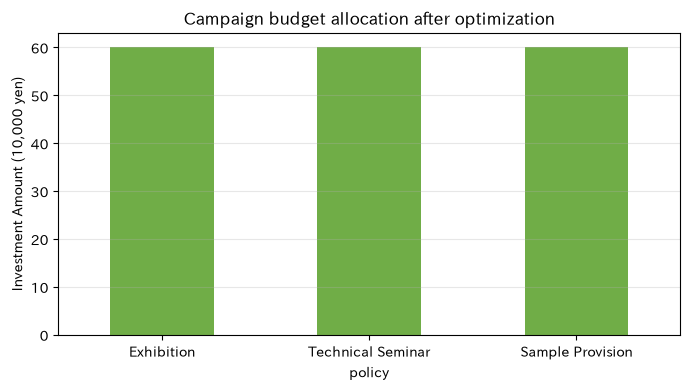
Exhibitions, technical seminars, and sample provision use not only budget but also the man-hours of sales and technical staff. Allocation to the channel is determined based on incremental marginal profit rather than response rate.

Approach to Analysis and Modeling

Let the number of units $j$ be $x_j$, and the marginal incremental profit be the decreasing function $g_j(x_j)$. Maximize $\sum_j g_j(x_j)-c_jx_j$ within the total budget. To make it easier to understand, we allocate 100,000 yen in units using the greedy method.

Check with Python

channels = {"Exhibition": (95, .16), "Technical Seminar": (72, .12), "Sample Provision": (58, .09)}  # Initial incremental profit (10,000 yen), decay rate
budget_units = 18
allocation = {k: 0 for k in channels}
gain = {k: 0.0 for k in channels}
for _ in range(budget_units):
    marginal = {k: a * np.exp(-d * allocation[k]) for k, (a, d) in channels.items()}
    chosen = max(marginal, key=marginal.get)
    allocation[chosen] += 1; gain[chosen] += marginal[chosen]
campaign = pd.DataFrame({"investment_amount_ten_thousand_yen": {k: v * 10 for k, v in allocation.items()}, "incremental_marginal_profit_ten_thousand_yen": gain})
campaign["ROI"] = campaign.incremental_marginal_profit_ten_thousand_yen / campaign.investment_amount_ten_thousand_yen
display(campaign)

fig, ax = plt.subplots(figsize=(7, 4))
campaign.investment_amount_ten_thousand_yen.plot.bar(ax=ax, color="#70AD47")
ax.set_title("Campaign budget allocation after optimization")
ax.set_xlabel("policy"); ax.set_ylabel("Investment Amount (10,000 yen)")
ax.grid(axis="y", alpha=.3); plt.xticks(rotation=0); plt.tight_layout(); plt.show()

	investment_amount_ten_thousand_yen	incremental_marginal_profit_ten_thousand_yen	ROI
Exhibition	60	396.50	6.61
Technical Seminar	60	326.80	5.45
Sample Provision	60	281.18	4.69

Reading the results

Rather than allocating the entire amount to a single measure based solely on initial efficiency, the marginal effects after diminishing are allocated to balance out. It is important that the coefficients are updated as incremental effects through experiments divided by region or customer group, rather than past correlations.

No.056: Coupon Design

Meaning in Practice

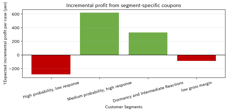
B2B coupons can be used for initial orders for maintenance parts, resuming dormant customers, transitioning to online ordering, and more. Incremental profit is evaluated including discounted existing demand (cannibalization).

Approach to Analysis and Modeling

Incremental profit from issuing coupons to customer $i$

$\Delta\Pi_i=(p-d-c)\Pr(Y_i(1)=1)-(p-c)\Pr(Y_i(0)=1)$

Let’s say so. After deducting distribution costs, only positive customers are targeted. In practice, we estimate two probability differences using the uplift model and randomized controlled trials.

Check with Python

coupon = pd.DataFrame({
    "segment": ["High probability, low response", "Medium probability, high response", "Dormancy and Intermediate Reactions", "low gross margin"],
    "p_without": [.72, .35, .08, .28], "p_with": [.76, .58, .22, .50],
    "price": [10_500, 10_500, 10_500, 8_000], "cost": [6_200, 6_200, 6_200, 6_900],
    "discount": [500, 500, 700, 500], "contact_cost": [80, 80, 120, 80],
})
coupon["incremental_profit"] = ((coupon.price-coupon.discount-coupon.cost)*coupon.p_with
                                - (coupon.price-coupon.cost)*coupon.p_without-coupon.contact_cost)
coupon["send"] = coupon.incremental_profit > 0
display(coupon[["segment", "p_without", "p_with", "incremental_profit", "send"]])

fig, ax = plt.subplots(figsize=(8, 4))
colors = np.where(coupon.send, "#70AD47", "#C00000")
ax.bar(coupon.segment, coupon.incremental_profit, color=colors)
ax.axhline(0, color="black", linewidth=1)
ax.set_title("Incremental profit from segment-specific coupons")
ax.set_xlabel("Customer Segments"); ax.set_ylabel("1Expected incremental profit per case (yen)")
ax.grid(axis="y", alpha=.3); plt.xticks(rotation=15); plt.tight_layout(); plt.show()

	segment	p_without	p_with	incremental_profit	send
0	High probability, low response	0.72	0.76	-288.00	False
1	Medium probability, high response	0.35	0.58	619.00	True
2	Dormancy and Intermediate Reactions	0.08	0.22	328.00	True
3	low gross margin	0.28	0.50	-88.00	False

Reading the results

Customers with a high purchase probability may receive a large discount on existing sales even if they respond, and may not be eligible for distribution. The key is to choose those whose coupons change behavior and generate profit, rather than those with high response rates.

No.057: Bandit Algorithm

Meaning in Practice

When trying multiple prices, fixed A/B testing will continue to deliver inefficient prices until the end. Multi-skilled bandits sequentially adjust their search for learning and the use of good ideas at the moment.

Approach to Analysis and Modeling

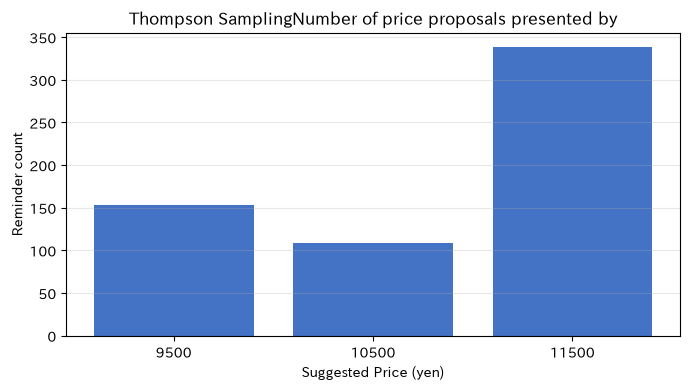
At Thompson Sampling, the order probability for each price proposal is set at $\theta_k\sim\mathrm{Beta}(a_k,b_k)$, and the product of the order probability sampled from the posterior distribution and the gross profit at the time of order is the largest proposal. Limit yourself to comparable projects where price fairness and contract terms are the same.

Check with Python

prices = np.array([9_500, 10_500, 11_500])
cost = 6_200
true_conv = np.array([.46, .39, .30])
a = np.ones(3); b = np.ones(3); counts = np.zeros(3, dtype=int); rewards = np.zeros(3)
for _ in range(600):
    sampled_value = rng.beta(a, b) * (prices - cost)
    arm = int(np.argmax(sampled_value))
    won = rng.random() < true_conv[arm]
    a[arm] += won; b[arm] += 1-won; counts[arm] += 1; rewards[arm] += won * (prices[arm]-cost)
bandit = pd.DataFrame({"price": prices, "trials": counts, "posterior_conversion": a/(a+b), "gross_profit": rewards})
display(bandit)

fig, ax = plt.subplots(figsize=(7, 4))
ax.bar(bandit.price.astype(str), bandit.trials, color="#4472C4")
ax.set_title("Thompson SamplingNumber of price proposals presented by")
ax.set_xlabel("Suggested Price (yen)"); ax.set_ylabel("Reminder count")
ax.grid(axis="y", alpha=.3); plt.tight_layout(); plt.show()

	price	trials	posterior_conversion	gross_profit
0	9500	153	0.47	237,600.00
1	10500	109	0.40	184,900.00
2	11500	338	0.31	545,900.00

Reading the results

The algorithm considers not only the order rate but also the gross profit margin at the time of order, allocating to prices with higher expected profits. On the other hand, if the difficulty of the deal is skewed by price proposal, it can distort learning, so contextual bandits or exclusion rules that condition customer attributes are necessary.

No.058: Bayesian Optimization

Meaning in Practice

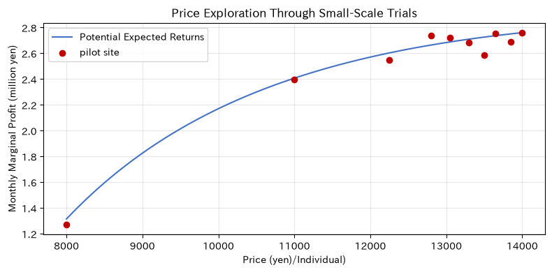
If price verification takes time and you can try it too often, a one-time sale is difficult. Bayesian optimization estimates unobserved points from observed prices and profits, searching for promising prices with fewer attempts.

Approach to Analysis and Modeling

Here, we simplify the Gaussian process concept, creating uncertainty based on average profit and distance in RBF kernel regression. Explore the acquisition function as $\mathrm{UCB}(p)=\mu(p)+\kappa\sigma(p)$. This is a simple implementation for teaching materials, and in the actual test, we will use noisy GP and constrained acquisition functions.

Check with Python

grid = np.linspace(8_000, 14_000, 121)
def objective(p):
    q = 620 * (p / 10_000) ** -1.55
    return (p - 6_500) * q + rng.normal(0, 55_000)

observed_x = [8_000., 11_000., 14_000.]
observed_y = [objective(x) for x in observed_x]
for _ in range(7):
    dist = (grid[:, None] - np.array(observed_x)[None, :]) / 900
    w = np.exp(-0.5 * dist**2) + 1e-9
    mean = (w @ np.array(observed_y)) / w.sum(axis=1)
    nearest = np.min(np.abs(grid[:, None] - np.array(observed_x)[None, :]), axis=1)
    uncertainty = 80_000 * (1 - np.exp(-nearest / 700))
    next_x = grid[np.argmax(mean + 1.4 * uncertainty)]
    observed_x.append(float(next_x)); observed_y.append(objective(next_x))
bo = pd.DataFrame({"price": observed_x, "observed_profit": observed_y})
display(bo.round(0))

true_curve = (grid - 6_500) * 620 * (grid / 10_000) ** -1.55
fig, ax = plt.subplots(figsize=(8, 4))
ax.plot(grid, true_curve/1e6, label="Potential Expected Returns", color="#4472C4")
ax.scatter(bo.price, bo.observed_profit/1e6, color="#C00000", label="pilot site", zorder=3)
ax.set_title("Price Exploration Through Small-Scale Trials")
ax.set_xlabel("Price (yen)/Individual)"); ax.set_ylabel("Monthly Marginal Profit (million yen)")
ax.grid(alpha=.3); ax.legend(); plt.tight_layout(); plt.show()

	price	observed_profit
0	8,000.00	1,271,091.00
1	11,000.00	2,397,138.00
2	14,000.00	2,760,474.00
3	13,300.00	2,685,233.00
4	13,650.00	2,755,292.00
5	12,800.00	2,738,434.00
6	13,850.00	2,691,381.00
7	13,050.00	2,720,481.00
8	13,500.00	2,587,793.00
9	12,250.00	2,549,503.00

Reading the results

From the initial point, attempts are tested in uncertain areas, gradually concentrating toward higher-profit price ranges. Since fewer trial points are influenced by model assumptions, price upper and lower limits, minimum order rates, and customer protection are defined as constraints in advance.

No.059: Reinforcement Learning

Meaning in Practice

If current prices affect future inventory, customer relationships, and learning, single-month optimization is insufficient. Reinforcement learning learns strategies that include future rewards, choosing actions based on the state.

Approach to Analysis and Modeling

Status is the inventory level, behavior is price, and rewards are the sum of marginal profit and storage/out-of-stock penalties. Q Learning

$Q(s,a)\leftarrow Q(s,a)+\alpha[r+\gamma\max_{a'}Q(s',a')-Q(s,a)]$

will be updated. When the demand model is clear, dynamic programming and simulation optimization are first compared.

Check with Python

inventory_levels = np.arange(0, 701, 100)
rl_prices = np.array([9_000, 10_500, 12_000])
Q = np.zeros((len(inventory_levels), len(rl_prices)))
alpha, gamma, epsilon = .12, .92, .15
for episode in range(5000):
    inv = 500
    for t in range(6):
        s = int(np.argmin(abs(inventory_levels-inv)))
        arm = rng.integers(3) if rng.random() < epsilon else int(np.argmax(Q[s]))
        p = rl_prices[arm]
        demand = max(0, int(rng.normal(110*(p/10_000)**-1.6, 12)))
        sold = min(inv, demand); next_inv = min(700, inv-sold+100)
        reward = (p-6_200)*sold - 250*next_inv - 1_500*max(demand-inv, 0)
        ns = int(np.argmin(abs(inventory_levels-next_inv)))
        Q[s, arm] += alpha*(reward + gamma*Q[ns].max()-Q[s, arm])
        inv = next_inv
policy = pd.DataFrame({"inventory": inventory_levels, "recommended_price": rl_prices[np.argmax(Q, axis=1)]})
display(policy)

fig, ax = plt.subplots(figsize=(7, 4))
ax.step(policy.inventory, policy.recommended_price, where="mid", color="#7030A0")
ax.set_title("Recommended pricing strategies by learned inventory level")
ax.set_xlabel("Beginning inventory (units)"); ax.set_ylabel("Suggested Price (Yen)/Individual)")
ax.grid(alpha=.3); plt.tight_layout(); plt.show()

	inventory	recommended_price
0	0	9000
1	100	9000
2	200	9000
3	300	9000
4	400	12000
5	500	12000
6	600	10500
7	700	9000

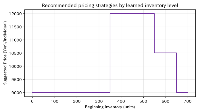
Reading the results

When inventory is low, the basic strategy is to suppress shortages with high prices, and when inventory is high, lower prices to reduce congestion. The details of the table depend on the simulation settings. Before going live, offline evaluation, comparison with conservative measures, price upper and lower limits, and human approval are essential.

No.060: Practical Application

Meaning in Practice

Price optimization alone is not a fixed solution for price optimization with excellent algorithms. Cost mastering, contract terms, sales exceptions, capability planning, approval responsibilities, and effectiveness verification are integrated into a single operation.

Approach to Analysis and Modeling

In practice, we separate the group who set the suggested price and the group who verify based on operational constraints. It stores differences between recommended and adopted values, exception reasons, and track records, monitoring not only profits but also order rates, retention rates, supply compliance, and fairness. Start with decision support and gradually expand the scope of automation.

Check with Python

recommendations = pd.DataFrame({
    "customer": ["AIndustry", "BWorkshop", "Cchemistry", "DPrecision machinery", "EMaterial"],
    "segment": ["large mouth", "backbone", "small mouth", "backbone", "large mouth"],
    "model_price": [11_800, 11_200, 10_100, 11_500, 12_100],
    "contract_floor": [10_800, 10_500, 9_800, 10_700, 11_000],
    "contract_ceiling": [11_500, 11_400, 10_600, 11_300, 11_900],
    "capacity_risk": ["high", "low", "low", "middle", "high"],
})
recommendations["guardrailed_price"] = recommendations.model_price.clip(
    lower=recommendations.contract_floor, upper=recommendations.contract_ceiling)
recommendations["needs_approval"] = (recommendations.model_price != recommendations.guardrailed_price) | recommendations.capacity_risk.eq("high")
display(recommendations)

kpi = pd.DataFrame({
    "KPI": ["marginal interest/Ability time", "Order rate", "Recommended Adoption Rate", "price exception rate", "90Daily Retention Rate"],
    "surveillance video": ["weekly", "weekly", "monthly", "monthly", "quarter"],
    "main person in charge": ["Accounting and Production", "Sales", "Sales Planning", "Sales Planning", "Sales"],
})
display(kpi)

	customer	segment	model_price	contract_floor	contract_ceiling	capacity_risk	guardrailed_price	needs_approval
0	AIndustry	large mouth	11800	10800	11500	high	11500	True
1	BWorkshop	backbone	11200	10500	11400	low	11200	False
2	Cchemistry	small mouth	10100	9800	10600	low	10100	False
3	DPrecision machinery	backbone	11500	10700	11300	middle	11300	True
4	EMaterial	large mouth	12100	11000	11900	high	11900	True

	KPI	surveillance video	main person in charge
0	marginal interest/Ability time	weekly	Accounting and Production
1	Order rate	weekly	Sales
2	Recommended Adoption Rate	monthly	Sales Planning
3	price exception rate	monthly	Sales Planning
4	90Daily Retention Rate	quarter	Sales

Reading the results

Model prices are adjusted at the upper and lower limits of the contract, and projects with high capability risk or those subject to adjustments are subject to approval. By starting from a model that “the model gathers the basis and people control the exception,” rather than “the model decides,” auditability and on-site acceptance can be achieved.

Practical Implications Seen Through Target Exercise

1. It is necessary to connect price reaction estimations, customer value, cost, and capability to the same profit indicator.
2. Static optimization is based on base pricing, Bandit and Bayesian optimization require limited learning, and reinforcement learning requires multi-period problems; this is important.
3. Practical value lies in price ranges and guardrail designs that can withstand estimation errors rather than optimal values.
4. Price is a promise to customers. Explainability, fairness, and contract compliance are treated alongside objective functions.

What is necessary for practical implementation

• Data: Quotation presentation, order receipt and cancellation, quantity, cost, customer attributes, contract, delivery date, and capability are connected by case ID.
• verification: Create a price experiment with a limited target and a preliminary evaluation plan for incremental profit and retention rate
• Business Design: Define upper and lower limits, change frequency, exemptions, approvers, and customer descriptions
• System: Save recommended values, adoption values, reasons for overwriting, and achievements as a history
• surveillance: Regularly monitor demand drift, profits, lost orders, unfair practices between segments, and complaints

Conclusion

Price optimization is not just a calculation of price increases. It is a decision-making system that measures demand, designs customer value, converts profits including supply constraints, and continues to learn safely. As a first step, it is practical to introduce static profit curves and price guardrails into sales meetings targeting one major product and one region.

Consultations for Corporations

At Suri Kobo, we support companies tailored to their data maturity, from estimating price elasticity, designing price and promotional experiments, optimizing profits, implementing them into sales processes, to training for personnel. You can consult with us from the stage of what can be verified with existing data.

📩 Contact Us: surikobo.co.jp/contact Please feel free to consult us first.