A decision-making platform connecting sales, production, and management: 10 Exercises on Manufacturing Marketing Science Practice

This article uses fictitious data from industrial equipment manufacturers to address How to integrate observation, management decision-making, execution, and learning into a single system. The subjects are No.091 to No.100 (Decision Science, OODA, Scenario Analysis, KPI Design, Management Dashboards, AI and Decision Making, Manufacturing DI, Learning from Palantir, Surikoubo’s Vision, Marketing Science in the AI Era).

Not only analytical accuracy but also concretizing “who decides what, when, and what” and “under what conditions should the decision be changed.”

[!NOTE] This material is a notebook previously used by Surikoubo (or personally by the representative, Kazuyama), and has been reconstructed, edited, and published with the company’s permission. All data listed is fictional and has no relation whatsoever to real companies, factories, or figures.

Introduction: Practical Challenges in Manufacturing Covered in This Article

The fictional ‘Koei Industrial’ is an industrial equipment manufacturer that sells standard, high-efficiency, and custom machines. Inquiries are increasing, but sales focus on orders, factories focus on utilization, management focuses on profit, and different figures are presented at each meeting. The question in this article is: Which projects or markets should we allocate limited production capacity and sales resources to?.

Common situations on site

• The more we pursue sales targets, the more unprofitable express projects increase, worsening overtime and delivery delays.
• CRM, quoting, ordering, production, and quality data are fragmented, making it impossible to consistently view the same customer.
• Only the forecast value is presented, and assumptions, uncertainties, and withdrawal conditions are not shared.
• AI proposals end as “reference information” without a responsible person or approval conditions

Why is this issue so difficult to judge?

Sales, gross profit, delivery times, and quality influence each other, and the timing when the effectiveness of these measures becomes apparent also differs. Furthermore, the order probability and material costs are not finalized. Therefore, decisions that clearly state objectives, constraints, and uncertainties are necessary, rather than maximizing a single KPI.

Overview of Exercise covered this time

No.	Theme	Questions answered at management meetings
091	What is Decision Science?	How to compare expected profits and risks
092	OODA	What signs to look for, and when to change course
093	scenario analysis	Can plans endure with pessimism, standards, and optimism?
094	KPI Design	What are the leading indicators that drive the outcome indicators?
095	Management Dashboard	In what order should exceptions be checked?
096	AI and Decision-Making	Under what conditions should AI proposals be adopted?
097	Manufacturing DI	Can changes on the ground be detected early using synthetic indicators?
098	What we can learn from Palantir	How to connect data to business objects for judgment
099	Suri Kobo’s Vision	How to design from PoC to operational implementation
100	Marketing Science in the AI Era	How to build a human-AI learning loop

Preparing the Python environment

It does not rely on external data and uses only numpy, pandas, and matplotlib. Fix the random number seed so you can reproduce the same result. Labels in the graph are displayed in English to avoid differences in Japanese fonts in the running environment.

import sys
import numpy as np
import pandas as pd
import matplotlib
import matplotlib.pyplot as plt
from IPython.display import display

SEED = 42
rng = np.random.default_rng(SEED)
pd.set_option("display.max_columns", 20)
pd.set_option("display.float_format", lambda x: f"{x:,.2f}")
plt.rcParams["figure.figsize"] = (8, 4.5)
plt.rcParams["axes.unicode_minus"] = False

print("Python     :", sys.version.split()[0])
print("numpy      :", np.__version__)
print("pandas     :", pd.__version__)
print("matplotlib :", matplotlib.__version__)
print("random seed:", SEED)

Python     : 3.13.1
numpy      : 2.5.1
pandas     : 3.0.3
matplotlib : 3.11.0
random seed: 42

Creation of Fictional Data

Generates 24-month, 3-product, and 3-region project, order, and operational data. The amount is measured in million yen. orders is generated from the number of projects and order rates, linked to sales, gross profit, on-time delivery rate, and defect rate. This causal structure is an explanatory assumption and is updated in practice through operational knowledge and verification.

months = pd.date_range("2024-01-01", periods=24, freq="MS")
products = ["Standard", "Eco", "Custom"]
regions = ["East", "Central", "West"]
rows = []
for t, month in enumerate(months):
    season = 1 + 0.12 * np.sin(2 * np.pi * t / 12)
    for p in products:
        for r in regions:
            p_mult = {"Standard": 1.0, "Eco": 0.8, "Custom": 0.55}[p]
            r_mult = {"East": 1.15, "Central": 1.0, "West": 0.85}[r]
            leads = max(8, int(rng.poisson(28 * season * p_mult * r_mult * (1 + 0.012*t))))
            quote_days = max(3, rng.normal({"Standard": 7, "Eco": 9, "Custom": 15}[p], 1.8))
            discount = np.clip(rng.normal(0.075 if p != "Custom" else 0.045, 0.018), 0.02, 0.14)
            win_prob = np.clip(0.38 + 0.08*(p == "Eco") - 0.010*quote_days - 0.65*discount + 0.12, 0.12, 0.65)
            orders = rng.binomial(leads, win_prob)
            unit_price = {"Standard": 4.8, "Eco": 6.7, "Custom": 10.5}[p]
            revenue = orders * unit_price * (1-discount)
            utilization = np.clip(rng.normal(0.78 + 0.006*t + 0.05*(p == "Custom"), 0.045), 0.60, 0.98)
            defect_rate = np.clip(0.012 + 0.055*max(utilization-0.82, 0) + rng.normal(0, .002), .004, .04)
            on_time = np.clip(0.98 - 0.55*max(utilization-0.80, 0) - 1.8*defect_rate + rng.normal(0,.01), .78, .99)
            margin_rate = 0.34 - discount - 0.10*(p == "Custom") - 0.35*defect_rate
            rows.append([month,p,r,leads,quote_days,discount,win_prob,orders,revenue,margin_rate,
                         revenue*margin_rate,utilization,defect_rate,on_time])

df = pd.DataFrame(rows, columns=["month","product","region","leads","quote_days","discount",
    "win_prob","orders","revenue","margin_rate","gross_profit","utilization","defect_rate","on_time"])
display(df.head())
print(f"rows={len(df):,}, period={df.month.min():%Y-%m} to {df.month.max():%Y-%m}")

	month	product	region	leads	quote_days	discount	win_prob	orders	revenue	margin_rate	gross_profit	utilization	defect_rate	on_time
0	2024-01-01	Standard	East	37	8.35	0.09	0.36	9	39.23	0.24	9.56	0.72	0.01	0.95
1	2024-01-01	Standard	Central	21	8.58	0.09	0.36	8	34.98	0.25	8.61	0.83	0.01	0.93
2	2024-01-01	Standard	West	25	8.58	0.07	0.37	11	48.89	0.26	12.75	0.75	0.01	0.95
3	2024-01-01	Eco	East	30	9.96	0.08	0.43	10	61.53	0.25	15.55	0.80	0.02	0.95
4	2024-01-01	Eco	Central	20	10.11	0.10	0.42	6	36.37	0.24	8.77	0.74	0.01	0.97

rows=216, period=2024-01 to 2025-12

No.091: What is Decision Science?

Meaning in Practice

Decision science is not just about ‘making predictions.’ Organize options, possible scenarios, the value of outcomes, and constraints, and address them up to Which option to choose. Here, we compare the business and production policies for the next quarter.

Approach to Analysis and Modeling

If we assume the measures $a$, demand $s$, profit $\pi(a,s)$, and state probability $p(s)$, the expected profit is

$E[\pi(a)] = \sum_s p(s)\pi(a,s)$

That’s right. However, since the average alone overlooks the downside, both the standard deviation and the worst value are listed together. Probability is not true; it is an assumption at present.

Check with Python

states = pd.DataFrame({"scenario":["Low","Base","High"], "probability":[0.25,0.50,0.25]})
payoff = pd.DataFrame({
    "Balanced":[46, 61, 72],
    "Growth_priority":[28, 66, 91],
    "Margin_priority":[51, 59, 63]
}, index=states["scenario"])
decision = pd.DataFrame({
    "expected_profit": payoff.mul(states.probability.to_numpy(), axis=0).sum(),
    "risk_std": [np.sqrt(np.average((payoff[c]-np.average(payoff[c],weights=states.probability))**2,
                                    weights=states.probability)) for c in payoff],
    "worst_case": payoff.min()
}).sort_values("expected_profit", ascending=False)
display(payoff)
display(decision.round(1))

	Balanced	Growth_priority	Margin_priority
scenario
Low	46	28	51
Base	61	66	59
High	72	91	63

	expected_profit	risk_std	worst_case
Growth_priority	62.80	22.50	28
Balanced	60.00	9.20	46
Margin_priority	58.00	4.40	51

Reading the results

Growth priority means a large downside even if the expected profit is maximized, while profit priority improves the worst-case value by sacrificing the expected value a bit. At the management meeting, not only should the “maximum expected profit” be decided, but also the minimum profit you want to secure and the conditions under which you will assume additional risks.

No.092：OODA

Meaning in Practice

OODA is a cycle of Observe (observe), Orient (situational judgment), Decide, and Act (execute). Instead of using it as a document preparation procedure for monthly meetings, it is used as an operational design that detects changes and updates decisions.

Approach to Analysis and Modeling

Observe values are compared with reference values, and only exceptions exceeding thresholds are considered for judgment. Here, if the on-time delivery rate is below 92% or the equipment utilization rate exceeds 90%, a simple rule is set to prioritize load adjustment over increased production.

Check with Python

monthly = df.groupby("month").agg(revenue=("revenue","sum"), gross_profit=("gross_profit","sum"),
    utilization=("utilization","mean"), on_time=("on_time","mean"), defect_rate=("defect_rate","mean")).reset_index()
monthly["signal"] = np.select(
    [(monthly.on_time < .92) | (monthly.utilization > .90), monthly.gross_profit.pct_change() < -.08],
    ["Capacity review", "Demand review"], default="Continue")
display(monthly.tail(8).assign(
    utilization=lambda x: x.utilization.map("{:.1%}".format),
    on_time=lambda x: x.on_time.map("{:.1%}".format),
    defect_rate=lambda x: x.defect_rate.map("{:.1%}".format)))

	month	revenue	gross_profit	utilization	on_time	defect_rate	signal
16	2025-05-01	577.78	138.85	86.7%	91.4%	1.5%	Capacity review
17	2025-06-01	545.86	132.93	91.1%	88.9%	1.6%	Capacity review
18	2025-07-01	624.31	140.50	92.9%	87.7%	1.8%	Capacity review
19	2025-08-01	591.95	146.69	89.1%	90.0%	1.6%	Capacity review
20	2025-09-01	628.77	155.17	90.5%	89.1%	1.6%	Capacity review
21	2025-10-01	522.30	122.20	91.4%	88.9%	1.6%	Capacity review
22	2025-11-01	600.21	141.85	92.7%	87.9%	1.8%	Capacity review
23	2025-12-01	522.11	129.40	95.3%	86.5%	1.8%	Capacity review

Reading the results

The speed of OODA is measured not by the number of meetings, but by the number of days from signs to countermeasure implementation. By automatically detecting thresholds and defining the responsible person, deadline, and selectable measures in advance, you can reduce stagnation from observation to execution.

No.093: Scenario Analysis

Meaning in Practice

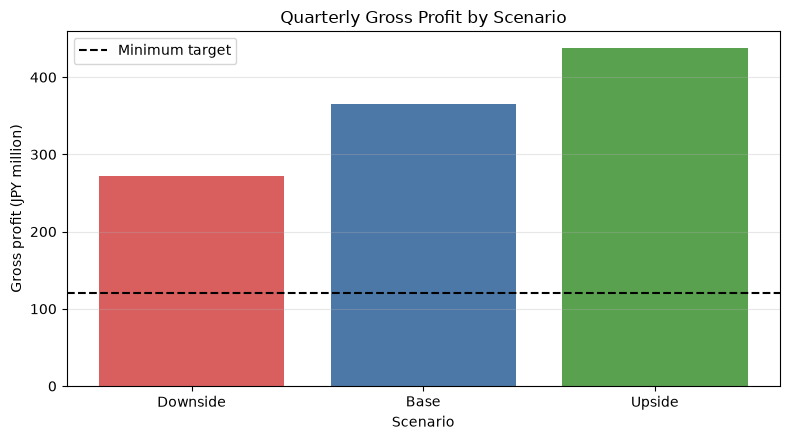
A single budget becomes useless the moment it is removed. Prepare multiple combinations of demand, material costs, and supply capacity to check whether profits and delivery times fall within acceptable ranges in each situation.

Approach to Analysis and Modeling

Simple quarterly gross profit

$G = R_0(1+g)\{m_0-c-0.08\max(u-0.85,0)\}$

Let’s say so. $g$ is the increase in demand, $c$ is the decline in gross profit margin due to rising material costs, and $u$ is the utilization rate. The coefficients in the formula are explanatory assumptions and are estimated in practice from the cost structure.

Check with Python

base_revenue = monthly.revenue.tail(3).sum()
base_margin = monthly.gross_profit.tail(3).sum() / base_revenue
scenarios = pd.DataFrame({
    "scenario":["Downside","Base","Upside"],
    "demand_change":[-.15,0,.18], "material_margin_impact":[.045,.015,.005],
    "utilization":[.80,.88,.96], "probability":[.25,.50,.25]})
scenarios["quarter_revenue"] = base_revenue*(1+scenarios.demand_change)
scenarios["quarter_profit"] = scenarios.quarter_revenue*(base_margin-scenarios.material_margin_impact-
    .08*np.maximum(scenarios.utilization-.85,0))
display(scenarios.round(2))

plt.bar(scenarios.scenario, scenarios.quarter_profit, color=["#d95f5f","#4c78a8","#59a14f"])
plt.axhline(120, color="black", linestyle="--", label="Minimum target")
plt.title("Quarterly Gross Profit by Scenario")
plt.xlabel("Scenario"); plt.ylabel("Gross profit (JPY million)"); plt.grid(axis="y", alpha=.3); plt.legend()
plt.tight_layout(); plt.show()

	scenario	demand_change	material_margin_impact	utilization	probability	quarter_revenue	quarter_profit
0	Downside	-0.15	0.04	0.80	0.25	1,397.93	271.53
1	Base	0.00	0.02	0.88	0.50	1,644.63	364.84
2	Upside	0.18	0.00	0.96	0.25	1,940.66	437.49

Reading the results

If the pessimistic scenario is below the minimum profit, simply lowering the budget is not enough. Mitigation measures that can be implemented in advance, such as renegotiating material prices, selecting projects, and securing outsourcing slots, are linked to activation conditions.

No.094: KPI Design

Meaning in Practice

Sales are important, but by the time results become clear, it often comes too late. We connect the number of orders and estimation speed before receiving orders, and the utilization rate and quality after receiving orders, breaking them down into KPIs that the field can actually drive.

Approach to Analysis and Modeling

Break down sales into “Number of Deals× Order Rate × Average Unit Price,” and connect gross profit to “Sales × Gross Margin.” KPIs need definition, granularity, update frequency, responsible persons, goals, and guardrails.

Check with Python

latest = df[df.month >= df.month.max()-pd.offsets.MonthBegin(2)]
kpi = pd.Series({
    "Leads": latest.leads.sum(),
    "Win rate": latest.orders.sum()/latest.leads.sum(),
    "Avg revenue/order": latest.revenue.sum()/latest.orders.sum(),
    "Gross margin": latest.gross_profit.sum()/latest.revenue.sum(),
    "On-time rate": np.average(latest.on_time, weights=latest.orders),
    "Defect rate": np.average(latest.defect_rate, weights=latest.orders)
}, name="latest_quarter")
targets = pd.Series({"Leads":650,"Win rate":.30,"Avg revenue/order":6.0,"Gross margin":.25,
                     "On-time rate":.94,"Defect rate":.015}, name="target")
kpi_table = pd.concat([kpi, targets], axis=1)
kpi_table["status"] = np.where(
    [kpi[x] <= targets[x] if x=="Defect rate" else kpi[x] >= targets[x] for x in kpi.index], "OK", "Review")
display(kpi_table)

	latest_quarter	target	status
Leads	671.00	650.00	OK
Win rate	0.39	0.30	OK
Avg revenue/order	6.23	6.00	OK
Gross margin	0.24	0.25	Review
On-time rate	0.88	0.94	Review
Defect rate	0.02	0.01	Review

Reading the results

Rather than focusing solely on unsold sales, you can identify the causes of project shortages, declining order rates, and lower unit prices. On the other hand, to prevent discounts that only increase the order rate, we use gross margin and on-time delivery rates as guardrails.

No.095: Management Dashboard

Meaning in Practice

The purpose of dashboards is not to display a lot of information, but to identify exceptions and help those in charge move on to the next action. We design the granularity to be refined into company-wide → products → projects.

Approach to Analysis and Modeling

Compare the latest month’s performance with your goals, and show the differences in color. The three layers of KPI cards, chronology, and breakdown are the minimum structure, and the same definition is used in all meetings.

Check with Python

fig, axes = plt.subplots(2, 2, figsize=(11, 7))
axes[0,0].plot(monthly.month, monthly.revenue, marker="o", ms=3)
axes[0,0].set_title("Monthly Revenue"); axes[0,0].set_xlabel("Month"); axes[0,0].set_ylabel("JPY million"); axes[0,0].grid(alpha=.3)
axes[0,1].plot(monthly.month, monthly.gross_profit, color="#59a14f")
axes[0,1].set_title("Monthly Gross Profit"); axes[0,1].set_xlabel("Month"); axes[0,1].set_ylabel("JPY million"); axes[0,1].grid(alpha=.3)
axes[1,0].plot(monthly.month, monthly.on_time*100, color="#f28e2b")
axes[1,0].axhline(94, color="black", ls="--")
axes[1,0].set_title("On-time Delivery"); axes[1,0].set_xlabel("Month"); axes[1,0].set_ylabel("Percent"); axes[1,0].grid(alpha=.3)
prod = latest.groupby("product").gross_profit.sum().sort_values()
axes[1,1].barh(prod.index, prod.values, color="#4c78a8")
axes[1,1].set_title("Quarterly Profit by Product"); axes[1,1].set_xlabel("JPY million"); axes[1,1].set_ylabel("Product"); axes[1,1].grid(axis="x", alpha=.3)
fig.suptitle("Executive Decision Dashboard", fontsize=14)
plt.tight_layout(); plt.show()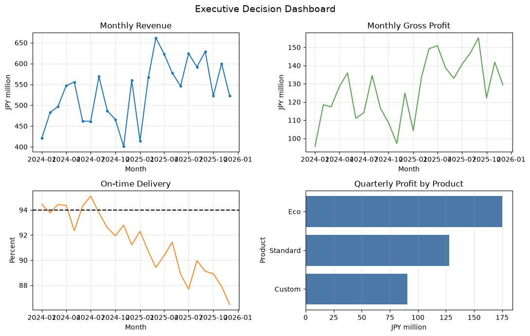

Reading the results

By looking at breakdowns by delivery and product along with changes in profit, you can identify structures such as “selling well but unable to supply” or “small sales but high profitability.” Red lights always include a person responsible, a hypothesis for the cause, and the date for next confirmation.

No.096: AI and Decision-Making

Meaning in Practice

AI can present order probabilities, but adoption decisions—including price, supply constraints, and customer strategies—are handled by humans. You need rules to convert model output to “decision” and exceptions to return to humans.

Approach to Analysis and Modeling

Expected value of $i$ projects

$EV_i = p_i\times GP_i-(1-p_i)C_i$

If the order probability is high $p_i$, expected value is positive, and capacity load is acceptable, priority is given to those with a high order probability. High-value, low-trust deals are not automatically judged but forwarded to human reviews.

Check with Python

opportunities = pd.DataFrame({
    "deal":[f"D-{i:03d}" for i in range(1,9)],
    "ai_win_prob":[.82,.71,.64,.58,.47,.39,.76,.55],
    "gross_profit":[18,11,25,8,20,7,35,13],
    "proposal_cost":[1.5,1.2,3.5,.8,2.7,.7,5.0,1.4],
    "capacity_hours":[120,80,260,70,190,60,340,110],
    "confidence":[.90,.86,.62,.91,.72,.88,.55,.84]})
opportunities["expected_value"] = opportunities.ai_win_prob*opportunities.gross_profit-(1-opportunities.ai_win_prob)*opportunities.proposal_cost
opportunities["decision"] = np.select(
    [(opportunities.confidence < .65) | (opportunities.capacity_hours > 300),
     (opportunities.ai_win_prob >= .55) & (opportunities.expected_value > 5)],
    ["Human review","Prioritize"], default="Nurture")
display(opportunities.sort_values("expected_value", ascending=False))

	deal	ai_win_prob	gross_profit	proposal_cost	capacity_hours	confidence	expected_value	decision
6	D-007	0.76	35	5.00	340	0.55	25.40	Human review
2	D-003	0.64	25	3.50	260	0.62	14.74	Human review
0	D-001	0.82	18	1.50	120	0.90	14.49	Prioritize
4	D-005	0.47	20	2.70	190	0.72	7.97	Nurture
1	D-002	0.71	11	1.20	80	0.86	7.46	Prioritize
7	D-008	0.55	13	1.40	110	0.84	6.52	Prioritize
3	D-004	0.58	8	0.80	70	0.91	4.30	Nurture
5	D-006	0.39	7	0.70	60	0.88	2.30	Nurture

Reading the results

Even with high expected value, large projects with little training data or heavy capacity loads are checked by people. The decision log records AI proposals, adoption or rejection, reasons for overwriting, and results, improving both the model and business rules.

No.097: Manufacturing DI

Meaning in Practice

Here, DI (Decision Intelligence) refers to the concept of connecting data, models, and business knowledge to continuously improve the quality and speed of decision-making. It’s not just about BI or predictive models—it creates a closed-loop process for decisions and outcomes.

Approach to Analysis and Modeling

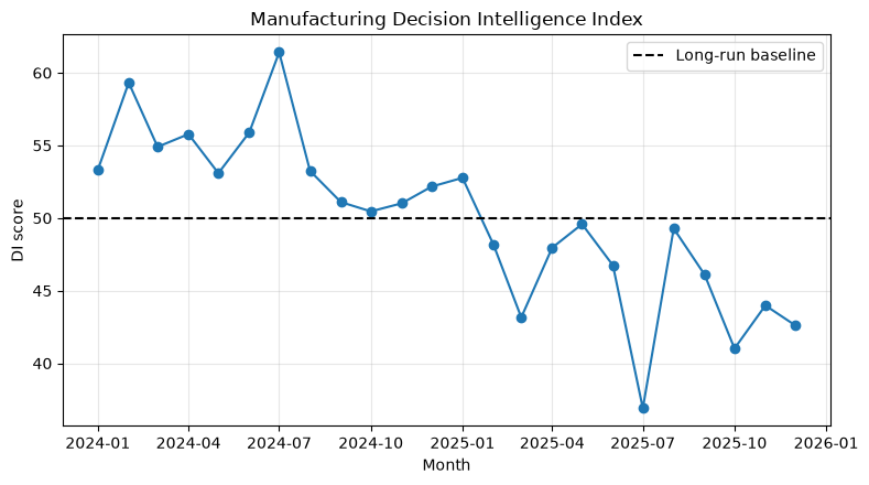
Standardize leading indicators and create synthetic indices where the better the direction of demand, revenue, and supply, the higher the index. Since weights represent management priorities, they are not automatically determined by statistics alone; instead, sensitivity analysis and consensus building are performed.

Check with Python

di = monthly.copy()
di["lead_growth"] = df.groupby("month").leads.sum().pct_change().values
di["margin_rate"] = di.gross_profit/di.revenue
features = pd.DataFrame({
    "demand": di.lead_growth.fillna(0), "margin": di.margin_rate,
    "delivery": di.on_time, "quality": -di.defect_rate, "capacity_buffer": -di.utilization})
z = (features-features.mean())/features.std(ddof=0)
weights = pd.Series({"demand":.20,"margin":.25,"delivery":.25,"quality":.15,"capacity_buffer":.15})
di["DI_score"] = 50 + 10*z.mul(weights).sum(axis=1)
display(di[["month","DI_score","signal"]].tail(8))
plt.plot(di.month, di.DI_score, marker="o")
plt.axhline(50, color="black", ls="--", label="Long-run baseline")
plt.title("Manufacturing Decision Intelligence Index")
plt.xlabel("Month"); plt.ylabel("DI score"); plt.grid(alpha=.3); plt.legend(); plt.tight_layout(); plt.show()

	month	DI_score	signal
16	2025-05-01	49.58	Capacity review
17	2025-06-01	46.74	Capacity review
18	2025-07-01	36.91	Capacity review
19	2025-08-01	49.28	Capacity review
20	2025-09-01	46.10	Capacity review
21	2025-10-01	41.02	Capacity review
22	2025-11-01	43.98	Capacity review
23	2025-12-01	42.61	Capacity review

Reading the results

The composite index provides a clear indication of the direction of the business environment, but there is a risk of hiding the cause. In months when DI declines, we always dig into component indicators to identify whether demand is declining or supply tightening, and adjust countermeasures.

No.098: What to Learn from Palantir

Meaning in Practice

Rather than introducing specific product functions, you will learn a design philosophy that connects data as business objects such as “customers, projects, products, equipment, and orders,” and links analysis results to on-site actions.

Approach to Analysis and Modeling

Define common IDs, relationships, states, permissions, and actionable actions. Rather than just a huge analytical table, it provides a semantic structure showing which projects consume which product capabilities and who approves them.

Check with Python

object_model = pd.DataFrame([
    ["Customer","customer_id","owns","Opportunity","Sales"],
    ["Opportunity","deal_id","requests","Product","Sales"],
    ["Order","order_id","consumes","WorkCenter","Production"],
    ["Product","product_id","uses","Material","Engineering"],
    ["Decision","decision_id","acts_on","Opportunity/Order","Manager"]
], columns=["object","primary_key","relationship","linked_object","owner"])
decision_log = opportunities[["deal","ai_win_prob","expected_value","decision"]].copy()
decision_log["action"] = decision_log.decision.map({"Prioritize":"Assign senior sales", "Nurture":"Schedule follow-up", "Human review":"Convene S&OP review"})
display(object_model)
display(decision_log.head())

	object	primary_key	relationship	linked_object	owner
0	Customer	customer_id	owns	Opportunity	Sales
1	Opportunity	deal_id	requests	Product	Sales
2	Order	order_id	consumes	WorkCenter	Production
3	Product	product_id	uses	Material	Engineering
4	Decision	decision_id	acts_on	Opportunity/Order	Manager

	deal	ai_win_prob	expected_value	decision	action
0	D-001	0.82	14.49	Prioritize	Assign senior sales
1	D-002	0.71	7.46	Prioritize	Assign senior sales
2	D-003	0.64	14.74	Human review	Convene S&OP review
3	D-004	0.58	4.30	Nurture	Schedule follow-up
4	D-005	0.47	7.97	Nurture	Schedule follow-up

Reading the results

The value lies not in data integration itself but in the ability to track actions such as reprioritizing deals and reserving capabilities. Instead of aiming for company-wide integration from the start, we begin with a single important decision and a necessary object.

No.099: Suri Kobo’s Vision

Meaning in Practice

Rather than simply delivering a mathematical model, it is important to advance the definition of management issues, data organization, models, business implementation, and human resource development all in one place. The goal is to achieve a state where the site can improve on its own.

Approach to Analysis and Modeling

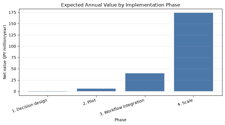
Value is defined as “annual number of judgments × improvement amount per × adoption rate − annual operating costs.” Even if accuracy is high, if it is not adopted, it will not create value. Verify usage and effectiveness through phased implementation.

Check with Python

roadmap = pd.DataFrame({
    "phase":["1. Decision design","2. Pilot","3. Workflow integration","4. Scale"],
    "months":[1,2,3,6], "decisions_per_year":[12,24,60,180],
    "benefit_per_decision":[.8,1.0,1.2,1.3], "adoption_rate":[.25,.50,.72,.85],
    "annual_run_cost":[3,6,12,25]})
roadmap["annual_value"] = roadmap.decisions_per_year*roadmap.benefit_per_decision*roadmap.adoption_rate-roadmap.annual_run_cost
display(roadmap)
plt.bar(roadmap.phase, roadmap.annual_value, color="#4c78a8")
plt.title("Expected Annual Value by Implementation Phase")
plt.xlabel("Phase"); plt.ylabel("Net value (JPY million/year)"); plt.grid(axis="y", alpha=.3)
plt.xticks(rotation=18, ha="right"); plt.tight_layout(); plt.show()

	phase	months	decisions_per_year	benefit_per_decision	adoption_rate	annual_run_cost	annual_value
0	1. Decision design	1	12	0.80	0.25	3	-0.60
1	2. Pilot	2	24	1.00	0.50	6	6.00
2	3. Workflow integration	3	60	1.20	0.72	12	39.84
3	4. Scale	6	180	1.30	0.85	25	173.90

Reading the results

Even if the value is small in the initial stage, the effectiveness expands as the number of decisions and adoption rate increase. The passing criteria for a PoC include not only model accuracy but also utilization rate, decision time, and the recording rate of overwrite reasons.

No.100: Marketing Science in the AI Era

Meaning in Practice

Competitiveness in the AI era is determined not by the performance of individual models, but by the speed at which we connect customer understanding, demand forecasting, supply constraints, and on-site judgment, and learn from the results. AI generates a large number of proposals, and humans are responsible for purpose, constraints, exceptions, and accountability.

Approach to Analysis and Modeling

The value of the initiative is evaluated by subtracting the shadow costs of capacity load and risk penalties from expected gross margin.

$Score_i=p_iGP_i-(1-p_i)C_i-\lambda_h H_i-\lambda_r R_i$

Evaluation metrics are a combination of forecast accuracy, profit, guardrails, adoption rate, and learning speed.

Check with Python

portfolio = opportunities.copy()
portfolio["risk"] = (1-portfolio.confidence)*portfolio.gross_profit
portfolio["decision_score"] = portfolio.expected_value - .012*portfolio.capacity_hours - .35*portfolio.risk
portfolio = portfolio.sort_values("decision_score", ascending=False)
portfolio["cumulative_hours"] = portfolio.capacity_hours.cumsum()
portfolio["selected_under_700h"] = portfolio.cumulative_hours <= 700
display(portfolio[["deal","ai_win_prob","expected_value","capacity_hours","risk","decision_score","selected_under_700h"]])

colors = np.where(portfolio.selected_under_700h, "#59a14f", "#bab0ac")
plt.scatter(portfolio.capacity_hours, portfolio.decision_score, s=portfolio.gross_profit*12, c=colors, alpha=.8)
for _, row in portfolio.iterrows():
    plt.annotate(row.deal, (row.capacity_hours, row.decision_score), xytext=(4,4), textcoords="offset points", fontsize=8)
plt.title("Human-AI Opportunity Portfolio")
plt.xlabel("Required capacity (hours)"); plt.ylabel("Decision score"); plt.grid(alpha=.3); plt.tight_layout(); plt.show()

	deal	ai_win_prob	expected_value	capacity_hours	risk	decision_score	selected_under_700h
6	D-007	0.76	25.40	340	15.75	15.81	True
0	D-001	0.82	14.49	120	1.80	12.42	True
2	D-003	0.64	14.74	260	9.50	8.30	False
1	D-002	0.71	7.46	80	1.54	5.96	False
7	D-008	0.55	6.52	110	2.08	4.47	False
4	D-005	0.47	7.97	190	5.60	3.73	False
3	D-004	0.58	4.30	70	0.72	3.21	False
5	D-006	0.39	2.30	60	0.84	1.29	False

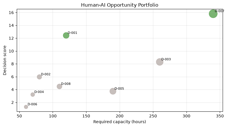
Reading the results

Instead of ranking orders based solely on probability of order, the priorities shift when considering profit, capability, and model reliability. By accumulating the reasons for overwriting and the final result, you can update the next score and judging rules. This is the learning loop between humans and AI.

Practical Implications Seen Through Target Exercise

1. Instead of predictions, use options, constraints, and decision deadlines as the entry point for analysis.
2. Treating sales, profit, delivery dates, and quality within the same decision-making model
3. Decide countermeasures and activation conditions for each scenario in advance
4. Record AI proposals, acceptance or rejection, reasons for overwriting, and results as decision logs
5. Integrating dashboards and actions from the person in charge into a single workflow

What is necessary for practical implementation

• Decision Review: Identify frequency, responsible person, options, deadlines, and current required time
• Data Contracts: Define KPIs, common IDs, update frequency, handling of missing items, and access rights
• Verification Design: In addition to forecasting accuracy, compare profits, delivery times, adoption rates, and decision times before and after implementation.
• Governance: Clearly define the scope of automation, human approval conditions, stopping conditions, and audit logs
• Operational Structure: Appoint a person responsible for model monitoring, KPI review, on-site education, and improvement backlog

Conclusion

From No.091 to No.100, we examined the entire flow from decision science to OODA, scenarios, KPIs, dashboards, AI, DI, business objects, and implementation roadmaps. Marketing science in manufacturing is a management technique that not only analyzes demand but also addresses how to connect customers, projects, and production capacity under supply constraints.

Consultations for Corporations

At Surikoubo, we support everything from management dashboards, demand and order forecasting, prioritization of sales projects, S&OP, and decision-making AI conceptualization to PoC and operational implementation. You can consult with us even when you want to organize which decisions to start with.

📩 Contact Us: surikobo.co.jp/contact Please feel free to consult us first.