
100本ノック / シミュレーション / シミュレーション100本ノック
製造業シミュレーション実践|生産計画・在庫・設備投資をPythonで意思決定
変動に強い工場運営を設計する:製造業シミュレーション実践 No.091〜No.100
需要、設備、人員、在庫、調達は相互に影響します。本 notebook では、架空の精密ポンプ工場を題材に、個別最適の試算を経営・工場運営の一つの意思決定系へつなげます。No.091〜No.100を通じて、計画値だけでなく変動幅、下振れリスク、投資回収、KPIのトレードオフを可視化します。
[!NOTE] 本資料は、数理工房 (もしくは代表である和山個人) が過去に企業研修において使用した notebook を企業様の許可を得て再構成・編集のうえ公開しています。
掲載データはすべて架空のものであり、実在する企業・工場・数値とは一切関係ありません。
はじめに:この記事で扱う製造業の実務課題
月次S&OPでは、販売計画、生産能力、在庫、購買、人員、設備投資を同時に整合させる必要があります。しかし平均需要だけで計画すると、需要の山、故障、納入遅延が重なったときに欠品や残業が急増します。本稿の目的は「未来を一点で当てる」ことではなく、複数の仮定を再現可能な形で比較し、意思決定の頑健性を高めることです。
現場でよくある状況
- 部門ごとに前提とKPIが異なり、同じシナリオを見ていない
- 能力増強案が提示されても、需要変動や立上げロスを含む回収確率が分からない
- 安全在庫、人員、外注の判断が経験則に依存する
- デジタルツインが可視化で止まり、計画変更や承認に接続しない
なぜこの問題は判断が難しいのか
因果関係が循環するためです。増産は在庫を増やしますが、故障や部材不足があれば仕掛品だけが増えます。在庫削減は運転資本を改善しますが、納入遅延への耐性を下げます。したがって、平均値に加えて分位点、制約、費用、サービス水準を同じモデルで比較します。
今回扱うノックの全体像
| No. | テーマ | 主な意思決定 |
|---|---|---|
| 091 | 生産計画 | 需要変動下の月次生産量 |
| 092 | 工場レイアウト | 搬送距離と混雑の削減 |
| 093 | 設備投資 | 能力増強の回収可能性 |
| 094 | 人員配置 | スキル制約下の配員 |
| 095 | 在庫最適化 | 発注点と安全在庫 |
| 096 | サプライチェーン | 調達途絶への耐性 |
| 097 | 需要予測とシミュレーション | 予測誤差を含む計画 |
| 098 | KPI | 利益・納期・在庫の両立 |
| 099 | 製造業デジタルツイン | 観測値による状態更新 |
| 100 | 製造業版Palantirの基盤 | データ・モデル・意思決定の統合 |
Python 環境の準備
NumPyで固定シードの乱数を生成し、pandasで表を扱い、matplotlibで可視化します。外部データ、seaborn、外部APIは使用しません。同じ入力とseedから同じ結果を再現できることは、会議での説明責任やモデル変更管理の前提です。
import sys
import numpy as np
import pandas as pd
import matplotlib
import matplotlib.pyplot as plt
from IPython.display import display

SEED = 20260712
rng = np.random.default_rng(SEED)
pd.set_option("display.float_format", lambda x: f"{x:,.2f}")
print("Python     :", sys.version.split()[0])
print("NumPy      :", np.__version__)
print("pandas     :", pd.__version__)
print("matplotlib :", matplotlib.__version__)
print("random seed:", SEED)
Python : 3.13.1
NumPy : 2.5.1
pandas : 3.0.3
matplotlib : 3.11.0
random seed: 20260712架空データの作成
対象は製品A・B・Cを組立・検査して出荷する工場です。12か月の基準需要、単価、変動係数、工程負荷を作ります。データ生成と業務ルールを分離しておくと、実データへ置き換える際の影響範囲を限定できます。
months = pd.date_range("2026-01-01", periods=12, freq="MS")
products = pd.DataFrame({
    "product": ["A", "B", "C"],
    "unit_price_kJPY": [82, 105, 138],
    "unit_margin_kJPY": [31, 39, 52],
    "demand_cv": [0.12, 0.18, 0.25],
    "assembly_h": [0.80, 1.05, 1.35],
    "inspection_h": [0.25, 0.35, 0.50],
})
base = np.array([420, 280, 160])
season = 1 + 0.12 * np.sin(2 * np.pi * (np.arange(12) - 1) / 12)
demand_plan = pd.DataFrame(
    (season[:, None] * base[None, :]).round().astype(int),
    index=months, columns=products["product"]
)
display(products)
display(demand_plan.head())| product | unit_price_kJPY | unit_margin_kJPY | demand_cv | assembly_h | inspection_h | |
|---|---|---|---|---|---|---|
| 0 | A | 82 | 31 | 0.12 | 0.80 | 0.25 |
| 1 | B | 105 | 39 | 0.18 | 1.05 | 0.35 |
| 2 | C | 138 | 52 | 0.25 | 1.35 | 0.50 |
| product | A | B | C |
|---|---|---|---|
| 2026-01-01 | 395 | 263 | 150 |
| 2026-02-01 | 420 | 280 | 160 |
| 2026-03-01 | 445 | 297 | 170 |
| 2026-04-01 | 464 | 309 | 177 |
| 2026-05-01 | 470 | 314 | 179 |
No.091:生産計画シミュレーション
実務での意味/分析・モデル化の考え方
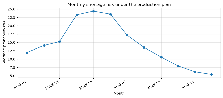
月次計画は需要平均を満たすだけでは不十分です。能力上限と期首在庫を考慮し、欠品と過剰在庫がどの程度の確率で発生するかを確認します。
需要 、生産 、期末在庫 の基本関係は です。在庫が負になる部分を欠品とし、能力制約の下で複数回シミュレーションします。
Pythonで確認する
n_sim = 1000
plan_total = demand_plan.sum(axis=1).to_numpy()
demand_total = rng.normal(plan_total, plan_total * 0.16, size=(n_sim, 12)).clip(0)
capacity = 930
production = np.minimum(capacity, plan_total * 1.04)
inventory = np.zeros((n_sim, 13)); inventory[:, 0] = 120
shortage = np.zeros((n_sim, 12))
for t in range(12):
    available = inventory[:, t] + production[t]
    shortage[:, t] = np.maximum(demand_total[:, t] - available, 0)
    inventory[:, t+1] = np.maximum(available - demand_total[:, t], 0)
result_91 = pd.DataFrame({"month": months, "plan": plan_total, "production": production,
                          "median_ending_inventory": np.median(inventory[:,1:], axis=0),
                          "shortage_probability": (shortage > 0).mean(axis=0)})
display(result_91.round(2))
fig, ax = plt.subplots(figsize=(9, 4)); ax.plot(months, result_91["shortage_probability"]*100, marker="o")
ax.set(title="Monthly shortage risk under the production plan", xlabel="Month", ylabel="Shortage probability (%)")
ax.grid(True, alpha=.3); fig.autofmt_xdate(); plt.tight_layout(); plt.show()
/var/folders/3y/fmw40k0x78xblvb3gkcyvy1h0000gn/T/ipykernel_25456/1898123177.py:15: UserWarning: obj.round has no effect with datetime, timedelta, or period dtypes. Use obj.dt.round(...) instead.
display(result_91.round(2))| month | plan | production | median_ending_inventory | shortage_probability | |
|---|---|---|---|---|---|
| 0 | 2026-01-01 | 808 | 840.32 | 151.74 | 0.12 |
| 1 | 2026-02-01 | 860 | 894.40 | 183.10 | 0.14 |
| 2 | 2026-03-01 | 912 | 930.00 | 206.32 | 0.15 |
| 3 | 2026-04-01 | 950 | 930.00 | 188.65 | 0.23 |
| 4 | 2026-05-01 | 963 | 930.00 | 181.20 | 0.24 |
| 5 | 2026-06-01 | 950 | 930.00 | 180.24 | 0.24 |
| 6 | 2026-07-01 | 912 | 930.00 | 204.88 | 0.17 |
| 7 | 2026-08-01 | 860 | 894.40 | 264.19 | 0.14 |
| 8 | 2026-09-01 | 808 | 840.32 | 319.11 | 0.11 |
| 9 | 2026-10-01 | 770 | 800.80 | 353.34 | 0.08 |
| 10 | 2026-11-01 | 757 | 787.28 | 397.61 | 0.06 |
| 11 | 2026-12-01 | 770 | 800.80 | 439.14 | 0.05 |
結果の読み取り
欠品確率が高い月は、単純な一律増産ではなく、前月の先行生産、残業枠、外注枠を組み合わせる候補です。中央値在庫が積み上がる月と欠品月が併存する場合、年間能力不足よりも月間の能力配分が問題だと読めます。
No.092:工場レイアウトシミュレーション
実務での意味/分析・モデル化の考え方
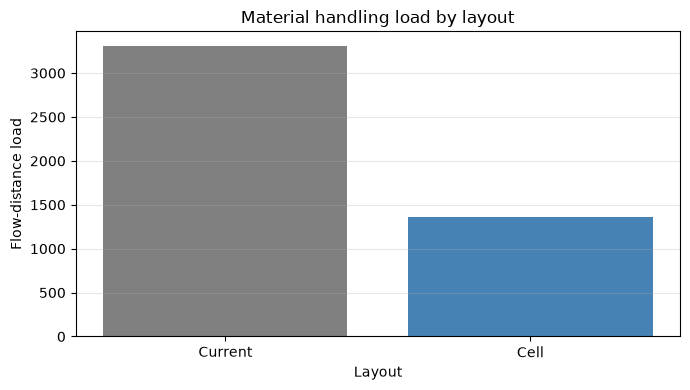
レイアウト変更は搬送距離だけでなく、通路混雑、安全性、移設停止を含む投資判断です。ここでは工程間フローと座標から、現状案とセル化案の搬送負荷を比較します。
工程 間の搬送回数を 、マンハッタン距離を とすると、搬送負荷は です。混雑を表す確率的な待ち時間も加えます。
Pythonで確認する
flows = {("Receiving","Machining"):80, ("Machining","Assembly"):140, ("Assembly","Inspection"):130, ("Inspection","Shipping"):120}
layouts = {"Current":{"Receiving":(0,0),"Machining":(6,1),"Assembly":(2,6),"Inspection":(7,6),"Shipping":(9,1)},
           "Cell":{"Receiving":(0,0),"Machining":(3,1),"Assembly":(5,2),"Inspection":(7,2),"Shipping":(9,1)}}
rows=[]
for name, pos in layouts.items():
    distance_load=sum(f*(abs(pos[a][0]-pos[b][0])+abs(pos[a][1]-pos[b][1])) for (a,b),f in flows.items())
    congestion=rng.lognormal(mean=np.log(distance_load*0.018), sigma=.18, size=1000)
    rows.append([name,distance_load,np.mean(congestion),np.percentile(congestion,95)])
result_92=pd.DataFrame(rows,columns=["layout","distance_load","mean_delay_min","p95_delay_min"])
display(result_92.round(1))
fig, ax=plt.subplots(figsize=(7,4)); ax.bar(result_92["layout"],result_92["distance_load"],color=["gray","steelblue"])
ax.set(title="Material handling load by layout",xlabel="Layout",ylabel="Flow-distance load"); ax.grid(True,axis="y",alpha=.3); plt.tight_layout(); plt.show()| layout | distance_load | mean_delay_min | p95_delay_min | |
|---|---|---|---|---|
| 0 | Current | 3310 | 61.30 | 81.70 |
| 1 | Cell | 1360 | 24.90 | 32.70 |
結果の読み取り
セル化案で搬送負荷と95%点の遅延が下がれば、平均効率だけでなく繁忙時の安定性にも効果があります。実導入では防火区画、保全スペース、フォークリフトと歩行者の交差、移設中の減産を制約に追加します。
No.093:設備投資シミュレーション
実務での意味/分析・モデル化の考え方
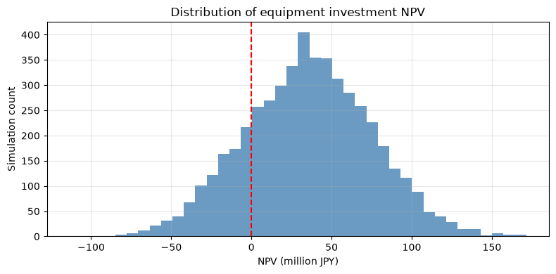
設備投資では、平均NPVが正でも回収できない確率が高ければ意思決定は難しくなります。需要成長、稼働率、立上げ遅れを乱数化して投資案を評価します。
とし、キャッシュフローの不確実性をモンテカルロ法で伝播させます。
Pythonで確認する
n=5000; years=np.arange(1,6); investment=180_000; discount=.08
growth=rng.normal(.045,.035,n); uptime=rng.beta(35,3,n); ramp_delay=rng.choice([0,1,2],n,p=[.65,.25,.10])
npvs=np.full(n,-investment,dtype=float)
for y in years:
    volume=4200*(1+growth)**y*uptime
    volume=np.where(y<=ramp_delay,volume*.55,volume)
    cash=volume*18-22_000
    npvs += cash/(1+discount)**y
result_93=pd.Series({"mean_NPV_kJPY":npvs.mean(),"median_NPV_kJPY":np.median(npvs),"P(NPV>0)":(npvs>0).mean(),"P10_NPV_kJPY":np.percentile(npvs,10)})
display(result_93.to_frame("value").round(2))
fig,ax=plt.subplots(figsize=(8,4)); ax.hist(npvs/1000,bins=40,color="steelblue",alpha=.8); ax.axvline(0,color="red",linestyle="--")
ax.set(title="Distribution of equipment investment NPV",xlabel="NPV (million JPY)",ylabel="Simulation count"); ax.grid(True,alpha=.3); plt.tight_layout(); plt.show()| value | |
|---|---|
| mean_NPV_kJPY | 35,512.67 |
| median_NPV_kJPY | 35,614.25 |
| P(NPV>0) | 0.81 |
| P10_NPV_kJPY | -16,809.36 |
結果の読み取り
採択判断では平均NPVだけでなく、NPV正の確率と下位10%を見ます。下振れが大きい場合は、一括投資を段階投資に変える、需要契約を確保してから発注する、立上げ支援を契約条件に入れる、といったリスク低減策を比較します。
No.094:人員配置シミュレーション
実務での意味/分析・モデル化の考え方
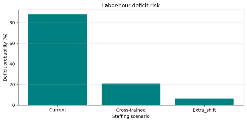
人数が足りていても、必要スキルが一致しなければラインは動きません。組立・検査の技能保有率、欠勤、応援可能性を含む配員を比較します。
必要工数と供給工数の差を不足工数とし、欠勤をベルヌーイ試行で再現します。多能工化は人数増ではなくスキル代替性を上げる施策として評価します。
Pythonで確認する
scenarios={"Current":(.08,.55),"Cross-trained":(.08,.80),"Extra_shift":(.05,.85)}
rows=[]
for name,(absence,qualified) in scenarios.items():
    present=rng.binomial(24,1-absence,2000)
    skilled=rng.binomial(present,qualified)
    supplied=skilled*7.2
    required=rng.normal(112,12,2000)
    deficit=np.maximum(required-supplied,0)
    rows.append([name,deficit.mean(),np.percentile(deficit,95),(deficit>0).mean()])
result_94=pd.DataFrame(rows,columns=["scenario","mean_deficit_h","p95_deficit_h","deficit_probability"])
display(result_94.round(2))
fig,ax=plt.subplots(figsize=(8,4)); ax.bar(result_94["scenario"],result_94["deficit_probability"]*100,color="teal")
ax.set(title="Labor-hour deficit risk",xlabel="Staffing scenario",ylabel="Deficit probability (%)"); ax.grid(True,axis="y",alpha=.3); plt.tight_layout(); plt.show()| scenario | mean_deficit_h | p95_deficit_h | deficit_probability | |
|---|---|---|---|---|
| 0 | Current | 25.51 | 59.40 | 0.88 |
| 1 | Cross-trained | 2.46 | 17.72 | 0.21 |
| 2 | Extra_shift | 0.66 | 2.82 | 0.06 |
結果の読み取り
多能工化で不足確率が大きく下がるなら、恒常的な増員より教育投資が効く可能性があります。ただし技能を二値で扱うのは簡略化です。実務では資格、有効期限、習熟度、指導者、連続勤務、本人希望を制約として管理します。
No.095:在庫最適化シミュレーション
実務での意味/分析・モデル化の考え方
安全在庫は欠品を防ぐ一方、保管費と陳腐化リスクを増やします。発注点候補をシミュレーションし、サービス水準と総費用を比較します。
発注点は概ね です。ただしリードタイム変動やロット制約があるため、日次の在庫推移を直接再現します。
Pythonで確認する
def inventory_policy(rop, days=365, reps=300):
    costs=[]; fill=[]
    for _ in range(reps):
        inv=rop+180; on_order=[]; demand_total=served=holding=orders=0
        for day in range(days):
            inv += sum(q for due,q in on_order if due==day); on_order=[x for x in on_order if x[0]>day]
            d=max(0,int(rng.normal(28,7))); demand_total+=d; s=min(inv,d); served+=s; inv-=s; holding+=inv
            if inv+sum(q for _,q in on_order)<=rop:
                on_order.append((day+int(rng.integers(4,9)),180)); orders+=1
        costs.append(holding*.12+orders*4_000+(demand_total-served)*1_800); fill.append(served/demand_total)
    return np.mean(costs),np.mean(fill)
result_95=pd.DataFrame([(r,*inventory_policy(r)) for r in range(100,301,25)],columns=["reorder_point","annual_cost_kJPY","fill_rate"])
display(result_95.round(3))
fig,ax1=plt.subplots(figsize=(8,4)); ax1.plot(result_95["reorder_point"],result_95["annual_cost_kJPY"],marker="o",label="Cost")
ax1.set(title="Inventory policy trade-off",xlabel="Reorder point (units)",ylabel="Annual cost (kJPY)"); ax1.grid(True,alpha=.3)
ax2=ax1.twinx(); ax2.plot(result_95["reorder_point"],result_95["fill_rate"]*100,color="darkorange",marker="s",label="Fill rate"); ax2.set_ylabel("Fill rate (%)"); plt.tight_layout(); plt.show()| reorder_point | annual_cost_kJPY | fill_rate | |
|---|---|---|---|
| 0 | 100 | 4,205,229.20 | 0.78 |
| 1 | 125 | 2,972,266.99 | 0.85 |
| 2 | 150 | 1,902,245.51 | 0.91 |
| 3 | 175 | 1,099,789.77 | 0.95 |
| 4 | 200 | 453,631.91 | 0.99 |
| 5 | 225 | 269,555.54 | 1.00 |
| 6 | 250 | 231,186.30 | 1.00 |
| 7 | 275 | 230,062.74 | 1.00 |
| 8 | 300 | 231,307.18 | 1.00 |
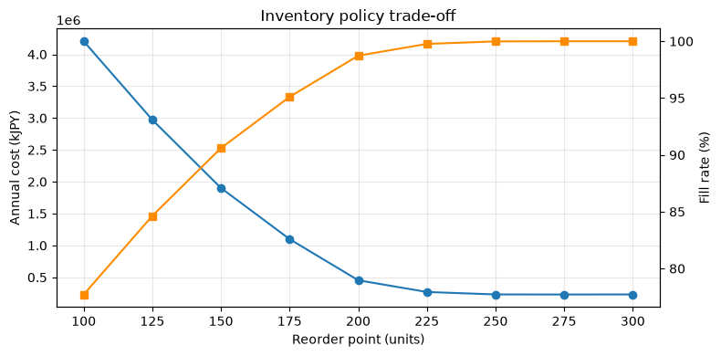
結果の読み取り
最低サービス水準を満たす候補の中から総費用が小さい発注点を選ぶのが基本です。重要顧客向け部品と汎用品で欠品損失は異なるため、全品一律の在庫日数ではなく、品目別のサービス水準を合意する必要があります。
No.096:サプライチェーンシミュレーション
実務での意味/分析・モデル化の考え方
単価の安い単一調達は、途絶時の損失を含めると必ずしも安くありません。単一調達、二社購買、緊急調達の年間総費用と停止日数を比較します。
期待調達費に、遅延・途絶による操業停止費を加えます。相関した災害リスクや同一地域依存を見落とさないことが重要です。
Pythonで確認する
policies={"Single source":(1.00,.08,0),"Dual source":(1.06,.025,0),"Dual + emergency":(1.10,.012,6000)}
rows=[]
for name,(price_factor,disrupt_p,emergency) in policies.items():
    costs=[]; stops=[]
    for _ in range(3000):
        disrupted=rng.random(12)<disrupt_p; stop_days=(rng.integers(2,12,12)*disrupted).sum()
        procurement=12*15_000*price_factor; total=procurement+stop_days*9_000+emergency*(stop_days>0)
        costs.append(total); stops.append(stop_days)
    rows.append([name,np.mean(costs),np.percentile(costs,95),np.mean(stops),(np.array(stops)>0).mean()])
result_96=pd.DataFrame(rows,columns=["policy","mean_cost_kJPY","p95_cost_kJPY","mean_stop_days","disruption_probability"])
display(result_96.round(2))
fig,ax=plt.subplots(figsize=(8,4)); ax.bar(result_96["policy"],result_96["p95_cost_kJPY"]/1000,color="slateblue")
ax.set(title="Supply policy downside cost",xlabel="Sourcing policy",ylabel="95th percentile cost (million JPY)"); ax.grid(True,axis="y",alpha=.3); plt.tight_layout(); plt.show()| policy | mean_cost_kJPY | p95_cost_kJPY | mean_stop_days | disruption_probability | |
|---|---|---|---|---|---|
| 0 | Single source | 235,824.00 | 360,000.00 | 6.20 | 0.61 |
| 1 | Dual source | 207,753.00 | 289,800.00 | 1.88 | 0.25 |
| 2 | Dual + emergency | 207,448.00 | 276,000.00 | 0.96 | 0.14 |
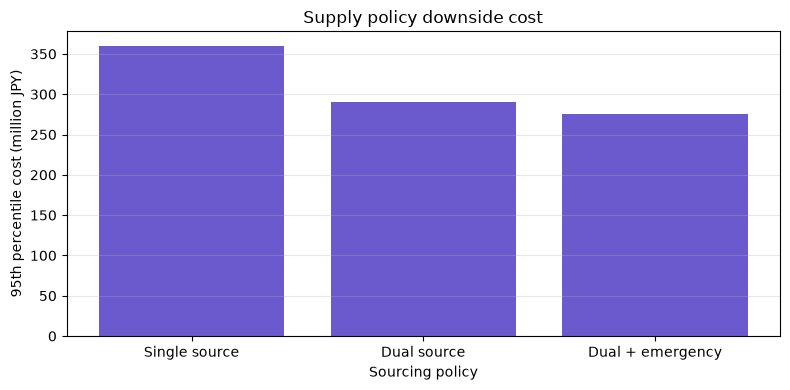
結果の読み取り
二社購買は平時単価を上げても、95%点の総費用と停止日数を下げる可能性があります。BCP判断では期待費用だけでなく、最大許容停止日数、代替材の認定期間、金型・治具の所在、サプライヤーの二次調達先まで確認します。
No.097:需要予測とシミュレーション
実務での意味/分析・モデル化の考え方
予測値をそのまま生産計画に置くと、予測誤差を無視します。点予測と誤差分布を分離し、上方バイアス・下方バイアスを含む計画バッファを比較します。
実績を 、予測を とし、誤差 を再標本化します。MAEだけでなく、誤差を計画へ伝播させた欠品費と在庫費で判断します。
Pythonで確認する
history_actual=700+35*np.sin(np.arange(36)*2*np.pi/12)+rng.normal(0,55,36)
history_forecast=700+35*np.sin(np.arange(36)*2*np.pi/12)
errors=history_actual-history_forecast
future_forecast=700+35*np.sin(np.arange(36,48)*2*np.pi/12)
buffers=[0,.5,1.0,1.5]; rows=[]
for z in buffers:
    plan=future_forecast+z*errors.std()
    simulated=future_forecast+rng.choice(errors,size=(3000,12),replace=True)
    shortage=np.maximum(simulated-plan,0).sum(axis=1); excess=np.maximum(plan-simulated,0).sum(axis=1)
    cost=shortage*2.4+excess*.35
    rows.append([z,cost.mean(),(shortage==0).mean(),shortage.mean(),excess.mean()])
result_97=pd.DataFrame(rows,columns=["buffer_sigma","mean_cost_kJPY","no_shortage_probability","mean_shortage","mean_excess"])
display(result_97.round(2))
fig,ax=plt.subplots(figsize=(8,4)); ax.plot(result_97["buffer_sigma"],result_97["mean_cost_kJPY"],marker="o")
ax.set(title="Planning buffer versus expected cost",xlabel="Buffer (forecast error sigma)",ylabel="Expected cost (kJPY)"); ax.grid(True,alpha=.3); plt.tight_layout(); plt.show()| buffer_sigma | mean_cost_kJPY | no_shortage_probability | mean_shortage | mean_excess | |
|---|---|---|---|---|---|
| 0 | 0.00 | 563.81 | 0.01 | 193.48 | 284.18 |
| 1 | 0.50 | 404.55 | 0.01 | 99.52 | 473.42 |
| 2 | 1.00 | 329.96 | 0.16 | 35.26 | 700.96 |
| 3 | 1.50 | 341.27 | 0.51 | 1.58 | 964.23 |
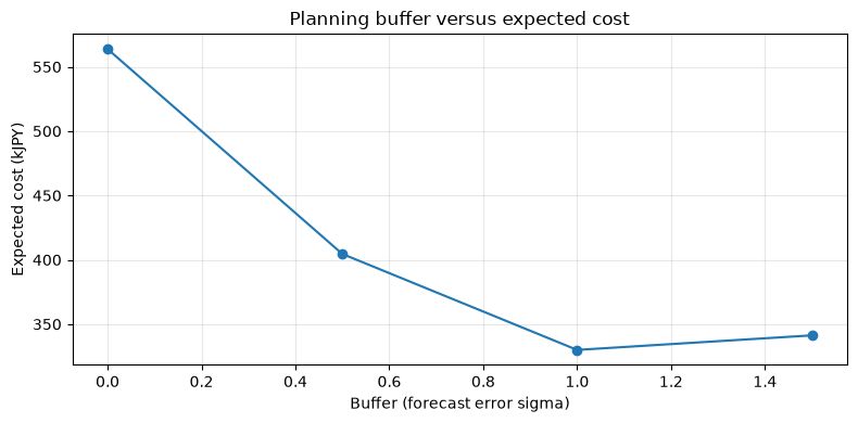
結果の読み取り
予測精度が同じでも、欠品費と在庫費の比で適切なバッファは変わります。また予測誤差に偏りがあれば、バッファ追加より先に予測プロセスを修正します。販促、失注、受注残など観測の意味を統一することも不可欠です。
No.098:KPIシミュレーション
実務での意味/分析・モデル化の考え方
単一KPIの最大化は副作用を生みます。高い稼働率は仕掛品と納期を悪化させることがあり、在庫削減は欠品を増やします。運転方針ごとのKPIを同じシナリオで比較します。
利益、OTIF(納期・数量遵守率)、在庫回転、残業を正規化してスコア化します。ただし重みは経営判断であり、モデルが自動的に決めるものではありません。
Pythonで確認する
policies=[("Lean",.96,.92,10.2,140), ("Balanced",.985,.97,8.4,210), ("Service first",.995,.985,6.3,330)]
rows=[]
for name,yield_rate,otif,turns,overtime in policies:
    profit=420_000*yield_rate + 95_000*otif + rng.normal(0,8000,1500)-overtime*55
    rows.append([name,profit.mean(),otif,turns,overtime])
result_98=pd.DataFrame(rows,columns=["policy","expected_profit_kJPY","OTIF","inventory_turns","overtime_h"])
for c in ["expected_profit_kJPY","OTIF","inventory_turns"]:
    result_98[c+"_score"]=(result_98[c]-result_98[c].min())/(result_98[c].max()-result_98[c].min())
result_98["overtime_score"]=1-(result_98["overtime_h"]-result_98["overtime_h"].min())/(result_98["overtime_h"].max()-result_98["overtime_h"].min())
result_98["balanced_score"]=result_98[["expected_profit_kJPY_score","OTIF_score","inventory_turns_score","overtime_score"]].mean(axis=1)
display(result_98[["policy","expected_profit_kJPY","OTIF","inventory_turns","overtime_h","balanced_score"]].round(3))
fig,ax=plt.subplots(figsize=(8,4)); ax.bar(result_98["policy"],result_98["balanced_score"],color="seagreen")
ax.set(title="Multi-KPI policy score",xlabel="Operating policy",ylabel="Balanced score"); ax.grid(True,axis="y",alpha=.3); plt.tight_layout(); plt.show()| policy | expected_profit_kJPY | OTIF | inventory_turns | overtime_h | balanced_score | |
|---|---|---|---|---|---|---|
| 0 | Lean | 483,023.36 | 0.92 | 10.20 | 140 | 0.50 |
| 1 | Balanced | 494,383.01 | 0.97 | 8.40 | 210 | 0.73 |
| 2 | Service first | 493,255.15 | 0.98 | 6.30 | 330 | 0.47 |
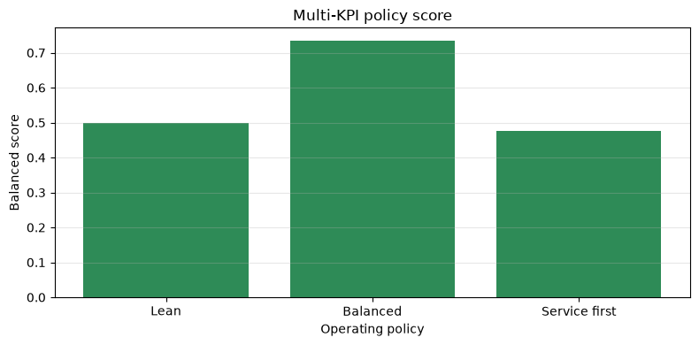
結果の読み取り
バランス案が総合点で優位でも、OTIFの最低基準を下回る案は失格にすべきです。重み付き平均は説明用の補助であり、法令、安全、品質保証、顧客契約の制約を相殺してはいけません。感度分析と経営会議での重み合意が必要です。
No.099:製造業デジタルツイン構築
実務での意味/分析・モデル化の考え方
デジタルツインは3D表示ではなく、現実の観測でモデル状態を更新し、将来を予測して行動へつなぐ仕組みです。ここでは設備の劣化状態をセンサー値で逐次補正します。
予測状態を 、観測を とすると、更新は です。簡易な一次元カルマンフィルタで、観測ノイズをならしながら劣化を追跡します。
Pythonで確認する
days=np.arange(60); true_health=100-.32*days+np.cumsum(rng.normal(0,.18,60)); sensor=true_health+rng.normal(0,2.2,60)
estimate=[]; x=100.; p=4.; q=.25; r=2.2**2
for y in sensor:
    x_pred=x-.32; p_pred=p+q; k=p_pred/(p_pred+r); x=x_pred+k*(y-x_pred); p=(1-k)*p_pred; estimate.append(x)
result_99=pd.DataFrame({"day":days,"sensor":sensor,"estimated_health":estimate,"true_health_for_validation":true_health})
display(result_99.tail().round(2))
fig,ax=plt.subplots(figsize=(9,4)); ax.plot(days,sensor,".",alpha=.45,label="Sensor"); ax.plot(days,estimate,label="Twin estimate",linewidth=2); ax.plot(days,true_health,"--",label="Validation truth")
ax.axhline(82,color="red",linestyle=":",label="Maintenance threshold"); ax.set(title="Digital twin state update",xlabel="Day",ylabel="Health index"); ax.grid(True,alpha=.3); ax.legend(); plt.tight_layout(); plt.show()| day | sensor | estimated_health | true_health_for_validation | |
|---|---|---|---|---|
| 55 | 55 | 87.34 | 86.10 | 85.41 |
| 56 | 56 | 83.99 | 85.41 | 85.25 |
| 57 | 57 | 85.49 | 85.17 | 84.97 |
| 58 | 58 | 83.38 | 84.55 | 84.56 |
| 59 | 59 | 84.04 | 84.19 | 84.26 |
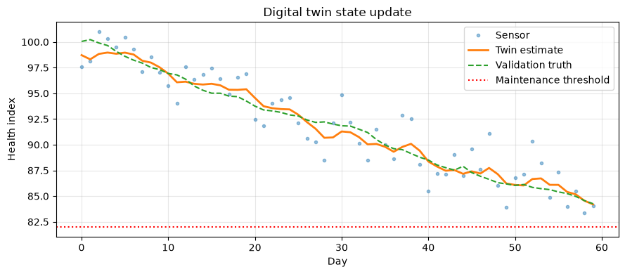
結果の読み取り
生値より安定した推定状態を使うと、閾値付近の誤警報を減らし、保全日程を前倒しで検討できます。実務ではセンサー時刻、校正、欠測、設備改造履歴を管理し、推定値だけで自動停止せず、重要度に応じた承認フローを設けます。
No.100:製造業版Palantirのシミュレーション基盤
実務での意味/分析・モデル化の考え方
最後は個別モデルを、共通の業務オブジェクトと意思決定へ統合します。ここでいう「製造業版Palantir」は特定製品の模倣ではなく、受注・品目・設備・在庫・供給者を意味で結び、シナリオ、根拠、承認、実績を追跡できる基盤の比喩です。
入力→状態→モデル→選択肢→KPI→承認→実績の履歴を残し、同じscenario_idで再計算できる最小構造を確認します。
Pythonで確認する
scenario_catalog=pd.DataFrame([
    ["S-BASE","Baseline",1.00,930,150,"single",0],
    ["S-RES","Resilient",1.08,970,220,"dual",12_000],
    ["S-GROW","Growth",1.18,1050,190,"dual",180_000],
],columns=["scenario_id","name","demand_factor","capacity","safety_stock","sourcing","investment_kJPY"])
def evaluate(row, reps=2000):
    annual_demand=rng.normal(10200*row.demand_factor,1050,reps)
    annual_capacity=rng.normal(row.capacity*12,420,reps)
    shipped=np.minimum(annual_demand+row.safety_stock,annual_capacity)
    disruption=rng.random(reps)<(.025 if row.sourcing=="dual" else .08)
    shipped*=np.where(disruption,.94,1.0)
    service=np.minimum(shipped/annual_demand,1)
    value=shipped*31-row.investment_kJPY-row.safety_stock*.8
    return pd.Series({"expected_value_kJPY":value.mean(),"P(service>=98%)":(service>=.98).mean(),"P(capacity_shortage)":(annual_demand>annual_capacity).mean()})
result_100=pd.concat([scenario_catalog,scenario_catalog.apply(evaluate,axis=1)],axis=1)
display(result_100.round(3))
fig,ax=plt.subplots(figsize=(8,4)); ax.scatter(result_100["P(service>=98%)"]*100,result_100["expected_value_kJPY"]/1000,s=120)
for _,r0 in result_100.iterrows(): ax.annotate(r0["scenario_id"],(r0["P(service>=98%)"]*100,r0["expected_value_kJPY"]/1000),xytext=(5,5),textcoords="offset points")
ax.set(title="Scenario portfolio for integrated decision making",xlabel="Probability of service >= 98% (%)",ylabel="Expected value (million JPY)"); ax.grid(True,alpha=.3); plt.tight_layout(); plt.show()| scenario_id | name | demand_factor | capacity | safety_stock | sourcing | investment_kJPY | expected_value_kJPY | P(service>=98%) | P(capacity_shortage) | |
|---|---|---|---|---|---|---|---|---|---|---|
| 0 | S-BASE | Baseline | 1.00 | 930 | 150 | single | 0 | 314,024.16 | 0.77 | 0.20 |
| 1 | S-RES | Resilient | 1.08 | 970 | 220 | dual | 12000 | 326,979.75 | 0.75 | 0.31 |
| 2 | S-GROW | Growth | 1.18 | 1050 | 190 | dual | 180000 | 189,287.29 | 0.74 | 0.31 |
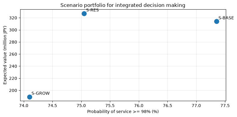
結果の読み取り
統合基盤の価値は、最適解を一つ返すことより、どの入力・モデル・承認で判断し、実績がどうだったかを追跡できる点にあります。導入順序は、経営課題と意思決定周期を定め、共通IDとKPIを整え、小さなシナリオ比較から始めるのが現実的です。
対象ノックを通して見える実務上の示唆
- 平均値ではなく分布で決める:欠品確率、95%点費用、NPV正の確率を見ると、平均ケースでは隠れる脆弱性が分かります。
- 局所最適を避ける:生産量、在庫、人員、調達、設備投資を共通シナリオで評価しなければ、ある部門の改善が別部門の損失になります。
- 制約と目的を分ける:安全、品質、契約サービス水準は重みで相殺せず制約にし、その範囲で利益や在庫を比較します。
- モデルより意思決定プロセスを設計する:入力の責任者、更新頻度、承認者、実績検証、モデル停止条件まで決めて初めて運用になります。
実務導入する場合に必要なこと
- 対象の意思決定、期限、変更可能なレバー、禁止条件を明文化する
- 品目・設備・拠点・サプライヤーの共通IDと、時刻・単位・粒度を統一する
- 過去データで再現性を検証し、現場知識による極端シナリオも試す
- ベースライン、モデル版、入力スナップショット、seed、承認履歴を保存する
- KPIの責任部署と、予測が外れた際の代替運用を決める
- PoCでは精度だけでなく、判断時間、欠品損失、計画変更回数などの業務効果を測る
まとめ
No.091〜No.100では、工場運営の主要な判断を個別シミュレーションから統合シナリオ評価へ段階的につなげました。シミュレーションは現実の完全な複製ではありません。前提を共有し、不確実性を定量化し、選択肢を安全に比較するための「意思決定の実験場」です。小さく検証し、実績との差を学習して更新し続けることが、デジタルツインや統合基盤を現場で生かす近道です。
法人向けのご相談
数理工房では、生産計画・在庫・設備投資・人員配置・サプライチェーンを対象に、課題整理、データ設計、シミュレーションPoC、意思決定基盤への実装・定着化をご支援します。既存のExcelや現場ルールを出発点に、説明可能で運用可能な形へ段階的に整備できます。
📩 お問い合わせ: surikobo.co.jp/contact
まずはお気軽にご相談ください。