Designing Factory Operations Resilient to Fluctuations: Manufacturing Simulation Practice No.091–No.100

Demand, equipment, personnel, inventory, and procurement all influence each other. This notebook uses a fictional precision pump factory as the subject to connect individual optimization calculations to One Decision-Making System in Management and Factory Operations. Through No.091 to No.100, we visualize not only planned values but also volatility, downside risk, investment recovery, and KPI trade-offs.

[!NOTE] This material is a notebook previously used by Surikoubo (or personally by the representative, Kazuyama), and has been reconstructed, edited, and published with the company’s permission.
All data listed is fictional and has no relation whatsoever to real companies, factories, or figures.

Introduction: Practical Challenges in Manufacturing Covered in This Article

Monthly S&OP requires simultaneous alignment of sales plans, production capacity, inventory, purchasing, personnel, and capital investment. However, if you plan based solely on average demand, when demand peaks, breakdowns, and delivery delays pile up, stockouts and overtime can spike. The purpose of this article is not to “guess the future with a single point,” but to compare multiple assumptions in a reproducible way to enhance the robustness of decision-making.

Common situations on site

• Each department has different assumptions and KPIs, and they are not looking at the same scenario.
• Even if a capability enhancement plan is presented, the recovery probability is unknown, including demand fluctuations and startup losses.
• Decisions regarding safety stock, personnel, and outsourcing depend on empirical rules.
• Digital twins stop at visualization and do not connect to plan changes or approvals.

Why is this issue so difficult to judge?

This is because causal relationships circulate. Increasing production increases inventory, but if there is a breakdown or shortage of parts, only work-in-progress increases. Inventory reduction improves working capital but lowers resistance to delivery delays. Therefore, in addition to the average, quantiles, constraints, costs, and service levels are compared using the same model.

Overview of Exercise covered this time

No.	Theme	Key Decisions
091	Production plan	Monthly Production Volume under Demand Fluctuations
092	Factory layout	Reducing transport distances and congestion
093	capital investment	Recoverability of Capacity Enhancements
094	staffing	Staffing under skill constraints
095	Inventory optimization	Order Point and Safety Stock
096	supply chain	Resistance to Procurement Disruptions
097	Demand forecasting and simulation	Planning with Forecast Errors
098	KPI	Balancing profit, delivery time, and inventory
099	Manufacturing Digital Twin	Status updates based on observations
100	The foundation of Palantir’s manufacturing edition	Integration of data, models, and decision-making

Preparing the Python environment

Generate fixed seed random numbers with NumPy, handle tables with pandas, and visualize them with matplotlib. External data, seaborn, and external APIs are not used. Being able to reproduce the same results from the same input and seed is a prerequisite for accountability in meetings and model change management.

import sys
import numpy as np
import pandas as pd
import matplotlib
import matplotlib.pyplot as plt
from IPython.display import display

SEED = 20260712
rng = np.random.default_rng(SEED)
pd.set_option("display.float_format", lambda x: f"{x:,.2f}")
print("Python     :", sys.version.split()[0])
print("NumPy      :", np.__version__)
print("pandas     :", pd.__version__)
print("matplotlib :", matplotlib.__version__)
print("random seed:", SEED)

Python     : 3.13.1
NumPy      : 2.5.1
pandas     : 3.0.3
matplotlib : 3.11.0
random seed: 20260712

Creation of Fictional Data

The target is factories that assemble, inspect, and ship products A, B, and C. We create 12-month standard demand, unit price, coefficient of variation, and process load. Separating data generation from business rules limits the scope of impact when converting data into actual data.

months = pd.date_range("2026-01-01", periods=12, freq="MS")
products = pd.DataFrame({
    "product": ["A", "B", "C"],
    "unit_price_kJPY": [82, 105, 138],
    "unit_margin_kJPY": [31, 39, 52],
    "demand_cv": [0.12, 0.18, 0.25],
    "assembly_h": [0.80, 1.05, 1.35],
    "inspection_h": [0.25, 0.35, 0.50],
})
base = np.array([420, 280, 160])
season = 1 + 0.12 * np.sin(2 * np.pi * (np.arange(12) - 1) / 12)
demand_plan = pd.DataFrame(
    (season[:, None] * base[None, :]).round().astype(int),
    index=months, columns=products["product"]
)
display(products)
display(demand_plan.head())

	product	unit_price_kJPY	unit_margin_kJPY	demand_cv	assembly_h	inspection_h
0	A	82	31	0.12	0.80	0.25
1	B	105	39	0.18	1.05	0.35
2	C	138	52	0.25	1.35	0.50

product	A	B	C
2026-01-01	395	263	150
2026-02-01	420	280	160
2026-03-01	445	297	170
2026-04-01	464	309	177
2026-05-01	470	314	179

No.091: Production Planning Simulation

Meaning in Practice / Approaches to Analysis and Modeling

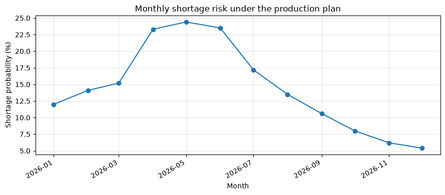
Monthly planning alone meets average demand is not enough. Consider capability caps and beginning inventory to assess the likelihood of stockouts and excess inventory.

The basic relationship between demand $D_t$, production $Q_t$, and ending inventory $I_t$ is $I_t=I_{t-1}+Q_t-D_t$. Areas where inventory is negative are considered out of stock and are simulated multiple times under capacity constraints.

Check with Python

n_sim = 1000
plan_total = demand_plan.sum(axis=1).to_numpy()
demand_total = rng.normal(plan_total, plan_total * 0.16, size=(n_sim, 12)).clip(0)
capacity = 930
production = np.minimum(capacity, plan_total * 1.04)
inventory = np.zeros((n_sim, 13)); inventory[:, 0] = 120
shortage = np.zeros((n_sim, 12))
for t in range(12):
    available = inventory[:, t] + production[t]
    shortage[:, t] = np.maximum(demand_total[:, t] - available, 0)
    inventory[:, t+1] = np.maximum(available - demand_total[:, t], 0)
result_91 = pd.DataFrame({"month": months, "plan": plan_total, "production": production,
                          "median_ending_inventory": np.median(inventory[:,1:], axis=0),
                          "shortage_probability": (shortage > 0).mean(axis=0)})
display(result_91.round(2))
fig, ax = plt.subplots(figsize=(9, 4)); ax.plot(months, result_91["shortage_probability"]*100, marker="o")
ax.set(title="Monthly shortage risk under the production plan", xlabel="Month", ylabel="Shortage probability (%)")
ax.grid(True, alpha=.3); fig.autofmt_xdate(); plt.tight_layout(); plt.show()

/var/folders/3y/fmw40k0x78xblvb3gkcyvy1h0000gn/T/ipykernel_25456/1898123177.py:15: UserWarning: obj.round has no effect with datetime, timedelta, or period dtypes. Use obj.dt.round(...) instead.
  display(result_91.round(2))

	month	plan	production	median_ending_inventory	shortage_probability
0	2026-01-01	808	840.32	151.74	0.12
1	2026-02-01	860	894.40	183.10	0.14
2	2026-03-01	912	930.00	206.32	0.15
3	2026-04-01	950	930.00	188.65	0.23
4	2026-05-01	963	930.00	181.20	0.24
5	2026-06-01	950	930.00	180.24	0.24
6	2026-07-01	912	930.00	204.88	0.17
7	2026-08-01	860	894.40	264.19	0.14
8	2026-09-01	808	840.32	319.11	0.11
9	2026-10-01	770	800.80	353.34	0.08
10	2026-11-01	757	787.28	397.61	0.06
11	2026-12-01	770	800.80	439.14	0.05

Reading the results

Months with a high probability of out-of-stock are not simply a simple increase in production; candidates combine the previous month’s advance production, overtime slots, and outsourcing slots. When the month with median inventory buildup and the month with shortages coexist, it can be interpreted that the issue lies more with monthly capacity allocation than with annual capacity shortfall.

No.092: Factory Layout Simulation

Meaning in Practice / Approaches to Analysis and Modeling

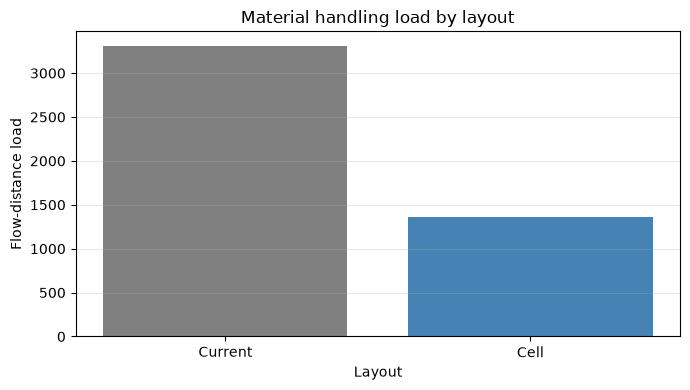
Layout changes involve not only transport distance, but also investment decisions that include aisle congestion, safety, and relocation halts. Here, we compare the transport load between the current draft and the cellulated plan based on inter-process flow and coordinates.

If the number of conveyors between process $i,j$ is $F_{ij}$ and the Manhattan distance is $d_{ij}$, the conveying load is $L=\sum_{i,j}F_{ij}d_{ij}$. Probabilistic wait times that indicate congestion are also included.

Check with Python

flows = {("Receiving","Machining"):80, ("Machining","Assembly"):140, ("Assembly","Inspection"):130, ("Inspection","Shipping"):120}
layouts = {"Current":{"Receiving":(0,0),"Machining":(6,1),"Assembly":(2,6),"Inspection":(7,6),"Shipping":(9,1)},
           "Cell":{"Receiving":(0,0),"Machining":(3,1),"Assembly":(5,2),"Inspection":(7,2),"Shipping":(9,1)}}
rows=[]
for name, pos in layouts.items():
    distance_load=sum(f*(abs(pos[a][0]-pos[b][0])+abs(pos[a][1]-pos[b][1])) for (a,b),f in flows.items())
    congestion=rng.lognormal(mean=np.log(distance_load*0.018), sigma=.18, size=1000)
    rows.append([name,distance_load,np.mean(congestion),np.percentile(congestion,95)])
result_92=pd.DataFrame(rows,columns=["layout","distance_load","mean_delay_min","p95_delay_min"])
display(result_92.round(1))
fig, ax=plt.subplots(figsize=(7,4)); ax.bar(result_92["layout"],result_92["distance_load"],color=["gray","steelblue"])
ax.set(title="Material handling load by layout",xlabel="Layout",ylabel="Flow-distance load"); ax.grid(True,axis="y",alpha=.3); plt.tight_layout(); plt.show()

	layout	distance_load	mean_delay_min	p95_delay_min
0	Current	3310	61.30	81.70
1	Cell	1360	24.90	32.70

Reading the results

If cellulization reduces transport load and 95% delay, it benefits not only average efficiency but also stability during busy times. In actual implementation, fire compartments, maintenance spaces, crossings between forklifts and pedestrians, and production reduction during relocation are added to the constraints.

No.093: Capital Investment Simulation

Meaning in Practice / Approaches to Analysis and Modeling

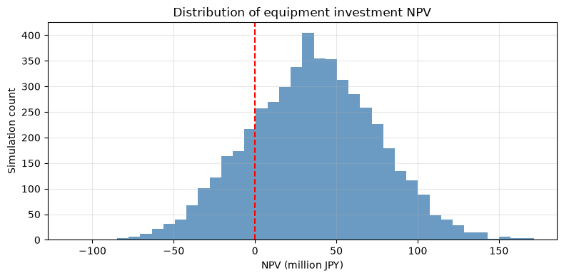
Even if the average NPV is positive, the probability of recovery is high, making decisions more difficult. Evaluate investment proposals by randomly counting demand growth, utilization rates, and startup delays.

$NPV=-C_0+\sum_{t=1}^{T}\frac{CF_t}{(1+r)^t}$ and propagate cash flow uncertainty using the Monte Carlo method.

Check with Python

n=5000; years=np.arange(1,6); investment=180_000; discount=.08
growth=rng.normal(.045,.035,n); uptime=rng.beta(35,3,n); ramp_delay=rng.choice([0,1,2],n,p=[.65,.25,.10])
npvs=np.full(n,-investment,dtype=float)
for y in years:
    volume=4200*(1+growth)**y*uptime
    volume=np.where(y<=ramp_delay,volume*.55,volume)
    cash=volume*18-22_000
    npvs += cash/(1+discount)**y
result_93=pd.Series({"mean_NPV_kJPY":npvs.mean(),"median_NPV_kJPY":np.median(npvs),"P(NPV>0)":(npvs>0).mean(),"P10_NPV_kJPY":np.percentile(npvs,10)})
display(result_93.to_frame("value").round(2))
fig,ax=plt.subplots(figsize=(8,4)); ax.hist(npvs/1000,bins=40,color="steelblue",alpha=.8); ax.axvline(0,color="red",linestyle="--")
ax.set(title="Distribution of equipment investment NPV",xlabel="NPV (million JPY)",ylabel="Simulation count"); ax.grid(True,alpha=.3); plt.tight_layout(); plt.show()

	value
mean_NPV_kJPY	35,512.67
median_NPV_kJPY	35,614.25
P(NPV>0)	0.81
P10_NPV_kJPY	-16,809.36

Reading the results

In the selection decision, we look not only at the average NPV but also at the probability of positive NPV and the bottom 10%. If there is a large downside, risk reduction measures such as converting lump-sum investments into phased investments, securing demand contracts before placing orders, or including startup support as contract terms are compared among other risk mitigation measures.

No.094: Staffing Simulation

Meaning in Practice / Approaches to Analysis and Modeling

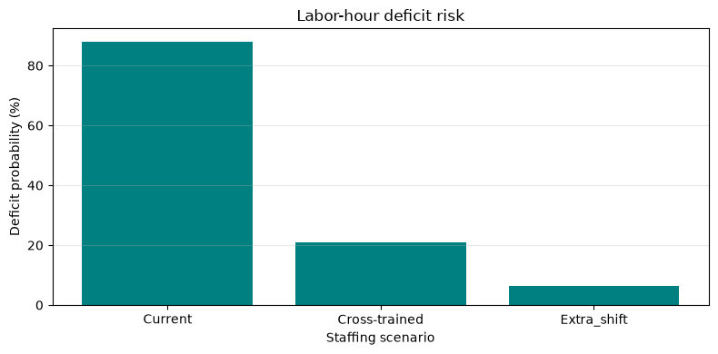
Even if you have enough people, if the required skills don’t match, the line won’t work. Comparing staffing including assembly and inspection skill proficiency, absenteeism, and support potential.

The difference between required and supplied man-hours is called the shortfall, and absenteeism is reproduced using the Bernoulli trial. Multi-skilled workers are evaluated not as a measure to increase the number of people but to enhance skill substitutability.

Check with Python

scenarios={"Current":(.08,.55),"Cross-trained":(.08,.80),"Extra_shift":(.05,.85)}
rows=[]
for name,(absence,qualified) in scenarios.items():
    present=rng.binomial(24,1-absence,2000)
    skilled=rng.binomial(present,qualified)
    supplied=skilled*7.2
    required=rng.normal(112,12,2000)
    deficit=np.maximum(required-supplied,0)
    rows.append([name,deficit.mean(),np.percentile(deficit,95),(deficit>0).mean()])
result_94=pd.DataFrame(rows,columns=["scenario","mean_deficit_h","p95_deficit_h","deficit_probability"])
display(result_94.round(2))
fig,ax=plt.subplots(figsize=(8,4)); ax.bar(result_94["scenario"],result_94["deficit_probability"]*100,color="teal")
ax.set(title="Labor-hour deficit risk",xlabel="Staffing scenario",ylabel="Deficit probability (%)"); ax.grid(True,axis="y",alpha=.3); plt.tight_layout(); plt.show()

	scenario	mean_deficit_h	p95_deficit_h	deficit_probability
0	Current	25.51	59.40	0.88
1	Cross-trained	2.46	17.72	0.21
2	Extra_shift	0.66	2.82	0.06

Reading the results

If the probability of shortages drops significantly due to multi-skilled work, investment in education may be more effective than constant increases. However, treating skills with binary values is simplified. In practice, qualifications, validity periods, proficiency levels, instructors, continuous working hours, and personal preferences are all constraints for management.

No.095: Inventory Optimization Simulation

Meaning in Practice / Approaches to Analysis and Modeling

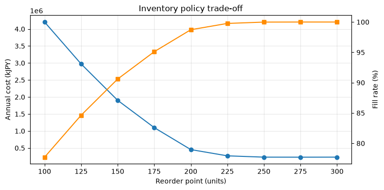
Safety stock prevents stockouts while increasing storage costs and the risk of obsolescence. Simulate candidate order points and compare service levels with total costs.

The order point is generally $ROP=\mu_L+z\sigma_L$. However, due to lead time fluctuations and lot restrictions, daily inventory trends are directly reproduced.

Check with Python

def inventory_policy(rop, days=365, reps=300):
    costs=[]; fill=[]
    for _ in range(reps):
        inv=rop+180; on_order=[]; demand_total=served=holding=orders=0
        for day in range(days):
            inv += sum(q for due,q in on_order if due==day); on_order=[x for x in on_order if x[0]>day]
            d=max(0,int(rng.normal(28,7))); demand_total+=d; s=min(inv,d); served+=s; inv-=s; holding+=inv
            if inv+sum(q for _,q in on_order)<=rop:
                on_order.append((day+int(rng.integers(4,9)),180)); orders+=1
        costs.append(holding*.12+orders*4_000+(demand_total-served)*1_800); fill.append(served/demand_total)
    return np.mean(costs),np.mean(fill)
result_95=pd.DataFrame([(r,*inventory_policy(r)) for r in range(100,301,25)],columns=["reorder_point","annual_cost_kJPY","fill_rate"])
display(result_95.round(3))
fig,ax1=plt.subplots(figsize=(8,4)); ax1.plot(result_95["reorder_point"],result_95["annual_cost_kJPY"],marker="o",label="Cost")
ax1.set(title="Inventory policy trade-off",xlabel="Reorder point (units)",ylabel="Annual cost (kJPY)"); ax1.grid(True,alpha=.3)
ax2=ax1.twinx(); ax2.plot(result_95["reorder_point"],result_95["fill_rate"]*100,color="darkorange",marker="s",label="Fill rate"); ax2.set_ylabel("Fill rate (%)"); plt.tight_layout(); plt.show()

	reorder_point	annual_cost_kJPY	fill_rate
0	100	4,205,229.20	0.78
1	125	2,972,266.99	0.85
2	150	1,902,245.51	0.91
3	175	1,099,789.77	0.95
4	200	453,631.91	0.99
5	225	269,555.54	1.00
6	250	231,186.30	1.00
7	275	230,062.74	1.00
8	300	231,307.18	1.00

Reading the results

The basic approach is to select the order point with the lowest total cost from among candidates that meet the minimum service level. Since out-of-stock losses differ between critical customer parts and generic products, it is necessary to agree on service levels for each item rather than a uniform inventory period for all items.

No.096: Supply Chain Simulation

Meaning in Practice / Approaches to Analysis and Modeling

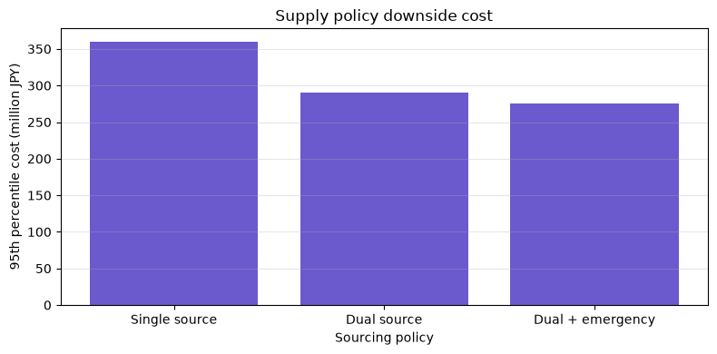
A low-priced single procurement is not necessarily cheap, including losses during interruptions. Compare the annual total costs and number of downtime for single procurement, two-company purchasing, and emergency procurement.

Costs for operating downtime due to delays or interruptions are added to the expected procurement costs. It is important not to overlook correlated disaster risks and regional dependence.

Check with Python

policies={"Single source":(1.00,.08,0),"Dual source":(1.06,.025,0),"Dual + emergency":(1.10,.012,6000)}
rows=[]
for name,(price_factor,disrupt_p,emergency) in policies.items():
    costs=[]; stops=[]
    for _ in range(3000):
        disrupted=rng.random(12)<disrupt_p; stop_days=(rng.integers(2,12,12)*disrupted).sum()
        procurement=12*15_000*price_factor; total=procurement+stop_days*9_000+emergency*(stop_days>0)
        costs.append(total); stops.append(stop_days)
    rows.append([name,np.mean(costs),np.percentile(costs,95),np.mean(stops),(np.array(stops)>0).mean()])
result_96=pd.DataFrame(rows,columns=["policy","mean_cost_kJPY","p95_cost_kJPY","mean_stop_days","disruption_probability"])
display(result_96.round(2))
fig,ax=plt.subplots(figsize=(8,4)); ax.bar(result_96["policy"],result_96["p95_cost_kJPY"]/1000,color="slateblue")
ax.set(title="Supply policy downside cost",xlabel="Sourcing policy",ylabel="95th percentile cost (million JPY)"); ax.grid(True,axis="y",alpha=.3); plt.tight_layout(); plt.show()

	policy	mean_cost_kJPY	p95_cost_kJPY	mean_stop_days	disruption_probability
0	Single source	235,824.00	360,000.00	6.20	0.61
1	Dual source	207,753.00	289,800.00	1.88	0.25
2	Dual + emergency	207,448.00	276,000.00	0.96	0.14

Reading the results

Even if the two-company purchase price is raised during normal hours, it can reduce total costs and downtime by 95%. In BCP assessment, we check not only expected costs but also the maximum allowable downtime duration, the certification period for substitute materials, the location of molds and jigs, and even secondary suppliers for suppliers.

No.097: Demand Forecasting and Simulation

Meaning in Practice / Approaches to Analysis and Modeling

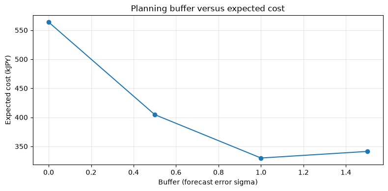
If you place the forecast value directly in the production plan, you ignore the forecast error. Separate point prediction and error distribution, and compare planned buffers including upward and downward bias.

$y_t$ performance, $\hat y_t$ forecasts, and resample error $e_t=y_t-\hat y_t$. Not only MAE but also shortage and inventory costs that propagated errors to the plan are used to make judgments.

Check with Python

history_actual=700+35*np.sin(np.arange(36)*2*np.pi/12)+rng.normal(0,55,36)
history_forecast=700+35*np.sin(np.arange(36)*2*np.pi/12)
errors=history_actual-history_forecast
future_forecast=700+35*np.sin(np.arange(36,48)*2*np.pi/12)
buffers=[0,.5,1.0,1.5]; rows=[]
for z in buffers:
    plan=future_forecast+z*errors.std()
    simulated=future_forecast+rng.choice(errors,size=(3000,12),replace=True)
    shortage=np.maximum(simulated-plan,0).sum(axis=1); excess=np.maximum(plan-simulated,0).sum(axis=1)
    cost=shortage*2.4+excess*.35
    rows.append([z,cost.mean(),(shortage==0).mean(),shortage.mean(),excess.mean()])
result_97=pd.DataFrame(rows,columns=["buffer_sigma","mean_cost_kJPY","no_shortage_probability","mean_shortage","mean_excess"])
display(result_97.round(2))
fig,ax=plt.subplots(figsize=(8,4)); ax.plot(result_97["buffer_sigma"],result_97["mean_cost_kJPY"],marker="o")
ax.set(title="Planning buffer versus expected cost",xlabel="Buffer (forecast error sigma)",ylabel="Expected cost (kJPY)"); ax.grid(True,alpha=.3); plt.tight_layout(); plt.show()

	buffer_sigma	mean_cost_kJPY	no_shortage_probability	mean_shortage	mean_excess
0	0.00	563.81	0.01	193.48	284.18
1	0.50	404.55	0.01	99.52	473.42
2	1.00	329.96	0.16	35.26	700.96
3	1.50	341.27	0.51	1.58	964.23

Reading the results

Even if forecasting accuracy is the same, the appropriate buffer will differ depending on the ratio of out-of-stock costs to inventory costs. If there is bias in the forecasting error, the forecasting process is corrected before adding buffers. It is also essential to unify the meaning of observations such as promotions, lost orders, and backlog orders.

No.098: KPI Simulation

Meaning in Practice / Approaches to Analysis and Modeling

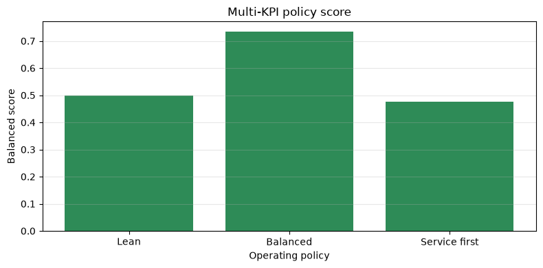
Maximizing a single KPI can cause side effects. High utilization rates can worsen work-in-progress and delivery times, while inventory reductions increase shortages. Compare KPIs for each driving policy under the same scenario.

Profit, OTIF (On-Time to Quantity Delivery Rate), inventory turnover, and overtime are normalized and scored. However, weight is a management decision, not automatically determined by the model.

Check with Python

policies=[("Lean",.96,.92,10.2,140), ("Balanced",.985,.97,8.4,210), ("Service first",.995,.985,6.3,330)]
rows=[]
for name,yield_rate,otif,turns,overtime in policies:
    profit=420_000*yield_rate + 95_000*otif + rng.normal(0,8000,1500)-overtime*55
    rows.append([name,profit.mean(),otif,turns,overtime])
result_98=pd.DataFrame(rows,columns=["policy","expected_profit_kJPY","OTIF","inventory_turns","overtime_h"])
for c in ["expected_profit_kJPY","OTIF","inventory_turns"]:
    result_98[c+"_score"]=(result_98[c]-result_98[c].min())/(result_98[c].max()-result_98[c].min())
result_98["overtime_score"]=1-(result_98["overtime_h"]-result_98["overtime_h"].min())/(result_98["overtime_h"].max()-result_98["overtime_h"].min())
result_98["balanced_score"]=result_98[["expected_profit_kJPY_score","OTIF_score","inventory_turns_score","overtime_score"]].mean(axis=1)
display(result_98[["policy","expected_profit_kJPY","OTIF","inventory_turns","overtime_h","balanced_score"]].round(3))
fig,ax=plt.subplots(figsize=(8,4)); ax.bar(result_98["policy"],result_98["balanced_score"],color="seagreen")
ax.set(title="Multi-KPI policy score",xlabel="Operating policy",ylabel="Balanced score"); ax.grid(True,axis="y",alpha=.3); plt.tight_layout(); plt.show()

	policy	expected_profit_kJPY	OTIF	inventory_turns	overtime_h	balanced_score
0	Lean	483,023.36	0.92	10.20	140	0.50
1	Balanced	494,383.01	0.97	8.40	210	0.73
2	Service first	493,255.15	0.98	6.30	330	0.47

Reading the results

Even if a balanced proposal has an overall advantage, any proposal below the minimum OTIF standard should be disqualified. Weighted averages are for explanatory purposes and must not offset restrictions on laws, safety, quality assurance, or customer contracts. Sensitivity analysis and weight agreement at management meetings are necessary.

No.099: Construction of a Digital Twin for the Manufacturing Industry

Meaning in Practice / Approaches to Analysis and Modeling

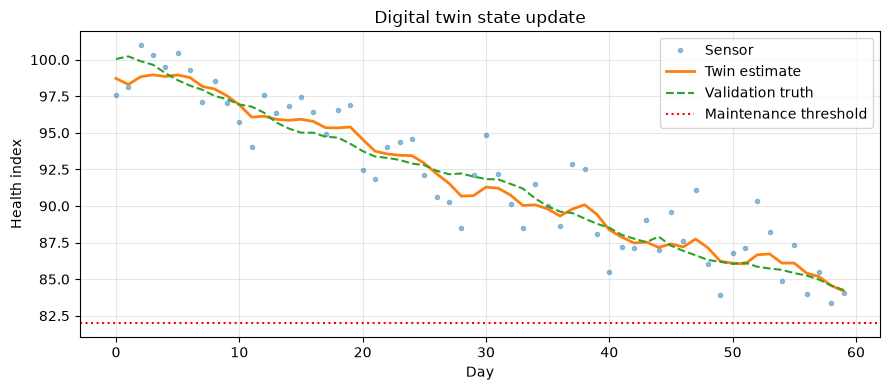
Digital twins are not 3D displays; instead, they update the model’s state through real-world observations, predicting the future and leading to action. Here, the deterioration of the equipment is sequentially corrected using sensor values.

If we $x_t^-$ the forecast state and the observation $y_t$, the update is $x_t=x_t^-+K_t(y_t-x_t^-)$. A simple one-dimensional Kalman filter tracks degradation while leveling out observation noise.

Check with Python

days=np.arange(60); true_health=100-.32*days+np.cumsum(rng.normal(0,.18,60)); sensor=true_health+rng.normal(0,2.2,60)
estimate=[]; x=100.; p=4.; q=.25; r=2.2**2
for y in sensor:
    x_pred=x-.32; p_pred=p+q; k=p_pred/(p_pred+r); x=x_pred+k*(y-x_pred); p=(1-k)*p_pred; estimate.append(x)
result_99=pd.DataFrame({"day":days,"sensor":sensor,"estimated_health":estimate,"true_health_for_validation":true_health})
display(result_99.tail().round(2))
fig,ax=plt.subplots(figsize=(9,4)); ax.plot(days,sensor,".",alpha=.45,label="Sensor"); ax.plot(days,estimate,label="Twin estimate",linewidth=2); ax.plot(days,true_health,"--",label="Validation truth")
ax.axhline(82,color="red",linestyle=":",label="Maintenance threshold"); ax.set(title="Digital twin state update",xlabel="Day",ylabel="Health index"); ax.grid(True,alpha=.3); ax.legend(); plt.tight_layout(); plt.show()

	day	sensor	estimated_health	true_health_for_validation
55	55	87.34	86.10	85.41
56	56	83.99	85.41	85.25
57	57	85.49	85.17	84.97
58	58	83.38	84.55	84.56
59	59	84.04	84.19	84.26

Reading the results

Using estimation conditions that are more stable than raw values reduces false alarms near thresholds and allows for earlier consideration of maintenance schedules. In practice, we manage sensor time, calibration, missing measurements, and equipment modification history, and instead of automatically stopping based on estimates, we establish approval flows based on importance.

No.100: Manufacturing Version of Palantir’s Simulation Platform

Meaning in Practice / Approaches to Analysis and Modeling

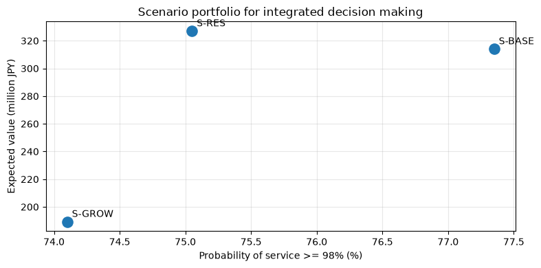
Finally, we integrate individual models into common business objects and decision-making. Here, the “manufacturing version of Palantir” does not refer to imitation of specific products, but rather to a metaphor for the platform that connects orders, items, equipment, inventory, and suppliers, allowing for tracking scenarios, grounds, approvals, and performance.

Input → status → model → options → keep a history of KPI→ approval→ and confirm the minimum structure that can be recalculated on the same scenario_id.

Check with Python

scenario_catalog=pd.DataFrame([
    ["S-BASE","Baseline",1.00,930,150,"single",0],
    ["S-RES","Resilient",1.08,970,220,"dual",12_000],
    ["S-GROW","Growth",1.18,1050,190,"dual",180_000],
],columns=["scenario_id","name","demand_factor","capacity","safety_stock","sourcing","investment_kJPY"])
def evaluate(row, reps=2000):
    annual_demand=rng.normal(10200*row.demand_factor,1050,reps)
    annual_capacity=rng.normal(row.capacity*12,420,reps)
    shipped=np.minimum(annual_demand+row.safety_stock,annual_capacity)
    disruption=rng.random(reps)<(.025 if row.sourcing=="dual" else .08)
    shipped*=np.where(disruption,.94,1.0)
    service=np.minimum(shipped/annual_demand,1)
    value=shipped*31-row.investment_kJPY-row.safety_stock*.8
    return pd.Series({"expected_value_kJPY":value.mean(),"P(service>=98%)":(service>=.98).mean(),"P(capacity_shortage)":(annual_demand>annual_capacity).mean()})
result_100=pd.concat([scenario_catalog,scenario_catalog.apply(evaluate,axis=1)],axis=1)
display(result_100.round(3))
fig,ax=plt.subplots(figsize=(8,4)); ax.scatter(result_100["P(service>=98%)"]*100,result_100["expected_value_kJPY"]/1000,s=120)
for _,r0 in result_100.iterrows(): ax.annotate(r0["scenario_id"],(r0["P(service>=98%)"]*100,r0["expected_value_kJPY"]/1000),xytext=(5,5),textcoords="offset points")
ax.set(title="Scenario portfolio for integrated decision making",xlabel="Probability of service >= 98% (%)",ylabel="Expected value (million JPY)"); ax.grid(True,alpha=.3); plt.tight_layout(); plt.show()

	scenario_id	name	demand_factor	capacity	safety_stock	sourcing	investment_kJPY	expected_value_kJPY	P(service>=98%)	P(capacity_shortage)
0	S-BASE	Baseline	1.00	930	150	single	0	314,024.16	0.77	0.20
1	S-RES	Resilient	1.08	970	220	dual	12000	326,979.75	0.75	0.31
2	S-GROW	Growth	1.18	1050	190	dual	180000	189,287.29	0.74	0.31

Reading the results

The value of the integrated platform lies not in providing a single optimal solution, but in being able to track performance by making judgments based on inputs, models, and approvals. The implementation sequence is to define management issues and decision-making cycles, establish common IDs and KPIs, and start with small-scale scenario comparisons.

Practical Implications Seen Through Target Exercise

1. Determined by distribution, not average: Looking at out-of-stock probability, 95% point cost, and NPV positive probability, you can see hidden vulnerabilities in average cases.
2. Avoiding local optimization: If production volume, inventory, personnel, procurement, and capital investment are not evaluated under common scenarios, improvements in one department may result in losses for another.
3. Separate constraints from objectives: Safety, quality, and contracted service levels should not be offset by weights but constrained by constraints, and profits and inventory should be compared within that range.
4. Designing the decision-making process beyond the model: Operation only begins after deciding the person responsible for input, update frequency, approver, performance verification, and even the conditions for model stoppage.

What is necessary for practical implementation

• Clearly state the subject decision-making, deadlines, changeable levers, and prohibitive conditions
• Standardize common IDs for items, equipment, bases, and suppliers, as well as time, units, and granularity
• Verifying reproducibility with past data and testing extreme scenarios based on on-site knowledge
• Save baselines, model versions, input snapshots, seeds, and approval history
• Decide on the KPI responsible department and alternative operations if predictions are wrong.
• PoC measures not only accuracy but also operational effectiveness such as decision time, out-of-stock losses, and the number of plan changes

Conclusion

From No.091 to No.100, key decisions in factory operations were gradually connected from individual simulations to integrated scenario evaluations. Simulation is not a complete replica of reality. It serves as a “testing ground for decision-making” to share assumptions, quantify uncertainty, and safely compare options. Conducting small-scale verification, learning from differences from actual performance, and continuously updating is the shortcut to leveraging digital twins and integrated infrastructure in the field.

Consultations for Corporations

At Suri Kobo, we support issue organization, data design, simulation PoC, and implementation and embedding in decision-making platforms, covering production planning, inventory, capital investment, personnel allocation, and supply chain. Starting from existing Excel and on-site rules, you can gradually develop it into an explainable and operable form.

📩 Contact Us: surikobo.co.jp/contact
Please feel free to consult us first.