How to determine investment and operational conditions for multi-product assembly lines

From “Proposals with Good Averages” to “Usable On-Site Solutions” through Simulation Optimization (No.081–No.090)

Using the multi-variety assembly line subject to demand fluctuations, equipment shutdowns, and setup changes, it deals with how to determine Personnel, intermediate buffers, and preventive maintenance intervals. Not only a single forecast but also profit, on-time delivery rate, work-in-progress (WIP), and downtime risk are simultaneously examined, step-by-step verification of exploration methods and decision-making processes.

[!NOTE] This material is a notebook previously used by Surikoubo (or personally by the representative, Kazuyama), and has been reconstructed, edited, and published with the company’s permission.
All data listed is fictional and has no relation whatsoever to real companies, factories, or figures.

1. Introduction: Practical Challenges in Manufacturing Covered in This Article

There is no single way to increase production capacity. Increasing staff, expanding buffers, and reviewing maintenance frequency each improve capacity while increasing labor, inventory, and maintenance costs. Moreover, demand and breakdowns occur probabilistically, so plans decided solely on average demand may fall apart on busy or outage days.

The decisions made in this paper are organized under the following constrained objectives.

$$\max_x\; \mathbb{E}[\Pi(x,\xi)] \quad \text{s.t.}\quad P\{S(x,\xi) \geq 0.95\} \text{emphasis on value},\; x \in \mathcal{X}$$

$x$ is the number of personnel, buffer capacity, and maintenance intervals; $\xi$ is uncertainties such as demand and breakdowns; $\Pi$ is daily profit; $S$ is the delivery on-time rate. We do not only maximize expected profits, but also list service levels and downsides.

2. Common Situations on Site

• Each department evaluates proposals with separate KPIs, and there is no comparison table for overall optimization.
• Capacity plans created on past averages are unable to withstand demand fluctuations or equipment shutdowns.
• There are many candidate improvement proposals, and actual machine testing of all combinations is not possible.
• I created simulations, but they haven’t led to optimization, performance updates, or approval.

3. Why is this issue difficult to judge?

The simulation output contains random errors, and the objective function is not always smooth. Furthermore, proposals with higher average profits and stable on-time delivery rates may not always match. Rather than simply adopting the results of search algorithms, it is necessary to check constraints, reproducibility, and robustness across multiple scenarios.

4. The overall picture of exercise covered this time

No.	Theme	Decision-Making Role
081	Simulation optimization	Defining objectives, variables, constraints, and random numbers
082	Grid Search	Create easy-to-explain candidate comparisons
083	Genetic algorithm	Exploring a wide discrete space collectively
084	annealing method	Performing neighborhood searches to escape local solutions
085	Bayesian optimization	Finding promising conditions with fewer trials
086	Introduction to Optuna	Establishing search history and reproducible implementations
087	Mathematical optimization × simulation	Share scenario evaluation and resource allocation
088	Integration with Reinforcement Learning	Learn operational rules according to the condition
089	Digital twin	Continuously updating models with achievements
090	What-if Analysis	Comparing robustness by management scenario

5. Preparing the Python environment

Pass the random number generator as an argument so that the same seed can be reproduced with the same result. All graphs are created in matplotlib.

import logging
import warnings

import numpy as np
import pandas as pd
import matplotlib.pyplot as plt
import japanize_matplotlib
from scipy.optimize import milp, LinearConstraint, Bounds
from scipy.stats import norm
from sklearn.gaussian_process import GaussianProcessRegressor
from sklearn.gaussian_process.kernels import Matern, WhiteKernel

warnings.filterwarnings("ignore")
pd.set_option("display.max_columns", 20)
BASE_SEED = 1609
print("NumPy:", np.__version__)
print("pandas:", pd.__version__)

NumPy: 2.5.1
pandas: 3.0.3

6. Creation of Fictional Data

One trial per day is generated, demand is generated based on a normal distribution, and sudden downtime is generated based on an exponential distribution. Personnel workers refers to processing capacity, buffer refers to flow congestion, and pm_interval is a simplified model affecting failure risk and maintenance costs. This is not a model that faithfully replicates the physical behavior of equipment, but rather a proxy model for learning the decision-making process.

def simulate_policy(workers, buffer, pm_interval, n_days=240, seed=BASE_SEED,
                    demand_mean=112, failure_scale=1.0):
    rng = np.random.default_rng(seed)
    demand = np.maximum(60, rng.normal(demand_mean, 18, n_days)).round()
    failure_prob = np.clip(0.025 + 0.00045 * (pm_interval - 20) ** 1.35, 0.02, 0.24)
    failure = rng.random(n_days) < failure_prob
    downtime = failure * rng.exponential(2.7 * failure_scale, n_days)
    variation = rng.normal(0, 4, n_days)
    nominal_capacity = 79 + 8.3 * workers + 1.7 * np.sqrt(buffer)
    capacity = np.maximum(0, nominal_capacity + variation - 5.8 * downtime)
    shipped = np.minimum(demand, capacity)
    shortage = demand - shipped
    wip = np.minimum(buffer, np.maximum(0, demand - 0.84 * capacity))
    revenue = 1.65 * shipped
    cost = (0.40 * shipped + 11.5 * workers + 0.075 * buffer
            + 84 / pm_interval + 1.8 * downtime + 2.9 * shortage + 0.055 * wip)
    profit = revenue - cost
    return pd.DataFrame({
        "demand": demand, "shipped": shipped, "shortage": shortage,
        "wip": wip, "downtime_h": downtime, "profit_10k_yen": profit,
        "on_time": shortage <= 2,
    })

def evaluate_policy(workers, buffer, pm_interval, n_days=240, seed=BASE_SEED,
                    demand_mean=112, failure_scale=1.0):
    d = simulate_policy(workers, buffer, pm_interval, n_days, seed,
                        demand_mean, failure_scale)
    return {
        "workers": workers, "buffer": buffer, "pm_interval": pm_interval,
        "mean_profit": d["profit_10k_yen"].mean(),
        "p05_profit": d["profit_10k_yen"].quantile(0.05),
        "on_time_rate": d["on_time"].mean(),
        "mean_wip": d["wip"].mean(),
        "downtime_h": d["downtime_h"].mean(),
    }

baseline_daily = simulate_policy(4, 30, 45)
baseline = pd.DataFrame([evaluate_policy(4, 30, 45)]).round(2)
baseline

	workers	buffer	pm_interval	mean_profit	p05_profit	on_time_rate	mean_wip	downtime_h
0	4	30	45	69.48	24.19	0.67	13.61	0.17

fig, axes = plt.subplots(1, 2, figsize=(11, 3.8))
axes[0].plot(baseline_daily.index[:60], baseline_daily["demand"][:60], label="need")
axes[0].plot(baseline_daily.index[:60], baseline_daily["shipped"][:60], label="Shipping")
axes[0].set_title("Draft standards: The first60Daily Trends in Days")
axes[0].set_xlabel("days")
axes[0].set_ylabel("Quantity (pieces)/Day)")
axes[0].grid(True, alpha=.3)
axes[0].legend()
axes[1].hist(baseline_daily["profit_10k_yen"], bins=20, edgecolor="white")
axes[1].axvline(baseline_daily["profit_10k_yen"].quantile(.05), color="red", linestyle="--", label="5%point")
axes[1].set_title("Standard: Distribution of Daily Earnings")
axes[1].set_xlabel("Profit (ten thousand yen)/Day)")
axes[1].set_ylabel("number of days")
axes[1].grid(True, alpha=.3)
axes[1].legend()
plt.tight_layout()
plt.show()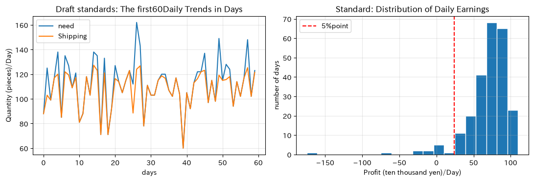

No.081: What is Simulation Optimization?

Meaning in Practice

Simulation optimization is a framework that evaluates numerous equipment and personnel conditions that cannot be tested in reality in a virtual factory and searches for desirable solutions. The important thing is not to “use optimization software,” but to agree on decision variables, evaluation KPIs, and constraints to be followed.

Approach to Analysis and Modeling

Here, a score with a high penalty for a delivery rate below 95% is used.

$J(x)=E[\Pi]-300\max(0,0.95-E[S])-0.15E[WIP]$

The coefficient of 300 reflects management decisions and is not a statistically automatically determined value.

Check with Python

def business_score(row):
    return row["mean_profit"] - 300 * max(0, .95 - row["on_time_rate"]) - .15 * row["mean_wip"]

candidates_081 = [(4, 30, 45), (5, 30, 45), (4, 50, 30), (5, 50, 30)]
result_081 = pd.DataFrame([evaluate_policy(*x, seed=8100+i) for i, x in enumerate(candidates_081)])
result_081["score"] = result_081.apply(business_score, axis=1)
result_081.sort_values("score", ascending=False).round(2)

	workers	buffer	pm_interval	mean_profit	p05_profit	on_time_rate	mean_wip	downtime_h	score
3	5	50	30	69.57	39.39	0.87	8.33	0.02	43.32
1	5	30	45	68.61	31.82	0.80	10.00	0.21	22.11
2	4	50	30	75.09	37.45	0.74	12.95	0.04	9.40
0	4	30	45	74.24	28.65	0.71	13.29	0.10	-0.26

Reading the results

Not only average profit, but also on-time delivery rates and 5% profit points differ for each candidate. Since the top scorer depends on “what was emphasized,” the penalty coefficient and service level are agreed upon among production, sales, and accounting before hiring.

No.082: Grid Search

Meaning in Practice

For equipment specifications and work arrangements with few options, grid searches covering candidates are easier to explain during audits and approvals.

Approach to Analysis and Modeling

Candidates for dispersal are 4 to 6 personnel, 20 to 60 buffers, and maintenance intervals of 20 to 60 days. Ideally, the same candidate would be evaluated using multiple random number series, but for simplicity, we will evaluate each candidate over 240 days.

Check with Python

grid_rows = []
for w in range(4, 7):
    for b in range(20, 61, 10):
        for pm in range(20, 61, 10):
            row = evaluate_policy(w, b, pm, seed=8200 + w*100 + b + pm)
            row["score"] = business_score(row)
            grid_rows.append(row)
grid = pd.DataFrame(grid_rows).sort_values("score", ascending=False).reset_index(drop=True)
grid.head(8).round(2)

	workers	buffer	pm_interval	mean_profit	p05_profit	on_time_rate	mean_wip	downtime_h	score
0	6	50	30	63.87	29.45	0.95	4.83	0.05	63.14
1	6	40	40	64.77	30.90	0.95	5.39	0.11	62.71
2	6	60	60	65.68	33.85	0.94	5.29	0.11	62.38
3	6	60	20	61.98	27.30	0.97	4.43	0.04	61.31
4	6	60	40	64.74	30.46	0.94	5.51	0.13	60.17
5	6	30	50	65.14	32.07	0.93	5.98	0.17	59.24
6	6	60	30	59.40	23.64	0.95	4.87	0.17	58.67
7	6	50	20	59.75	24.73	0.95	4.78	0.02	57.78

pivot = grid.groupby(["workers", "buffer"], as_index=False)["score"].max().pivot(index="workers", columns="buffer", values="score")
fig, ax = plt.subplots(figsize=(7, 3.8))
im = ax.imshow(pivot.values, aspect="auto", cmap="viridis")
ax.set_xticks(range(len(pivot.columns)), pivot.columns)
ax.set_yticks(range(len(pivot.index)), pivot.index)
ax.set_title("Grid Search: Highest scores by personnel and buffer")
ax.set_xlabel("Buffer capacity (units)")
ax.set_ylabel("Personnel (persons)")
ax.grid(False)
fig.colorbar(im, ax=ax, label="Score")
plt.tight_layout()
plt.show()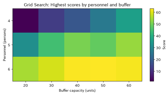

Reading the results

From the top table, it is clear that increasing staff is not always beneficial; profitability changes depending on the combination of buffers and maintenance intervals. If the number of candidates ranges from several thousand to several million, switch to the next probabilistic search.

No.083: Genetic Algorithm

Meaning in Practice

When there is a wide combination of discrete variables such as layout, equipment type, and personnel, the genetic algorithm (GA) can improve multiple candidates in parallel.

Approach to Analysis and Modeling

Candidates are regarded as gene [workers, buffer, pm_interval], and selection, crossbreeding, and mutations are repeated. Since it is impossible to prove optimality, multiple seeds and re-evaluation of final candidates are necessary.

Check with Python

def clip_gene(g):
    return np.array([np.clip(round(g[0]), 3, 7), np.clip(round(g[1]/5)*5, 10, 80),
                     np.clip(round(g[2]/5)*5, 15, 75)], dtype=int)

rng = np.random.default_rng(8300)
pop = np.column_stack([rng.integers(3, 8, 18), rng.integers(2, 17, 18)*5, rng.integers(3, 16, 18)*5])
ga_history = []
for gen in range(16):
    scored = []
    for i, g in enumerate(pop):
        r = evaluate_policy(*g, n_days=160, seed=83000 + gen*100 + i)
        scored.append((business_score(r), g.copy()))
    scored.sort(key=lambda z: z[0], reverse=True)
    ga_history.append(scored[0][0])
    elite = [g for _, g in scored[:6]]
    children = elite.copy()
    while len(children) < len(pop):
        a, b = rng.choice(len(elite), 2, replace=False)
        child = np.where(rng.random(3) < .5, elite[a], elite[b]).astype(float)
        if rng.random() < .45:
            child += rng.choice([[1,0,0],[-1,0,0],[0,5,0],[0,-5,0],[0,0,5],[0,0,-5]])
        children.append(clip_gene(child))
    pop = np.array(children)
ga_best = scored[0][1]
pd.DataFrame([evaluate_policy(*ga_best, n_days=1000, seed=83999)]).round(2)

	workers	buffer	pm_interval	mean_profit	p05_profit	on_time_rate	mean_wip	downtime_h
0	6	70	40	60.61	22.4	0.96	3.57	0.11

plt.figure(figsize=(7, 3.5))
plt.plot(range(1, len(ga_history)+1), ga_history, marker="o")
plt.title("Trends in Genetic Algorithm Exploration")
plt.xlabel("generation")
plt.ylabel("Highest scores within a generation")
plt.grid(True, alpha=.3)
plt.tight_layout()
plt.show()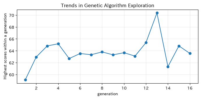

Reading the results

They move into promising areas by generation, but the ups and downs along the way also include the effects of simulation noise. The final proposal will be re-evaluated after 1,000 days, and high scores during exploration will not be adopted.

No.084: Annealing Method

Meaning in Practice

In improvement activities that only slightly change conditions from the current proposal, the approach of “testing the neighborhood plan” under the Annealing Act (SA) is natural.

Approach to Analysis and Modeling

Not only improvement proposals, but also deterioration proposals based on temperature $T$ are accepted with a $\exp(\{\Delta J/T\})$ probability, aiming to escape from local solutions. How the temperature is lowered and the definition of proximity determine the outcome.

Check with Python

rng = np.random.default_rng(8400)
current = np.array([4, 30, 45])
current_score = business_score(evaluate_policy(*current, n_days=180, seed=84000))
best, best_score = current.copy(), current_score
sa_history = []
moves = np.array([[1,0,0],[-1,0,0],[0,5,0],[0,-5,0],[0,0,5],[0,0,-5]])
for step in range(120):
    temp = 18 * (0.96 ** step) + .2
    proposal = clip_gene(current + moves[rng.integers(len(moves))])
    score = business_score(evaluate_policy(*proposal, n_days=180, seed=84100 + step))
    if score >= current_score or rng.random() < np.exp((score-current_score)/temp):
        current, current_score = proposal, score
    if current_score > best_score:
        best, best_score = current.copy(), current_score
    sa_history.append(best_score)
pd.DataFrame([evaluate_policy(*best, n_days=1000, seed=84999)]).round(2)

	workers	buffer	pm_interval	mean_profit	p05_profit	on_time_rate	mean_wip	downtime_h
0	6	60	40	61.24	23.15	0.94	4.84	0.17

plt.figure(figsize=(7, 3.5))
plt.plot(sa_history)
plt.title("Annealing Method: Highest score during exploration")
plt.xlabel("Number of repetitions")
plt.ylabel("Highest score")
plt.grid(True, alpha=.3)
plt.tight_layout()
plt.show()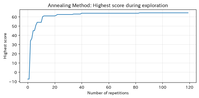

Reading the results

Even if you start from the current conditions, temporarily accepting the deterioration plan allows you to move into another promising area. However, since it is a single path, multiple executions with different starting points are the basic practice in practice.

No.085: Bayesian Optimization

Meaning in Practice

When a single high-precision simulation takes several hours, Bayesian optimization is effective in finding promising conditions with fewer evaluations.

Approach to Analysis and Modeling

From the evaluated points, the average score $\mu(x)$ and uncertainty $\sigma(x)$ during the Gaussian process are estimated, and the points with the higher Expected Improvement (EI) are then evaluated. We balance utilizing known high-quality areas with exploring unknown areas.

Check with Python

rng = np.random.default_rng(8500)
pool = np.array([(w,b,p) for w in range(3,8) for b in range(10,81,5) for p in range(15,76,5)])
chosen = list(rng.choice(len(pool), 8, replace=False))
y = [business_score(evaluate_policy(*pool[i], n_days=180, seed=85000+k)) for k,i in enumerate(chosen)]
bo_best = [max(y)]
for t in range(12):
    X = pool[chosen] / np.array([7, 80, 75])
    gp = GaussianProcessRegressor(kernel=Matern(nu=2.5)+WhiteKernel(.5), normalize_y=True,
                                  random_state=BASE_SEED).fit(X, y)
    available = np.array([i for i in range(len(pool)) if i not in chosen])
    mu, sd = gp.predict(pool[available] / np.array([7,80,75]), return_std=True)
    z = (mu - max(y)) / np.maximum(sd, 1e-9)
    ei = (mu-max(y))*norm.cdf(z) + sd*norm.pdf(z)
    idx = available[np.argmax(ei)]
    chosen.append(idx)
    y.append(business_score(evaluate_policy(*pool[idx], n_days=180, seed=85100+t)))
    bo_best.append(max(y))
bo_gene = pool[chosen[int(np.argmax(y))]]
pd.DataFrame([evaluate_policy(*bo_gene, n_days=1000, seed=85999)]).round(2)

	workers	buffer	pm_interval	mean_profit	p05_profit	on_time_rate	mean_wip	downtime_h
0	6	30	45	62.94	26.88	0.91	5.52	0.1

plt.figure(figsize=(7, 3.5))
plt.plot(range(len(bo_best)), bo_best, marker="o")
plt.title("Bayesian Optimization: Highest score through additional evaluation")
plt.xlabel("Number of additional evaluations")
plt.ylabel("Highest score")
plt.grid(True, alpha=.3)
plt.tight_layout()
plt.show()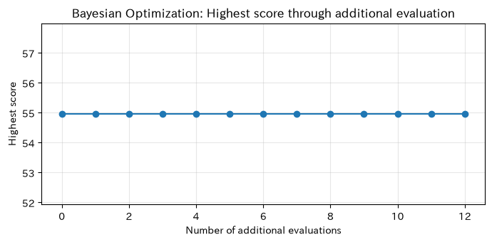

Reading the results

Not all candidates are evaluated; only the points chosen by proxy models are additionally evaluated. It can also leave runner-up candidates and prediction uncertainties, making it useful for prioritizing additional verification.

No.086: Introduction to Optuna

Meaning in Practice

With Optuna, trial numbers, parameters, and target values can be consistently saved, reducing manual omissions caused by personnel during searches.

Approach to Analysis and Modeling

Propose candidates within the objective function and return the simulation results. In production, we design persistence to RDB, multiple workers, and trial shutdown conditions.

Check with Python

import optuna
optuna.logging.set_verbosity(optuna.logging.WARNING)

def objective(trial):
    w = trial.suggest_int("workers", 3, 7)
    b = trial.suggest_int("buffer", 10, 80, step=5)
    pm = trial.suggest_int("pm_interval", 15, 75, step=5)
    r = evaluate_policy(w, b, pm, n_days=180, seed=86000 + trial.number)
    return business_score(r)

study = optuna.create_study(direction="maximize", sampler=optuna.samplers.TPESampler(seed=8600))
study.optimize(objective, n_trials=35)
optuna_best = [study.best_params[k] for k in ["workers", "buffer", "pm_interval"]]
pd.DataFrame([{**study.best_params, "best_score": study.best_value}]).round(2)

	workers	buffer	pm_interval	best_score
0	5	75	55	66.18

trials = study.trials_dataframe()
plt.figure(figsize=(7, 3.5))
plt.scatter(trials["number"], trials["value"], alpha=.65, label="Each trial implementation")
plt.plot(trials["number"], trials["value"].cummax(), color="red", label="Cumulative Highest")
plt.title("OptunaSearch history")
plt.xlabel("trial number")
plt.ylabel("Score")
plt.grid(True, alpha=.3)
plt.legend()
plt.tight_layout()
plt.show()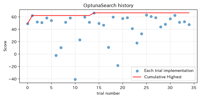

Reading the results

You can check for improvement plateaus and outliers from the trial history. Recording not only search results but also code, random number seeds, and input number counts as a set leads to reproducibility.

No.087: Mathematical Optimization × Simulation

Meaning in Practice

Simulation excels at uncertain capability assessments, while mathematical optimization excels at determining allocations under explicit resource constraints. By dividing the responsibilities between the two, you can even handle allocating improvement budgets across multiple lines.

Approach to Analysis and Modeling

The effects of each line and improvement plan are estimated through simulation, and the expected profit increase is passed to the 0-1 integer plan as a coefficient.

$\max \sum_i v_i z_i\quad \text{s.t.}\quad \sum_i c_i z_i\leq B,\; z_i\in\{0,1\}$

Check with Python

projects = pd.DataFrame({
    "project": ["ALine Increase", "Aline buffer", "BLine Preventive Maintenance", "BLine Increase", "Inspection automation"],
    "cost": [55, 28, 36, 50, 68],
    "annual_value": [74, 31, 49, 61, 82],
})
budget = 120
res = milp(c=-projects["annual_value"].to_numpy(), integrality=np.ones(len(projects)),
           bounds=Bounds(np.zeros(len(projects)), np.ones(len(projects))),
           constraints=LinearConstraint(projects["cost"].to_numpy()[None, :], -np.inf, budget))
projects["selected"] = np.rint(res.x).astype(int)
projects

	project	cost	annual_value	selected
0	ALine Increase	55	74	1
1	Aline buffer	28	31	1
2	BLine Preventive Maintenance	36	49	1
3	BLine Increase	50	61	0
4	Inspection automation	68	82	0

selected = projects.query("selected == 1")
print("budget for use:", selected["cost"].sum(), "/", budget)
print("Expected Annual Value:", selected["annual_value"].sum())

Budget: 119 / 120
Expected annual value: 154

Reading the results

Rather than simply ranking by cost-effectiveness, the combination that maximizes total value within the budget is chosen. Since there is an error in the simulation coefficients themselves, cases at the selection boundary require sensitivity analysis that adjusts the coefficients up or down.

No.088: Integration with Reinforcement Learning

Meaning in Practice

If you need state-dependent rules such as “call for support on days with many stagnations” rather than fixed optimal conditions, reinforcement learning (RL) becomes a candidate.

Approach to Analysis and Modeling

In a simplified daily environment, status is classified as low, medium, or high retention; actions are ‘no support’ or ‘1 person’ or ‘2 people’; and compensation is calculated by subtracting labor and retention costs from processing value. Q: We update long-term rewards through learning.

Check with Python

rng = np.random.default_rng(8800)
Q = np.zeros((3, 3))
alpha, gamma, epsilon = .12, .92, .18
for episode in range(600):
    backlog = int(rng.integers(0, 25))
    for day in range(50):
        state = min(backlog // 18, 2)
        action = rng.integers(3) if rng.random() < epsilon else int(np.argmax(Q[state]))
        demand = max(70, rng.normal(112, 18))
        capacity = 104 + 10 * action + rng.normal(0, 5)
        processed = min(backlog + demand, capacity)
        backlog = max(0, int(backlog + demand - processed))
        reward = 1.5 * processed - 13 * action - .35 * backlog
        next_state = min(backlog // 18, 2)
        Q[state, action] += alpha * (reward + gamma * Q[next_state].max() - Q[state, action])
policy = pd.DataFrame(Q.round(1), index=["detention:low", "detention:middle", "detention:high"],
                      columns=["Support0name", "Support1name", "Support2name"])
policy["Selective behavior"] = [f"Support{a}name" for a in np.argmax(Q, axis=1)]
policy

	Support0name	Support1name	Support2name	Selective behavior
detention:low	1842.6	1825.0	1828.1	Support0name
detention:middle	1828.7	1827.5	1840.8	Support2name
detention:high	1789.2	1812.2	1839.6	Support2name

fig, ax = plt.subplots(figsize=(6.5, 3.5))
im = ax.imshow(Q, cmap="Blues", aspect="auto")
ax.set_xticks(range(3), ["0name", "1name", "2name"])
ax.set_yticks(range(3), ["low", "middle", "high"])
ax.set_title("Post-learning state and behavioral value (QValue)")
ax.set_xlabel("Number of supporters")
ax.set_ylabel("stagnant state")
ax.grid(False)
fig.colorbar(im, ax=ax, label="Qvalue")
plt.tight_layout()
plt.show()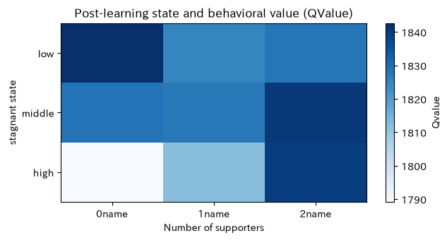

Reading the results

The number of supporters selected changes for each stagnant state, and operational rules differ from fixed placements. However, without directly connecting to the actual equipment, offline evaluation, action limits, manual intervention, and default actions in case of abnormalities are predetermined first.

No.089: Digital Twin

Meaning in Practice

Digital twins are not 3D displays themselves; rather, they update status and parameters based on field performance, estimate the future, and return them to decision-making in a cycle.

Approach to Analysis and Modeling

Without fixing the probability of failure, the beta distribution parameters are updated daily based on whether the system is stopped or not. If you observe a failure $f$ a failure $Beta(a,b)$ and a non-fault $n$, the post-distribution is $Beta(a+f,b+n)$.

Check with Python

rng = np.random.default_rng(8900)
true_prob = np.r_[np.repeat(.045, 60), np.repeat(.11, 60)]
observed = rng.random(120) < true_prob
a, b = 2., 38.
posterior_mean = []
for failed in observed:
    a += failed
    b += 1 - failed
    posterior_mean.append(a / (a + b))
twin = pd.DataFrame({"day": np.arange(1,121), "actual_failure_prob": true_prob,
                     "posterior_mean": posterior_mean, "failed": observed})
twin.tail().round(3)

	day	actual_failure_prob	posterior_mean	failed
115	116	0.11	0.064	False
116	117	0.11	0.064	False
117	118	0.11	0.070	True
118	119	0.11	0.069	False
119	120	0.11	0.069	False

plt.figure(figsize=(8, 3.6))
plt.plot(twin["day"], twin["actual_failure_prob"], linestyle="--", label="True Probability of Failure (Fictional)")
plt.plot(twin["day"], twin["posterior_mean"], label="Twin Estimates")
plt.scatter(twin.loc[twin.failed, "day"], np.repeat(.145, twin.failed.sum()), marker="x", color="red", label="Fault Observation")
plt.title("Continuous updates of failure probability based on actual data")
plt.xlabel("days")
plt.ylabel("failure probability")
plt.grid(True, alpha=.3)
plt.legend()
plt.tight_layout()
plt.show()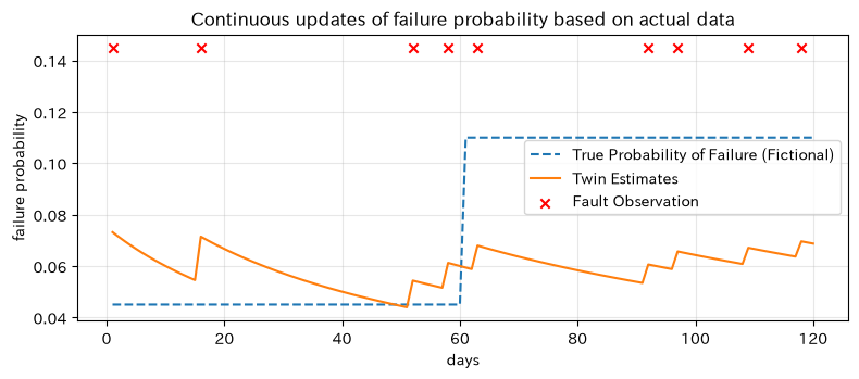

Reading the results

Deterioration after the 60th day will be monitored according to observations. If the follow-up is too slow, consider the forgetting factor or state-space model. If you don’t monitor for data delays, missing sensors, or mismatches in equipment IDs, you’ll end up with ‘plausible incorrect models’ that are updated.

No.090: What-if Analysis

Meaning in Practice

Management meetings require comparisons based on conditions, such as “if demand increases by 15%” or “if recovery from failures takes longer” rather than a single forecast. What-if analysis is a method of clarifying assumptions to confirm the resistance of alternatives.

Approach to Analysis and Modeling

The baseline proposal, top grid proposal, and Optuna proposal are evaluated under the same scenario: normal, increased demand, prolonged failures, and compound stress. The common random number makes it easier to compare differences between proposals.

Check with Python

grid_best = grid.loc[0, ["workers", "buffer", "pm_interval"]].astype(int).tolist()
plans = {"standard draft": [4,30,45], "Top grid proposals": grid_best, "Optunacase": optuna_best}
scenarios = {"usually": (112,1.0), "need15%increase": (129,1.0), "Prolonged recovery": (112,1.6), "Compound stress": (129,1.6)}
rows = []
for s, (dm, fs) in scenarios.items():
    for name, x in plans.items():
        r = evaluate_policy(*x, n_days=1200, seed=9000, demand_mean=dm, failure_scale=fs)
        rows.append({"scenario": s, "plan": name, **r})
whatif = pd.DataFrame(rows)
whatif[["scenario", "plan", "mean_profit", "p05_profit", "on_time_rate", "mean_wip"]].round(2)

	scenario	plan	mean_profit	p05_profit	on_time_rate	mean_wip
0	usually	standard draft	71.60	22.69	0.72	12.69
1	usually	Top grid proposals	61.70	25.70	0.94	4.93
2	usually	Optunacase	68.98	32.85	0.88	7.39
3	need15%increase	standard draft	56.93	-26.61	0.35	22.05
4	need15%increase	Top grid proposals	71.30	29.88	0.77	14.43
5	need15%increase	Optunacase	72.47	9.93	0.66	18.71
6	Prolonged recovery	standard draft	69.30	17.24	0.72	12.79
7	Prolonged recovery	Top grid proposals	60.56	24.45	0.94	5.10
8	Prolonged recovery	Optunacase	66.44	30.29	0.88	7.91
9	Compound stress	standard draft	54.44	-32.06	0.35	22.10
10	Compound stress	Top grid proposals	70.02	29.45	0.76	14.55
11	Compound stress	Optunacase	69.48	1.11	0.66	19.23

fig, axes = plt.subplots(1, 2, figsize=(11, 3.8))
for name in plans:
    d = whatif[whatif.plan == name]
    axes[0].plot(d.scenario, d.mean_profit, marker="o", label=name)
    axes[1].plot(d.scenario, d.on_time_rate, marker="o", label=name)
axes[0].set_title("Average profit by scenario")
axes[0].set_xlabel("Scenario")
axes[0].set_ylabel("Profit (ten thousand yen)/Day)")
axes[1].set_title("Delivery Rate by Scenario")
axes[1].set_xlabel("Scenario")
axes[1].set_ylabel("On-time delivery rate")
for ax in axes:
    ax.grid(True, alpha=.3)
    ax.tick_params(axis="x", rotation=20)
axes[1].axhline(.95, color="red", linestyle="--", label="Objective95%")
axes[1].legend()
plt.tight_layout()
plt.show()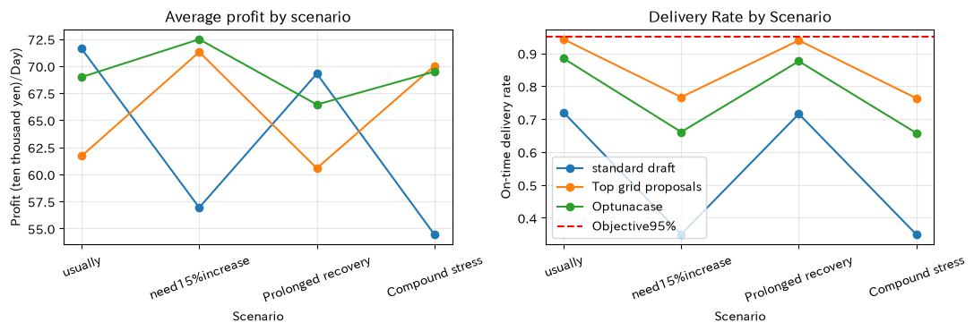

Reading the results

Even if the top plan under normal circumstances is under combined stress, it doesn’t necessarily mean it is number one; there are scenarios where the delivery target is exceeded. In management decisions, we present the “expected profit in the most frequent scenario,” “worst-case loss,” and “recovery measures” as a set. What-if is not a prediction of the future, but a tool that shares decision-making boundaries when assumptions change.

7. Practical Insights Seen Through Target Exercise

1. Agreement on the objective function comes first: Prioritize profit, delivery time, WIP, and safety before algorithms.
2. Separating exploration from verification: High scores during exploration will be re-evaluated under long-term, different, and stress conditions.
3. Choose methods based on computational cost and variable structure: If there are few candidates, grid is the option; for discrete combinations, GA/SA is the option; for expensive valuations, Bayesian optimization is a good choice.
4. Distinguishing between fixed conditions and dynamic measures: Optimize capital investment, align daily support decisions with RL, and align the timeline for decision-making.
5. Turning Models into Assets Under Management: Only when there is a person responsible for performance updates, version management, monitoring, and recalculation can it become a digital twin.

8. What is necessary for practical implementation

• A decision definition document stating objectives, KPIs, constraints, approvers, and usage frequency
• Master maintenance and time synchronization of products, equipment, processes, and stoppage reasons
• Validation verification by performance period, expert review, sensitivity analysis
• Version management of input data, code, dependencies, random number seeds, and execution results
• On-site behavioral constraints, fallback in case of abnormalities, manual overwriting
• Operational design to monitor KPI differences, model degradation, and data shortages after implementation

Optimization results are not just instructions, but decisions made with assumptions and risks. Safety and quality constraints will not be replaced by profit penalties; instead, they will be hard constraints that define feasibility in principle.

9. Summary

From No.081 to No.090, we connected the simulation objective design, exploration, resource allocation, dynamic control, performance updates, and scenario comparison through a single fictional line. The practical value lies not in “producing a single optimal value,” but in creating a decision-making process where multiple departments compare proposals based on the same assumptions and recalculate when conditions change.

10. Consultations for Corporations

At Surikoubo, we support everything from simulation design and mathematical optimization for manufacturing industries, to demand and failure uncertainty assessment, and from PoC to operational infrastructure development. Even if the issue is not yet formulated, you can consult us about decision-making and data organization.

📩 Contact Us: surikobo.co.jp/contact
Please feel free to consult us first.