Discrete event simulation to prevent disruption of the variant factory flow

No.041–No.050: Recreating the Process from Order Receipt to Completion in a Virtual Factory

This article covers a fictional precision parts factory as a subject, covering everything from the basic structure of Discrete Event Simulation (DES） to production lines, processes, job shops, and flow shops. The effects of “waiting,” “competition,” and “order,” which are easy to overlook with average processing time alone, are visualized with executable Python code and converted into criteria for decision-making decisions on delivery dates, work-in-progress, and capital investment.

[!NOTE] This material is a notebook previously used by Surikoubo (or personally by the representative, Kazuyama), and has been reconstructed, edited, and published with the company’s permission.
All data listed is fictional and has no relation whatsoever to real companies, factories, or figures.

Introduction: Practical Challenges in Manufacturing Covered in This Article

The target factory produces multiple types of metal parts to order, which are then machined, ground, and inspected before shipping. While equipment utilization rates are high on site, delays in delivery and work-in-progress are increasing. The question in this article is: Where to add your abilities, and in what order to streamline work to stabilize deadlines..

In DES, time only advances at the moment the condition changes, such as order arrival, processing start, processing completion, or failure. This allows you to reproduce real-world competition and waiting without having to calculate all equipment in seconds.

Common situations on site

• On a monthly average, there is enough capacity, but it only lingers during specific time periods.
• As a result of increasing uptime, both work-in-progress and lead times increase.
• The process sequence differs by product type, making it impossible to track equipment competition with just spreadsheets.
• They want to try equipment expansion plans, but testing them on the actual line is costly.

Why is this issue so difficult to judge?

This is because variations in processing times, simultaneous arrivals, exclusive use of equipment, and priorities interact with each other. Static capability calculations made only by averages cannot express “when it will be crowded” or “who will wait.” DES models this time dependence. However, if the input distribution or operational rules are inaccurate, the results will also be inaccurate, so sensitivity analysis and on-site verification are essential.

Overview of Exercise covered this time

No.	Theme	Perspectives gained from practical work
041	What is DES?	A model that only tracks state changes
042	Event List	Explainability through time-series logs
043	Future Event List	Managing the Next Events
044	Event Scheduling Methods	Event-Centric Implementation
045	Process Interaction Law	Implementation centered on product flow
046	SimPy Introduction	Simply expressing resource competition
047	Production Line	Comparing the What-If of Ability Changes
048	Process Simulation	Diagnosis of Retention and Utilization Rates
049	job shop	Competition by Variety Route
050	Flow Shop	Insertion order and makeup

Preparing the Python environment

The random number generator is fixed for reproducibility. Below, we use only numpy, pandas, matplotlib, and simpy without using external data.

import sys
import numpy as np
import pandas as pd
import matplotlib
import matplotlib.pyplot as plt
import simpy
from IPython.display import display

SEED = 42
np.random.seed(SEED)
pd.set_option("display.max_columns", 20)
print(f"Python {sys.version.split()[0]}")
print(f"numpy {np.__version__}, pandas {pd.__version__}, matplotlib {matplotlib.__version__}, simpy {simpy.__version__}")

Python 3.13.1
numpy 2.5.1, pandas 3.0.3, matplotlib 3.11.0, simpy 4.1.2

Creation of Fictional Data

For the three varieties, we generate standard processing times for each process and one day’s worth of orders. The unit is minutes. Arrival intervals and processing times are actually estimated distributions from actual data, but here we use known distributions for explanation.

rng = np.random.default_rng(SEED)
routing = pd.DataFrame({
    "product": ["A", "B", "C"],
    "route": [["Cut", "Grind", "Inspect"], ["Cut", "Inspect"], ["Grind", "Cut", "Inspect"]],
    "Cut": [18, 24, 15], "Grind": [14, 0, 22], "Inspect": [8, 10, 12]
})
arrival = np.cumsum(rng.exponential(18, size=24))
orders = pd.DataFrame({
    "job": [f"J{i:02d}" for i in range(1, 25)],
    "product": rng.choice(["A", "B", "C"], 24, p=[0.45, 0.35, 0.20]),
    "arrival": arrival.round(1),
    "due": (arrival + rng.integers(90, 181, 24)).round(1),
})
display(routing)
display(orders.head(8))

	product	route	Cut	Grind	Inspect
0	A	[Cut, Grind, Inspect]	18	14	8
1	B	[Cut, Inspect]	24	0	10
2	C	[Grind, Cut, Inspect]	15	22	12

	job	product	arrival	due
0	J01	B	43.3	154.3
1	J02	A	85.3	237.3
2	J03	B	128.3	275.3
3	J04	A	133.3	235.3
4	J05	A	134.8	299.8
5	J06	B	161.0	269.0
6	J07	B	186.4	349.4
7	J08	C	242.6	332.6

No.041: What is DES?

Meaning in Practice

By tracking only the points when equipment or product conditions change, you can reproduce wait times and changes in work-in-progress with reduced computational workload. This serves as the foundation for virtual experiments that change equipment capacity, deployment intervals, and operational rules.

Approach to Analysis and Modeling

If you set the system state to $S(t)$ and the event time to $t_k$, the state remains constant between events and updates to $S(t_k^+)=f(S(t_k^-), e_k)$. Here, we check the arrival of three jobs per unit using the smallest manually calculated model.

Check with Python

jobs = pd.DataFrame({"job": ["J1", "J2", "J3"], "arrival": [0, 4, 9], "process": [7, 5, 6]})
available = 0
rows = []
for r in jobs.itertuples():
    start = max(r.arrival, available); finish = start + r.process
    rows.append([r.job, r.arrival, start, finish, start-r.arrival])
    available = finish
des_basic = pd.DataFrame(rows, columns=["job", "arrival", "start", "finish", "wait"])
display(des_basic)

	job	arrival	start	finish	wait
0	J1	0	0	7	0
1	J2	4	7	12	3
2	J3	9	12	18	3

Reading the results

At J2, you have to wait 3 minutes until the 7 minutes when the facilities become available. You can see that not only the average processing time but also the timing of arrival and equipment release determines the waiting time.

No.042: Event List

Meaning in Practice

The event log is an audit trail that explains at which process and time the delivery delay occurred. It can also be used for on-site interviews and matching with performance logs.

Approach to Analysis and Modeling

Events should have at least a minimum time, target, type, and state changes. By pairing start and end records, you can later re-aggregate equipment occupancy time, waiting times, and work-in-progress trends.

Check with Python

event_log = []
for r in des_basic.itertuples():
    event_log += [(r.arrival, r.job, "ARRIVAL"), (r.start, r.job, "START"), (r.finish, r.job, "FINISH")]
event_log = pd.DataFrame(event_log, columns=["time", "job", "event"]).sort_values(["time", "event"]).reset_index(drop=True)
display(event_log)

	time	job	event
0	0	J1	ARRIVAL
1	0	J1	START
2	4	J2	ARRIVAL
3	7	J1	FINISH
4	7	J2	START
5	9	J3	ARRIVAL
6	12	J2	FINISH
7	12	J3	START
8	18	J3	FINISH

Reading the results

By logging by chronological order, you can reproduce the fact that you waited for equipment from the arrival of J2 until it started. In production, leaving the reason code and equipment ID makes it easier to use in improvement meetings.

No.043：Future Event List

Meaning in Practice

The Future Event List (FEL) is at the core of DES, managing the next events in chronological order. You can handle different events such as breakdowns and setup completions on a single timeline.

Approach to Analysis and Modeling

FEL is implemented as a priority queue. Extract the event with the minimum time, update the state, and repeat the process of adding necessary future events. The priority of simultaneous events is explicitly stated to affect the results.

Check with Python

import heapq
fel = [(0, 1, "J1", "ARRIVAL"), (4, 2, "J2", "ARRIVAL"), (9, 3, "J3", "ARRIVAL")]
heapq.heapify(fel); fel_trace = []
while fel:
    time, seq, job, event = heapq.heappop(fel)
    fel_trace.append((time, job, event, len(fel)))
    if event == "ARRIVAL":
        p = int(jobs.loc[jobs.job.eq(job), "process"].iloc[0])
        heapq.heappush(fel, (time + p, seq + 100, job, "PLANNED_FINISH"))
display(pd.DataFrame(fel_trace, columns=["time", "job", "event", "events_remaining_after_pop"]))

	time	job	event	events_remaining_after_pop
0	0	J1	ARRIVAL	2
1	4	J2	ARRIVAL	2
2	7	J1	PLANNED_FINISH	2
3	9	J3	ARRIVAL	1
4	9	J2	PLANNED_FINISH	1
5	15	J3	PLANNED_FINISH	0

Reading the results

FEL always takes the minimum time. This simplified example does not yet address equipment conflicts, but it clearly explains how events are added and time progression works.

No.044: Event Scheduling Method

Meaning in Practice

It is suitable for strictly controlling equipment-centric logic or complex event rules. Implementers specify state transitions for each event.

Approach to Analysis and Modeling

In event scheduling, you consider functions that handle “arrival” and “completion,” and start the next job from the queue upon completion. The main KPIs are average wait time, maximum waiting time, and end time.

Check with Python

def event_scheduling(jobs_df):
    waiting, busy, seq, out, q = [], False, 0, {}, []
    for r in jobs_df.itertuples(): heapq.heappush(q, (r.arrival, seq, "ARRIVAL", r.job, r.process)); seq += 1
    while q:
        t, _, ev, job, p = heapq.heappop(q)
        if ev == "ARRIVAL": waiting.append((job, p, t))
        else: busy = False; out[job]["finish"] = t
        if not busy and waiting:
            j, pt, a = waiting.pop(0); busy = True
            out[j] = {"start": t, "wait": t-a}; heapq.heappush(q, (t+pt, seq, "FINISH", j, pt)); seq += 1
    return pd.DataFrame(out).T.reset_index(names="job")
event_result = event_scheduling(jobs)
display(event_result)

	job	start	wait	finish
0	J1	0	0	7
1	J2	7	3	12
2	J3	12	3	18

Reading the results

The result of clearly stating the event rules matches the calculation in No.041. As rules increase, state management becomes more complex, so it is important to break them down into small, testable event functions.

No.045: Process Interaction Method

Meaning in Practice

It is a method that allows you to describe the process of products and workers moving sequentially through each process, making it easy to confirm the correspondence between process designers and models.

Approach to Analysis and Modeling

Each job is represented as an independent process, requiring the necessary equipment, waiting until it is secured, and then releasing it after processing. Internally, it is event processing, but the code is closer to business workflows.

Check with Python

def process_interaction(jobs_df):
    env = simpy.Environment(); machine = simpy.Resource(env, capacity=1); rec = []
    def job_proc(row):
        yield env.timeout(row.arrival)
        with machine.request() as req:
            yield req; start = env.now; yield env.timeout(row.process)
            rec.append((row.job, row.arrival, start, env.now, start-row.arrival))
    for row in jobs_df.itertuples(): env.process(job_proc(row))
    env.run(); return pd.DataFrame(rec, columns=["job", "arrival", "start", "finish", "wait"])
process_result = process_interaction(jobs)
display(process_result.sort_values("job"))

	job	arrival	start	finish	wait
0	J1	0	0	7	0
1	J2	4	7	12	3
2	J3	9	12	18	3

Reading the results

We were able to briefly express waiting for the same equipment as a job action. When the process route is long, it has the advantage of making it easier to match the model with the standard work sheet.

No.046: Introduction to SimPy

Meaning in Practice

Using SimPy’s Resources, you can represent finite resources such as the number of equipment, workers, and inspection tables. You can compare additional equipment proposals with just one code change.

Approach to Analysis and Modeling

Environment represents the time, Resource represents the exclusive resource, and timeout represents the required time. Compare Abilities 1 and 2 to check their effect on the wait time.

Check with Python

simpy_compare = []
for capacity in [1, 2]:
    env = simpy.Environment(); machine = simpy.Resource(env, capacity=capacity); waits = []
    def part(env, arrival, duration):
        yield env.timeout(arrival)
        with machine.request() as req:
            yield req; waits.append(env.now-arrival); yield env.timeout(duration)
    for r in jobs.itertuples(): env.process(part(env, r.arrival, r.process))
    env.run(); simpy_compare.append((capacity, np.mean(waits), max(waits)))
display(pd.DataFrame(simpy_compare, columns=["capacity", "mean_wait", "max_wait"]))

	capacity	mean_wait	max_wait
0	1	2.0	3
1	2	0.0	0

Reading the results

In this small-scale example, having two units eliminates the wait. However, in practice, since there is a possibility of stagnation shifting to subsequent processes, evaluation is conducted across the entire line.

No.047: Production Line Simulation

Meaning in Practice

On series lines, improving a single process does not necessarily lead to an increase in the number of completed products. Simultaneous resource competition for cutting, grinding, and inspection, and comparing equipment enhancement plans.

Approach to Analysis and Modeling

The lead time for Job $j$ is $L_j=C_j-A_j$, and the delivery delay is $T_j=\max(0,C_j-D_j)$. Not only the number of completed items but also the average lead time and on-time delivery rate are also listed.

Check with Python

def simulate_factory(capacity=None, horizon=600, seed=SEED):
    capacity = capacity or {"Cut": 1, "Grind": 1, "Inspect": 1}
    env = simpy.Environment(); rng_local = np.random.default_rng(seed)
    machines = {m: simpy.Resource(env, capacity=capacity[m]) for m in capacity}
    records, operations = [], []
    route_map = routing.set_index("product").to_dict("index")
    def job_proc(row):
        yield env.timeout(row.arrival)
        for machine in route_map[row.product]["route"]:
            queued = env.now
            with machines[machine].request() as req:
                yield req; start = env.now
                mean = route_map[row.product][machine]
                duration = max(1, rng_local.normal(mean, mean*0.15))
                yield env.timeout(duration)
                operations.append((row.job, row.product, machine, queued, start, env.now))
        records.append((row.job, row.product, row.arrival, env.now, row.due))
    for row in orders.itertuples(): env.process(job_proc(row))
    env.run(until=horizon)
    res = pd.DataFrame(records, columns=["job", "product", "arrival", "finish", "due"])
    if len(res):
        res["lead_time"] = res.finish-res.arrival; res["tardiness"] = (res.finish-res.due).clip(lower=0)
    ops = pd.DataFrame(operations, columns=["job", "product", "machine", "queued", "start", "finish"])
    return res, ops

scenarios = {"Current Status": {"Cut":1,"Grind":1,"Inspect":1}, "cutting2platform": {"Cut":2,"Grind":1,"Inspect":1}, "grinding2platform": {"Cut":1,"Grind":2,"Inspect":1}}
summary=[]
for name, cap in scenarios.items():
    r, _ = simulate_factory(cap)
    summary.append((name, len(r), r.lead_time.mean(), (r.tardiness==0).mean()))
line_summary=pd.DataFrame(summary, columns=["scenario","completed","mean_lead_time","on_time_rate"])
display(line_summary.round(2))
line_summary.set_index("scenario")[["mean_lead_time"]].plot(kind="bar", color="#2878B5", legend=False)
plt.title("Capacity scenario and mean lead time"); plt.xlabel("Scenario"); plt.ylabel("Mean lead time [min]"); plt.grid(axis="y", alpha=.3); plt.tight_layout(); plt.show()

	scenario	completed	mean_lead_time	on_time_rate
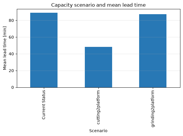
0	Current Status	24	89.00	0.67
1	cutting2platform	24	48.36	1.00
2	grinding2platform	23	87.20	0.78

/var/folders/3y/fmw40k0x78xblvb3gkcyvy1h0000gn/T/ipykernel_20161/4039603803.py:34: UserWarning: Glyph 29694 (\N{CJK UNIFIED IDEOGRAPH-73FE}) missing from font(s) DejaVu Sans.
  plt.title("Capacity scenario and mean lead time"); plt.xlabel("Scenario"); plt.ylabel("Mean lead time [min]"); plt.grid(axis="y", alpha=.3); plt.tight_layout(); plt.show()
/var/folders/3y/fmw40k0x78xblvb3gkcyvy1h0000gn/T/ipykernel_20161/4039603803.py:34: UserWarning: Glyph 29366 (\N{CJK UNIFIED IDEOGRAPH-72B6}) missing from font(s) DejaVu Sans.
  plt.title("Capacity scenario and mean lead time"); plt.xlabel("Scenario"); plt.ylabel("Mean lead time [min]"); plt.grid(axis="y", alpha=.3); plt.tight_layout(); plt.show()
/var/folders/3y/fmw40k0x78xblvb3gkcyvy1h0000gn/T/ipykernel_20161/4039603803.py:34: UserWarning: Glyph 20999 (\N{CJK UNIFIED IDEOGRAPH-5207}) missing from font(s) DejaVu Sans.
  plt.title("Capacity scenario and mean lead time"); plt.xlabel("Scenario"); plt.ylabel("Mean lead time [min]"); plt.grid(axis="y", alpha=.3); plt.tight_layout(); plt.show()
/var/folders/3y/fmw40k0x78xblvb3gkcyvy1h0000gn/T/ipykernel_20161/4039603803.py:34: UserWarning: Glyph 21066 (\N{CJK UNIFIED IDEOGRAPH-524A}) missing from font(s) DejaVu Sans.
  plt.title("Capacity scenario and mean lead time"); plt.xlabel("Scenario"); plt.ylabel("Mean lead time [min]"); plt.grid(axis="y", alpha=.3); plt.tight_layout(); plt.show()
/var/folders/3y/fmw40k0x78xblvb3gkcyvy1h0000gn/T/ipykernel_20161/4039603803.py:34: UserWarning: Glyph 21488 (\N{CJK UNIFIED IDEOGRAPH-53F0}) missing from font(s) DejaVu Sans.
  plt.title("Capacity scenario and mean lead time"); plt.xlabel("Scenario"); plt.ylabel("Mean lead time [min]"); plt.grid(axis="y", alpha=.3); plt.tight_layout(); plt.show()
/var/folders/3y/fmw40k0x78xblvb3gkcyvy1h0000gn/T/ipykernel_20161/4039603803.py:34: UserWarning: Glyph 30740 (\N{CJK UNIFIED IDEOGRAPH-7814}) missing from font(s) DejaVu Sans.
  plt.title("Capacity scenario and mean lead time"); plt.xlabel("Scenario"); plt.ylabel("Mean lead time [min]"); plt.grid(axis="y", alpha=.3); plt.tight_layout(); plt.show()
/Users/hiroshi/private/kobo/notebook/.venv/lib/python3.13/site-packages/IPython/core/pylabtools.py:170: UserWarning: Glyph 29694 (\N{CJK UNIFIED IDEOGRAPH-73FE}) missing from font(s) DejaVu Sans.
  fig.canvas.print_figure(bytes_io, **kw)
/Users/hiroshi/private/kobo/notebook/.venv/lib/python3.13/site-packages/IPython/core/pylabtools.py:170: UserWarning: Glyph 29366 (\N{CJK UNIFIED IDEOGRAPH-72B6}) missing from font(s) DejaVu Sans.
  fig.canvas.print_figure(bytes_io, **kw)
/Users/hiroshi/private/kobo/notebook/.venv/lib/python3.13/site-packages/IPython/core/pylabtools.py:170: UserWarning: Glyph 20999 (\N{CJK UNIFIED IDEOGRAPH-5207}) missing from font(s) DejaVu Sans.
  fig.canvas.print_figure(bytes_io, **kw)
/Users/hiroshi/private/kobo/notebook/.venv/lib/python3.13/site-packages/IPython/core/pylabtools.py:170: UserWarning: Glyph 21066 (\N{CJK UNIFIED IDEOGRAPH-524A}) missing from font(s) DejaVu Sans.
  fig.canvas.print_figure(bytes_io, **kw)
/Users/hiroshi/private/kobo/notebook/.venv/lib/python3.13/site-packages/IPython/core/pylabtools.py:170: UserWarning: Glyph 21488 (\N{CJK UNIFIED IDEOGRAPH-53F0}) missing from font(s) DejaVu Sans.
  fig.canvas.print_figure(bytes_io, **kw)
/Users/hiroshi/private/kobo/notebook/.venv/lib/python3.13/site-packages/IPython/core/pylabtools.py:170: UserWarning: Glyph 30740 (\N{CJK UNIFIED IDEOGRAPH-7814}) missing from font(s) DejaVu Sans.
  fig.canvas.print_figure(bytes_io, **kw)

Reading the results

The effectiveness of equipment additions is assessed by combining the number of completed items, lead time, and on-time delivery rate. Expansion plans with little effect may not be the true constraint process. By adding the investment amount, you can expand the comparison to the cost per minute shortened or the amount of delay reduction.

No.048: Process Simulation

Meaning in Practice

By breaking down wait times and operating rates by process, you can link the locations where work-in-progress accumulates to the equipment load. Rather than simply aiming for high utilization rates, we look at the balance with delivery deadlines.

Approach to Analysis and Modeling

The operating rate for the $H$ observation period of the facility $m$ is $U_m=\sum p_{jm}/(c_mH)$. In high-load areas where wait times spike, small fluctuations can lead to significant congestion.

Check with Python

base_res, base_ops = simulate_factory(scenarios["Current Status"])
base_ops["wait"] = base_ops.start-base_ops.queued
process_kpi = base_ops.groupby("machine").agg(operations=("job","size"), mean_wait=("wait","mean"), busy_time=("finish", lambda s: 0.0))
busy = (base_ops.finish-base_ops.start).groupby(base_ops.machine).sum()
process_kpi["utilization"] = busy/600
display(process_kpi.round(3))
fig, ax = plt.subplots(figsize=(7,4)); process_kpi.mean_wait.plot(kind="bar", ax=ax, color="#F28E2B")
ax.set_title("Mean waiting time by process"); ax.set_xlabel("Process"); ax.set_ylabel("Mean wait [min]"); ax.grid(axis="y", alpha=.3); plt.tight_layout(); plt.show()

	operations	mean_wait	busy_time	utilization
machine
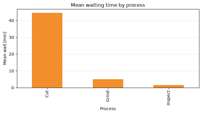
Cut	24	44.516	0.0	0.779
Grind	16	5.002	0.0	0.429
Inspect	24	1.526	0.0	0.377

Reading the results

Processes with long average wait times and high utilization rates are candidates for improvement. On the other hand, the average value hides some long waits, so in practice, 95th percentiles, time-in-progress by time, and reasons for stopping are also added.

No.049: Job Shop Simulation

Meaning in Practice

At job shops, the process sequence differs for each product type, and people compete for equipment. The choice of priority rules affects not only the average dwell time but also the bias in delivery delays.

Approach to Analysis and Modeling

Here, we check the results of three types passing through common equipment using Gantt charts. Strict rule comparisons involve repeatedly comparing FIFO, Shortest Processing Time (SPT), and Shortest Delivery Time (EDD) across the same random sequence.

Check with Python

sample_jobs = orders.job.iloc[:10]
gantt = base_ops[base_ops.job.isin(sample_jobs)].copy()
machine_y = {m:i for i,m in enumerate(["Cut","Grind","Inspect"])}
colors = {"A":"#4E79A7", "B":"#F28E2B", "C":"#59A14F"}
fig, ax = plt.subplots(figsize=(10,4.5))
for r in gantt.itertuples():
    ax.barh(machine_y[r.machine], r.finish-r.start, left=r.start, height=.55, color=colors[r.product], edgecolor="white")
    ax.text((r.start+r.finish)/2, machine_y[r.machine], r.job, ha="center", va="center", fontsize=7)
ax.set_yticks(list(machine_y.values()), list(machine_y.keys()))
ax.set_title("Job-shop schedule (first 10 jobs)"); ax.set_xlabel("Simulation time [min]"); ax.set_ylabel("Machine"); ax.grid(axis="x", alpha=.3); plt.tight_layout(); plt.show()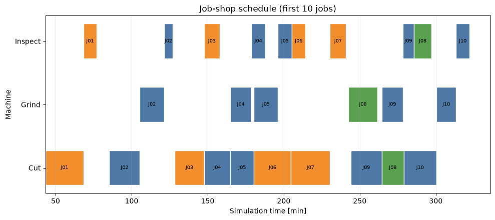

Reading the results

The Gantt chart shows a competition where Variety C progresses from grinding to cutting, while Variety A proceeds in reverse order. If orders are determined solely by local equipment efficiency, they may worsen the availability of other equipment or lead times, so rules are chosen based on KPIs covering all processes.

No.050: Flow Shop Simulation

Meaning in Practice

In flow shops where all products follow the same process sequence, the order of deployment affects the total completion time (makespan) and equipment idleness. If you need to change the setup, how you organize the variety is also important.

Approach to Analysis and Modeling

In the two-machine flow shop, the Johnson method is effective for minimizing makeup span. Short jobs from the first half of the machine are placed forward, and short jobs from the second half of the machine are placed backward. Here, we will check by comparing it with all permutations.

Check with Python

import itertools
flow = pd.DataFrame({"job":["P1","P2","P3","P4","P5"], "M1":[8,14,6,11,9], "M2":[12,7,15,9,10]}).set_index("job")
def makespan(seq):
    t1=t2=0
    for j in seq:
        t1 += flow.loc[j,"M1"]; t2 = max(t1,t2)+flow.loc[j,"M2"]
    return t2
best_seq = min(itertools.permutations(flow.index), key=makespan)
fifo_seq = tuple(flow.index)
comparison = pd.DataFrame({"sequence":[" → ".join(fifo_seq), " → ".join(best_seq)], "makespan":[makespan(fifo_seq), makespan(best_seq)]}, index=["FIFO","smallest"])
display(flow); display(comparison)
comparison.makespan.plot(kind="bar", color=["#9C9C9C","#59A14F"])
plt.title("Flow-shop sequencing comparison"); plt.xlabel("Rule"); plt.ylabel("Makespan [min]"); plt.grid(axis="y", alpha=.3); plt.tight_layout(); plt.show()

	M1	M2
job
P1	8	12
P2	14	7
P3	6	15
P4	11	9
P5	9	10

	sequence	makespan
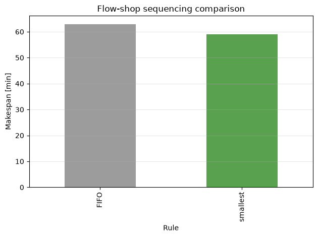
FIFO	P1 → P2 → P3 → P4 → P5	63
smallest	P3 → P1 → P2 → P4 → P5	59

/var/folders/3y/fmw40k0x78xblvb3gkcyvy1h0000gn/T/ipykernel_20161/4160123644.py:13: UserWarning: Glyph 26368 (\N{CJK UNIFIED IDEOGRAPH-6700}) missing from font(s) DejaVu Sans.
  plt.title("Flow-shop sequencing comparison"); plt.xlabel("Rule"); plt.ylabel("Makespan [min]"); plt.grid(axis="y", alpha=.3); plt.tight_layout(); plt.show()
/var/folders/3y/fmw40k0x78xblvb3gkcyvy1h0000gn/T/ipykernel_20161/4160123644.py:13: UserWarning: Glyph 23567 (\N{CJK UNIFIED IDEOGRAPH-5C0F}) missing from font(s) DejaVu Sans.
  plt.title("Flow-shop sequencing comparison"); plt.xlabel("Rule"); plt.ylabel("Makespan [min]"); plt.grid(axis="y", alpha=.3); plt.tight_layout(); plt.show()
/Users/hiroshi/private/kobo/notebook/.venv/lib/python3.13/site-packages/IPython/core/pylabtools.py:170: UserWarning: Glyph 26368 (\N{CJK UNIFIED IDEOGRAPH-6700}) missing from font(s) DejaVu Sans.
  fig.canvas.print_figure(bytes_io, **kw)
/Users/hiroshi/private/kobo/notebook/.venv/lib/python3.13/site-packages/IPython/core/pylabtools.py:170: UserWarning: Glyph 23567 (\N{CJK UNIFIED IDEOGRAPH-5C0F}) missing from font(s) DejaVu Sans.
  fig.canvas.print_figure(bytes_io, **kw)

Reading the results

Even with the same processing time, the makeup span changes just by the order of input. In practice, there are three or more processes, including delivery schedules, arrangements, and transport lots, so simulation and search algorithms are combined to verify the differences from the current order over several days.

Practical Implications Seen Through Target Exercise

1. Look at the timeline, not average ability: The concentration and variation of arrivals create waits.
2. Bottlenecks move: Upgrading equipment shifts constraints to later processes, so compare across the entire line.
3. Don’t just maximize utilization rates: High loads increase work-in-progress and delivery time variations.
4. Order with no additional investment for improvement: In job shops and flow shops, priority rules change KPIs.
5. Using logs for accountability: The event list allows you to track the reasons for the occurrence of simulation results.

What is necessary for practical implementation

• Define arrival times, processing, setup, stopping, and transport based on MES, PLC, and work performance
• Check for missing measurements, rounding, and mixing between planned and actual times, and estimate input distributions by type and equipment
• Confirm process routes, priority rules, breaks, and operations during breakdowns with on-site personnel
• Reproduce past periods and match the distribution of completed quantities, work-in-progress, and lead times with actual results.
• Generate confidence intervals with multiple seeds and iterations, and avoid using random single-trial attempts for decision-making.
• Creating a scenario evaluation table that includes investment costs, staffing constraints, and quality risks

A model is not a complete replica of reality, but a hypothesis of the resolution necessary for decision-making. Agreeing on the purpose, scope, tolerance of error, and renewal responsible party at the start is key to continued use.

Conclusion

From No.041 to No.050, we covered everything from DES event management, resource competition using SimPy, production line capability comparisons, process-specific KPIs, job shop visualization, and flow shop order comparison. The value of DES lies not in elaborate videos, but in Able to safely compare on-site operational plans and discuss delivery dates, work-in-progress, and investments on the same timeline..

Consultations for Corporations

At Suri Kobo, we support everything from organizing manufacturing performance data, bottleneck analysis, discrete event simulation, to what-if analysis of capital investment and personnel allocation, and building an analytical platform that can be continuously operated on-site. Even at stages where issues have not yet been quantified, we can work together from organizing target processes and decision-making.

📩 Contact Us: surikobo.co.jp/contact
Please feel free to consult us first.