Anticipating Changes in Production and Inventory: 10 Continuous Simulation Practices in Manufacturing

In this article, we use a fictional precision parts factory as the subject and capture How orders, production, inventory, and equipment status change over time through continuous simulation. Through No.061 to No.070, we verify everything from differential equation design, numerical calculations, demand and inventory feedback, to computational stability as a single decision story.

The goal is not to solve the equations themselves. It is important to be able to examine in reproducible ways such as “When will shortages be resolved if production increases?”, “Will ordering rules cause inventory fluctuations?”, and “Can calculation results be trusted as basis for meeting decisions”.

[!NOTE] This material is a notebook previously used by Surikoubo (or personally by the representative, Kazuyama), and has been reconstructed, edited, and published with the company’s permission.
All data listed is fictional and has no relation whatsoever to real companies, factories, or figures.

Introduction: Practical Challenges in Manufacturing Covered in This Article

The target factory has an assembly line that operates continuously in one-hour increments. Sales are anticipating increased demand, while manufacturing is considering capacity enhancement. On the other hand, increasing work-in-progress too much increases lead times and financial burdens, while over-reducing finished goods inventory leads to more shortages. Furthermore, equipment deterioration and delays in control rules can cause fluctuations not planned for the project.

Therefore, we model not only the “aggregated value at the current point” but also how states produce the next state. Continuous simulation is a method to compare changes in production ramp-up, maintenance cycles, and inventory standards—which are difficult to test with actual machines—as virtual experiments on a time axis.

Common situations on site

• Even if there is ample capacity on average per month, stockouts occur when demand rises.
• By checking inventory and adjusting production volumes, alternating between increased and decreased production
• Predictions a few days later can change just by the spreadsheet width or calculation formula
• Each department has different assumptions for “demand,” “capacity,” and “safety stock.”
• There are simulation results, but they do not lead to on-site KPIs or execution conditions.

Why is this issue so difficult to judge?

Manufacturing systems involve accumulation, lag, nonlinearity, and feedback. Inventory doesn’t reach the target value instantly; the gap between inflows and outflows accumulates over time. As equipment deterioration progresses, even the same specified quantity can lead to a decrease in actual production, and delays in judgment in response to demand changes can lead to overreaction. For this reason, simply comparing average values often overlooks transient shortages and oscillations.

Overview of Exercise covered this time

No.	Theme	Questions at the Factory	Key Indicators to Check
061	Differential equation model	How fast does the equipment condition change?	Temperature and equilibrium values
062	Euler method	How much results change over time	approximate error
063	Runge-Kutta method	How to balance accuracy and computational complexity	termination error
064	Lotka Volterra Model	Will competing resources cause cyclical fluctuations?	Work-in-progress and available capacity
065	SIR Model	How defective factors spread across processes.	Number of processes affected, peak time
066	System Dynamics	How to connect accumulation and flow to management metrics	Work-in-progress, throughput
067	Inventory Dynamics	Can increased production rules suppress shortages?	Inventory and out-of-stock times
068	Demand Dynamics	What does lagging behind demand shocks produce?	Demand, production instructions, and accumulated shortages
069	feedback loop	Does strong control stabilize inventory?	Overshoot, Finishing
070	Simulation stability	Whether numerical vibrations are mistaken for phenomena	Stability Conditions, Notch Width Sensitivity

The first half ensures the reliability of numerical calculations, and the second half expands to decision-making on inventory, demand, and control.

Preparing the Python environment

It does not rely on external data, using numpy, pandas, matplotlib, and scipy. The seed of the random number generator is fixed. japanize_matplotlib is used to display the Japanese of the graph.

%matplotlib inline
%config InlineBackend.figure_format = 'svg'

import platform
import numpy as np
import pandas as pd
import matplotlib
import matplotlib.pyplot as plt
import japanize_matplotlib
from scipy.integrate import solve_ivp

SEED = 20260712
rng = np.random.default_rng(SEED)
pd.set_option("display.float_format", "{:.3f}".format)

print("Python     :", platform.python_version())
print("numpy      :", np.__version__)
print("pandas     :", pd.__version__)
print("matplotlib :", matplotlib.__version__)
print("random seed:", SEED)

Python     : 3.11.9
numpy      : 1.26.4
pandas     : 2.2.2
matplotlib : 3.9.2
random seed: 20260712

Creation of Fictional Data

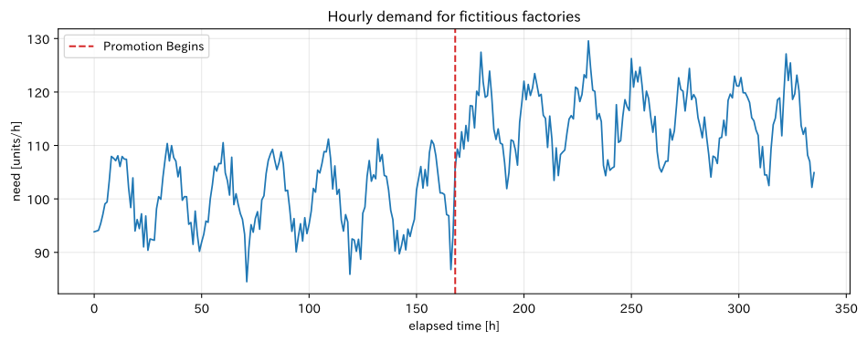
Demand is expected for 14 days (336 hours). The base demand is 100 units per hour, with daytime periodicity and increased promotions in the latter half of the week, resulting in small irregularities equivalent to forecast errors. All the values are fictional. From here on, this demand series and factory parameters will be used as common assumptions.

hours = np.arange(14 * 24)
daily_cycle = 8 * np.sin(2 * np.pi * (hours - 6) / 24)
promotion = np.where(hours >= 7 * 24, 15.0, 0.0)
noise = rng.normal(0, 2.5, len(hours))
demand = np.clip(100 + daily_cycle + promotion + noise, 80, None)

factory_data = pd.DataFrame({
    "time[h]": hours,
    "need[units/h]": demand,
    "Promotional Period": np.where(hours >= 7 * 24, "After the promotion", "usually"),
})
display(factory_data.head())
display(factory_data.groupby("Promotional Period")["need[units/h]"].agg(["mean", "std", "min", "max"]).round(2))

fig, ax = plt.subplots(figsize=(10, 4))
ax.plot(hours, demand, color="tab:blue", linewidth=1.3)
ax.axvline(7 * 24, color="tab:red", linestyle="--", label="Promotion Begins")
ax.set_title("Hourly demand for fictitious factories")
ax.set_xlabel("elapsed time [h]")
ax.set_ylabel("need [units/h]")
ax.grid(True, alpha=0.3)
ax.legend()
plt.tight_layout()
plt.show()

	time[h]	need[units/h]	Promotional Period
0	0	93.847	usually
1	1	93.977	usually
2	2	94.116	usually
3	3	95.370	usually
4	4	97.036	usually

	mean	std	min	max
Promotional Period
After the promotion	114.780	6.200	101.920	129.560
usually	99.960	6.270	84.510	111.230

No.061: Differential Equation Models

Meaning in Practice

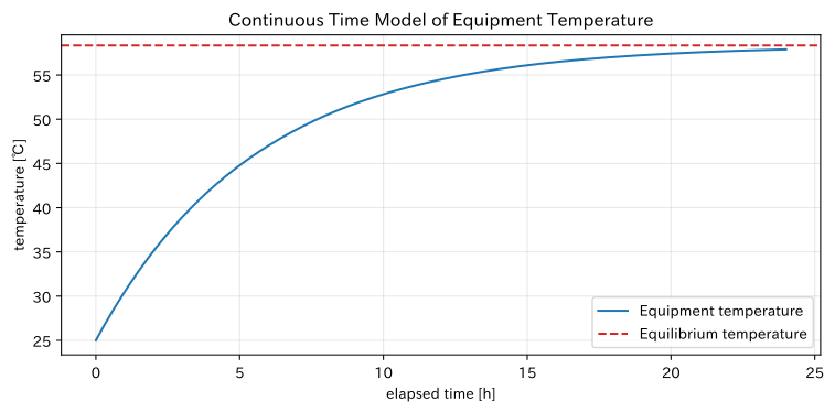
By managing equipment temperature, tank concentration, wear amount, work-in-progress volume, and other factors not only by current values but also by “changes per unit time,” it is possible to predict future upper limit times and steady states. Here, using equipment temperature as an example, we check the balance between heating and heat dissipation.

Approach to Analysis and Modeling

Set the state variable to equipment temperature $T(t)$, set a constant heat generation $q$, and a coefficient $k$ representing heat dissipation to the outside air. If the right side is positive, the temperature rises, and the temperature that reaches zero is the equilibrium point. Specifying model boundaries, units, and initial values is the first step in practical use.

$\frac{dT}{dt}=q-k\left(T-T_{\mathrm{env}}\right),\qquad T^*=T_{\mathrm{env}}+\frac{q}{k}$

Check with Python

# First delay model for equipment temperature T: dT/dt = q - k (T - T_env)
T_env, heat_input, cooling = 25.0, 6.0, 0.18
t_eval = np.linspace(0, 24, 241)

def temperature_ode(t, y):
    return [heat_input - cooling * (y[0] - T_env)]

sol_061 = solve_ivp(temperature_ode, [0, 24], [25.0], t_eval=t_eval)
T_eq = T_env + heat_input / cooling
summary_061 = pd.DataFrame({
    "indicator": ["initial temperature", "24After-time temperature", "Theoretical equilibrium temperature"],
    "temperature[℃]": [sol_061.y[0, 0], sol_061.y[0, -1], T_eq],
})
display(summary_061.round(2))

fig, ax = plt.subplots(figsize=(8, 4))
ax.plot(sol_061.t, sol_061.y[0], label="Equipment temperature")
ax.axhline(T_eq, color="tab:red", linestyle="--", label="Equilibrium temperature")
ax.set_title("Continuous Time Model of Equipment Temperature")
ax.set_xlabel("elapsed time [h]")
ax.set_ylabel("temperature [℃]")
ax.grid(True, alpha=0.3)
ax.legend()
plt.tight_layout()
plt.show()

	indicator	temperature[℃]
0	initial temperature	25.000
1	24After-time temperature	57.890
2	Theoretical equilibrium temperature	58.330

Reading the results

Temperatures rise from the initial 25°C and asymptotically approach the theoretical equilibrium temperature. Not only can you see the value after 24 hours, but you can also see the rate of rise and upper limit, making it useful for considering alarm temperature, warm-up time, and cooling capacity. However, before applying the actual machine, it is necessary to identify the heat generation and heat dissipation coefficient from the operation log.

No.062: Euler’s Method

Meaning in Practice

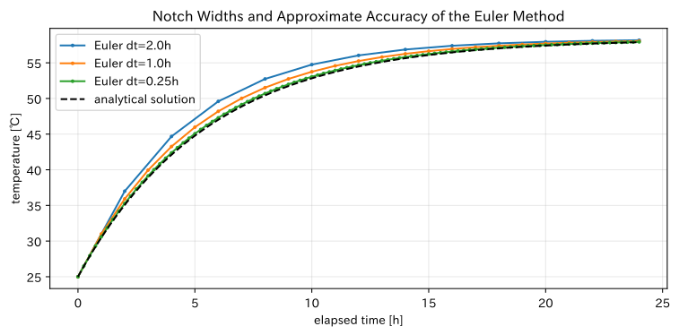
When converting differential equations into spreadsheets or control periods, the most intuitive method is the Euler method. On the other hand, coarse increments carry the risk of overestimating the time to reach the safety limit either too early or too late.

Approach to Analysis and Modeling

Using the tilt of time $t_n$, we predict the next state linearly. The minimum requirement for model verification is “incit width sensitivity analysis,” which halves the indices $\Delta t$ to check if the results remain almost the same.

$T_{n+1}=T_n+\Delta t\,f(t_n,T_n)$

Check with Python

def euler(f, y0, t):
    y = np.empty(len(t), dtype=float)
    y[0] = y0
    for i in range(len(t) - 1):
        dt = t[i + 1] - t[i]
        y[i + 1] = y[i] + dt * f(t[i], y[i])
    return y

f_temp = lambda t, T: heat_input - cooling * (T - T_env)
rows = []
fig, ax = plt.subplots(figsize=(8, 4))
for dt in [2.0, 1.0, 0.25]:
    t = np.arange(0, 24 + dt, dt)
    y = euler(f_temp, 25.0, t)
    exact = T_eq + (25.0 - T_eq) * np.exp(-cooling * t)
    rows.append({"Notch width[h]": dt, "Score Calculation": len(t), "maximum absolute error[℃]": np.max(np.abs(y - exact))})
    ax.plot(t, y, marker="o", markersize=2, label=f"Euler dt={dt}h")
ax.plot(t_eval, T_eq + (25.0 - T_eq) * np.exp(-cooling * t_eval), color="black", linestyle="--", label="analytical solution")
display(pd.DataFrame(rows).round(4))
ax.set_title("Notch Widths and Approximate Accuracy of the Euler Method")
ax.set_xlabel("elapsed time [h]")
ax.set_ylabel("temperature [℃]")
ax.grid(True, alpha=0.3)
ax.legend()
plt.tight_layout()
plt.show()

	Notch width[h]	Score Calculation	maximum absolute error[℃]
0	2.000	13	2.582
1	1.000	25	1.194
2	0.250	97	0.281

Reading the results

The smaller the notch width, the closer it is to the analytical solution. Just because you have hourly data doesn’t mean one hour is enough for calculation intervals. Right after startup or control changes, when temperature changes are rapid, fine-tune the process to balance the computational load.

No.063: Runge-Kutta Method

Meaning in Practice

In long-term forecasting and nonlinear models, errors in the Euler method accumulate. When judging capital investment and safety margins, it is necessary to distinguish between the uncertainties of model structure and numerical errors.

Approach to Analysis and Modeling

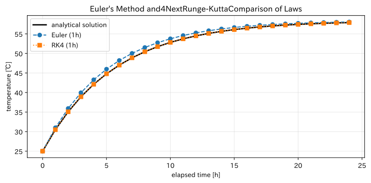
The 4th order Runge-Kutta method (RK4) evaluates slopes at multiple points within a single step and updates them with weighted averages. While the same notch width tends to achieve high precision, four tilt evaluations are required. Methods are chosen not only based on accuracy but also on computation time, explainability, and reproducibility.

$y_{n+1}=y_n+\frac{\Delta t}{6}(k_1+2k_2+2k_3+k_4)$

Check with Python

def rk4(f, y0, t):
    y = np.empty(len(t), dtype=float)
    y[0] = y0
    for i in range(len(t) - 1):
        dt = t[i + 1] - t[i]
        k1 = f(t[i], y[i])
        k2 = f(t[i] + dt/2, y[i] + dt*k1/2)
        k3 = f(t[i] + dt/2, y[i] + dt*k2/2)
        k4 = f(t[i] + dt, y[i] + dt*k3)
        y[i + 1] = y[i] + dt * (k1 + 2*k2 + 2*k3 + k4) / 6
    return y

t_1h = np.arange(0, 25, 1.0)
exact_1h = T_eq + (25.0 - T_eq) * np.exp(-cooling * t_1h)
euler_1h = euler(f_temp, 25.0, t_1h)
rk4_1h = rk4(f_temp, 25.0, t_1h)
comparison_063 = pd.DataFrame({
    "technique": ["Euler", "RK4"],
    "24post-time error[℃]": [abs(euler_1h[-1]-exact_1h[-1]), abs(rk4_1h[-1]-exact_1h[-1])],
    "maximum absolute error[℃]": [np.max(abs(euler_1h-exact_1h)), np.max(abs(rk4_1h-exact_1h))],
})
display(comparison_063.round(6))

fig, ax = plt.subplots(figsize=(8, 4))
ax.plot(t_1h, exact_1h, color="black", linewidth=2, label="analytical solution")
ax.plot(t_1h, euler_1h, "o--", label="Euler (1h)")
ax.plot(t_1h, rk4_1h, "s:", label="RK4 (1h)")
ax.set_title("Euler's Method and4NextRunge-KuttaComparison of Laws")
ax.set_xlabel("elapsed time [h]")
ax.set_ylabel("temperature [℃]")
ax.grid(True, alpha=0.3)
ax.legend()
plt.tight_layout()
plt.show()

	technique	24post-time error[℃]	maximum absolute error[℃]
0	Euler	0.159	1.194
1	RK4	0.000	0.000

Reading the results

Even at hourly increments, RK4’s error is significantly smaller than the Euler method. High-precision methods do not accurately produce coarse input data. If estimation errors in input parameters dominate, the measurement design should be reviewed before improving numerical accuracy.

No.064: Lotka Volterra Model

Meaning in Practice

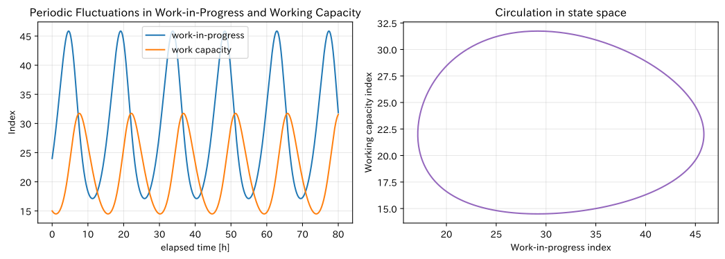
When work-in-progress increases, support personnel are deployed; when work-in-progress decreases, cheering is canceled, creating cyclical fluctuations. Instead of using the classic predator-prey model as a predictor, it is used as teaching material for the structure of ‘circulation.‘

Approach to Analysis and Modeling

Assume that the Work-in-Progress Index $x$ and the Working Capacity Index $y$ influence each other’s rate of change. The coefficient represents the direction of causality and the reaction rate. In practice, non-negative constraints, capability caps, and shift switching are added, and validity is verified using measured data.

$\frac{dx}{dt}=\alpha x-\beta xy,\qquad \frac{dy}{dt}=\delta xy-\gamma y$

Check with Python

# x: Work-in-progress pending processing, y: Supportable work capacity (conceptual model)
alpha, beta, delta, gamma = 0.55, 0.025, 0.012, 0.35
def lv_factory(t, z):
    x, y = z
    return [alpha*x - beta*x*y, delta*x*y - gamma*y]

t_lv = np.linspace(0, 80, 1601)
sol_064 = solve_ivp(lv_factory, [0, 80], [24, 15], t_eval=t_lv, rtol=1e-8, atol=1e-10)
lv_summary = pd.DataFrame({
    "Condition": ["work-in-progress", "work capacity"],
    "smallest": sol_064.y.min(axis=1), "largest": sol_064.y.max(axis=1),
    "average": sol_064.y.mean(axis=1),
})
display(lv_summary.round(2))

fig, axes = plt.subplots(1, 2, figsize=(11, 4))
axes[0].plot(t_lv, sol_064.y[0], label="work-in-progress")
axes[0].plot(t_lv, sol_064.y[1], label="work capacity")
axes[0].set_title("Periodic Fluctuations in Work-in-Progress and Working Capacity")
axes[0].set_xlabel("elapsed time [h]"); axes[0].set_ylabel("Index")
axes[0].grid(True, alpha=0.3); axes[0].legend()
axes[1].plot(sol_064.y[0], sol_064.y[1], color="tab:purple")
axes[1].set_title("Circulation in state space")
axes[1].set_xlabel("Work-in-progress index"); axes[1].set_ylabel("Working capacity index")
axes[1].grid(True, alpha=0.3)
plt.tight_layout()
plt.show()

	Condition	smallest	largest	average
0	work-in-progress	17.120	45.850	29.940
1	work capacity	14.490	31.740	21.860

Reading the results

You can check the cycle in both the time series and state space. The phase difference where work capacity increases after the work-in-progress peak is a typical example of delayed support. Just because the cycle is visible doesn’t mean the model is correct; we verify the structural hypothesis by comparing it with the actual times of support issuance and cancellation.

No.065: SIR Model

Meaning in Practice

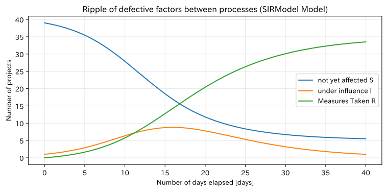
Misalignments in common jigs, incorrect work standards, or abnormalities in material lots can spread across multiple processes. By using the SIR model, the number of processes that are unaffected, currently affected, and countermeasures can be separated, and the required containment speed level can be discussed.

Approach to Analysis and Modeling

All 40 processes are classified as unaffected $S$, affected $I$, or $R$ already addressed. Spread coefficient $\beta$ corresponds to the strength of contact and common factors, while countermeasure coefficient $\gamma$ corresponds to the speed from detection to containment. Also check the parameter save $S+I+R=N$.

$\frac{dS}{dt}=-\beta\frac{SI}{N},\quad \frac{dI}{dt}=\beta\frac{SI}{N}-\gamma I,\quad \frac{dR}{dt}=\gamma I$

Check with Python

# Representing the spread of defective factors in process groups using SIR type
N = 40
beta_sir, gamma_sir = 0.42, 0.18
def sir_quality(t, z):
    S, I, R = z
    new_affected = beta_sir * S * I / N
    contained = gamma_sir * I
    return [-new_affected, new_affected-contained, contained]

t_sir = np.linspace(0, 40, 401)
sol_065 = solve_ivp(sir_quality, [0, 40], [39, 1, 0], t_eval=t_sir)
peak_i = np.argmax(sol_065.y[1])
display(pd.DataFrame({
    "KPI": ["Peak of the Influence Process", "Peak time[days]", "40Unprepared Steps Later"],
    "value": [sol_065.y[1, peak_i], sol_065.t[peak_i], sol_065.y[0, -1]],
}).round(2))

fig, ax = plt.subplots(figsize=(8, 4))
ax.plot(t_sir, sol_065.y[0], label="not yet affected S")
ax.plot(t_sir, sol_065.y[1], label="under influence I")
ax.plot(t_sir, sol_065.y[2], label="Measures Taken R")
ax.set_title("Ripple of defective factors between processes (SIRModel Model)")
ax.set_xlabel("Number of days elapsed [days]")
ax.set_ylabel("Number of projects")
ax.grid(True, alpha=0.3)
ax.legend()
plt.tight_layout()
plt.show()

	KPI	value
0	Peak of the Influence Process	8.800
1	Peak time[days]	16.000
2	40Unprepared Steps Later	5.500

Reading the results

There is a peak in the affected process, and it is necessary to secure inspection capacity and alternative processes by that point. Measures to enhance $\gamma$ include initial contact, traceability, and immediate updates of standard work. Because there is a simplification to uniformly handle non-independent processes, in practice it extends to the spillover rate by process network.

No.066: System Dynamics

Meaning in Practice

System dynamics clearly represent stocks like work-in-progress and inventory, as well as flows like input and completion. Rather than tracking KPIs individually, it is effective for capturing the overall picture, including causality and time lag.

Approach to Analysis and Modeling

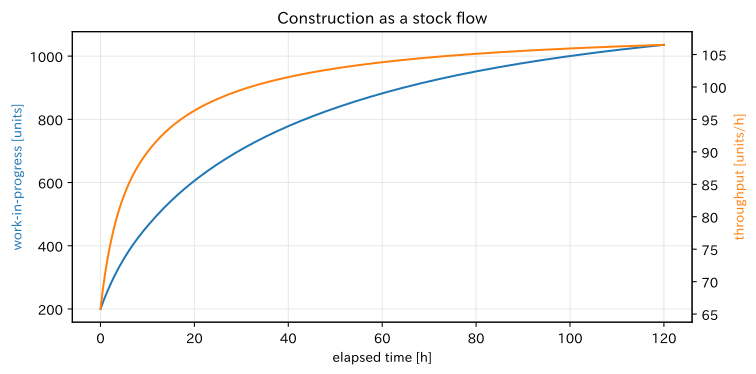
Work-in-progress $W$ varies depending on the feed rate and throughput. Here, if there are few work-in-progress, the capacity cannot be fully utilized due to waiting for parts; the more work-in-progress, the closer the capacity is reached, using a saturation function. Parameters can be estimated from input records, completion records, and work-in-progress inventory.

$\frac{dW}{dt}=r_{\mathrm{in}}-r_{\mathrm{out}},\qquad r_{\mathrm{out}}=C_{\max}\frac{W}{K+W}$

Check with Python

# On the work-in-progress stock, both the input inflow and the finished outflow act
arrival_rate, max_capacity, half_saturation = 108.0, 125.0, 180.0
def wip_ode(t, z):
    wip = z[0]
    throughput = max_capacity * wip / (half_saturation + wip)
    return [arrival_rate - throughput]

t_sd = np.linspace(0, 120, 481)
sol_066 = solve_ivp(wip_ode, [0, 120], [200], t_eval=t_sd)
throughput_066 = max_capacity * sol_066.y[0] / (half_saturation + sol_066.y[0])
display(pd.DataFrame({
    "KPI": ["Initial work-in-progress", "120work-in-progress after time", "120After-hours throughput"],
    "value": [sol_066.y[0,0], sol_066.y[0,-1], throughput_066[-1]],
    "Unit": ["units", "units", "units/h"],
}).round(2))

fig, ax1 = plt.subplots(figsize=(8, 4))
ax1.plot(t_sd, sol_066.y[0], color="tab:blue", label="work-in-progress")
ax1.set_xlabel("elapsed time [h]"); ax1.set_ylabel("work-in-progress [units]", color="tab:blue")
ax2 = ax1.twinx()
ax2.plot(t_sd, throughput_066, color="tab:orange", label="throughput")
ax2.set_ylabel("throughput [units/h]", color="tab:orange")
ax1.set_title("Construction as a stock flow")
ax1.grid(True, alpha=0.3)
fig.tight_layout()
plt.show()

	KPI	value	Unit
0	Initial work-in-progress	200.000	units
1	120work-in-progress after time	1035.760	units
2	120After-hours throughput	106.490	units/h

Reading the results

As the feed rate exceeds the initial throughput, work-in-progress increases, but as the workload grows, the completion rate also rises, eventually reaching equilibrium. Increasing work-in-progress is not always better; near maximum capacity, the effect of additional work-in-progress is small, resulting in burdens of stagnation, quality, and operating costs.

No.067: Inventory Dynamics

Meaning in Practice

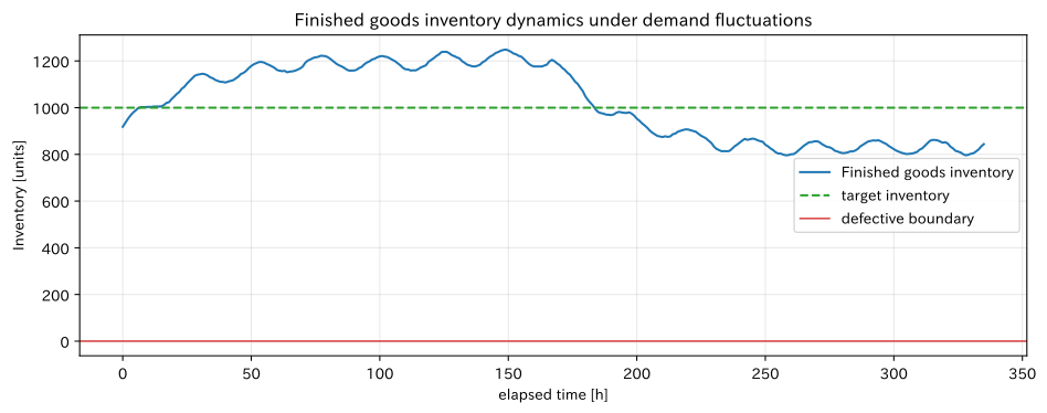
Finished goods inventory absorbs fluctuations in demand, but there is an upper limit to increased production. By looking at not only inventory standards but also minimum inventory, out-of-stock duration, and production leveling simultaneously, you can determine the trade-off between service levels and operational load.

Approach to Analysis and Modeling

Inventory $I$ is updated by the difference between production $P$ and demand $D$. Production is adjusted for inventory deviations on top of the standard quantity, and the upper and lower limits of equipment capacity are cut. If demand cannot be met, negative inventory is interpreted as backlog.

$\frac{dI}{dt}=P(t)-D(t),\qquad P(t)=\mathrm{clip}\{P_0+g(I^*-I),P_{\min},P_{\max}\}$

Check with Python

def simulate_inventory(gain, initial_inventory=900.0):
    inv = np.empty(len(hours) + 1)
    prod = np.empty(len(hours))
    inv[0] = initial_inventory
    target = 1000.0
    for i, d in enumerate(demand):
        prod[i] = np.clip(108 + gain * (target - inv[i]), 85, 130)
        inv[i+1] = inv[i] + prod[i] - d
    return inv, prod

inv_067, prod_067 = simulate_inventory(gain=0.04)
shortage_hours = int(np.sum(inv_067[1:] < 0))
display(pd.DataFrame({
    "KPI": ["ending inventory", "Minimum stock", "Shortage time", "Average production volume"],
    "value": [inv_067[-1], inv_067.min(), shortage_hours, prod_067.mean()],
    "Unit": ["units", "units", "h", "units/h"],
}).round(2))

fig, ax = plt.subplots(figsize=(10, 4))
ax.plot(hours, inv_067[1:], label="Finished goods inventory")
ax.axhline(1000, color="tab:green", linestyle="--", label="target inventory")
ax.axhline(0, color="tab:red", linewidth=1, label="defective boundary")
ax.set_title("Finished goods inventory dynamics under demand fluctuations")
ax.set_xlabel("elapsed time [h]")
ax.set_ylabel("Inventory [units]")
ax.grid(True, alpha=0.3)
ax.legend()
plt.tight_layout()
plt.show()

	KPI	value	Unit
0	ending inventory	843.920	units
1	Minimum stock	796.080	units
2	Shortage time	0.000	h
3	Average production volume	107.200	units/h

Reading the results

After promotions, demand rises and inventory decreases, and control rules encourage increased production. Even if there is zero out-of-stock time, if the minimum inventory is small, there is little margin for forecast error. It should be evaluated under multiple scenarios varying safety stock, cap capacity, and overtime costs.

No.068: Demand Dynamics

Meaning in Practice

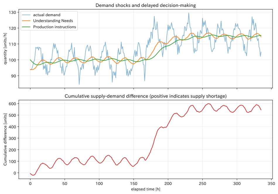
Changes in demand do not immediately transmit to production. When aggregation, approvals, planning freezes, and procurement lead delays accumulate, production remains at old levels for some time even after demand increases, leading to a widening cumulative shortfall.

Approach to Analysis and Modeling

From actual demand $D$ to recognized demand $\hat D$, and further to production order $O$, the primary delay is connected in two stages. The time constant $\tau$ represents the speed of the reaction; the smaller the case, the faster the follow-up. The cumulative supply-demand gap corresponds to the required inventory buffer and the size of the backlog of orders.

$\frac{d\hat D}{dt}=\frac{D-\hat D}{\tau_D},\qquad \frac{dO}{dt}=\frac{\hat D-O}{\tau_O}$

Check with Python

# Exponentially smoothed perceived demand and production instructions follow behind actual demand.
perceived = np.empty(len(hours))
order = np.empty(len(hours))
perceived[0], order[0] = demand[0], 100.0
tau_perception, tau_order = 18.0, 12.0
for i in range(1, len(hours)):
    perceived[i] = perceived[i-1] + (demand[i-1] - perceived[i-1]) / tau_perception
    order[i] = order[i-1] + (perceived[i-1] - order[i-1]) / tau_order

cumulative_gap = np.cumsum(demand - order)
display(pd.DataFrame({
    "KPI": ["Average post-promotion demand", "Post-promotion Average Production Instructions", "Maximum cumulative supply-demand difference"],
    "value": [demand[168:].mean(), order[168:].mean(), cumulative_gap.max()],
    "Unit": ["units/h", "units/h", "units"],
}).round(2))

fig, axes = plt.subplots(2, 1, figsize=(10, 7), sharex=True)
axes[0].plot(hours, demand, alpha=0.55, label="actual demand")
axes[0].plot(hours, perceived, label="Understanding Needs")
axes[0].plot(hours, order, label="Production instructions")
axes[0].set_title("Demand shocks and delayed decision-making")
axes[0].set_ylabel("quantity [units/h]"); axes[0].grid(True, alpha=0.3); axes[0].legend()
axes[1].plot(hours, cumulative_gap, color="tab:red")
axes[1].set_title("Cumulative supply-demand difference (positive indicates supply shortage)")
axes[1].set_xlabel("elapsed time [h]"); axes[1].set_ylabel("Cumulative difference [units]"); axes[1].grid(True, alpha=0.3)
plt.tight_layout()
plt.show()

	KPI	value	Unit
0	Average post-promotion demand	114.780	units/h
1	Post-promotion Average Production Instructions	112.180	units/h
2	Maximum cumulative supply-demand difference	598.950	units

Reading the results

After the promotion begins, awareness demand and production instructions gradually lag behind, leading to an increase in cumulative shortages. Countermeasures include not only simple production increases, but also early sharing of promotional information, shortening freeze periods, and advancing material procurement. Time constants are set not by meeting frequency, but by the actual lead time from information generation to execution.

No.069: Feedback Loop

Meaning in Practice

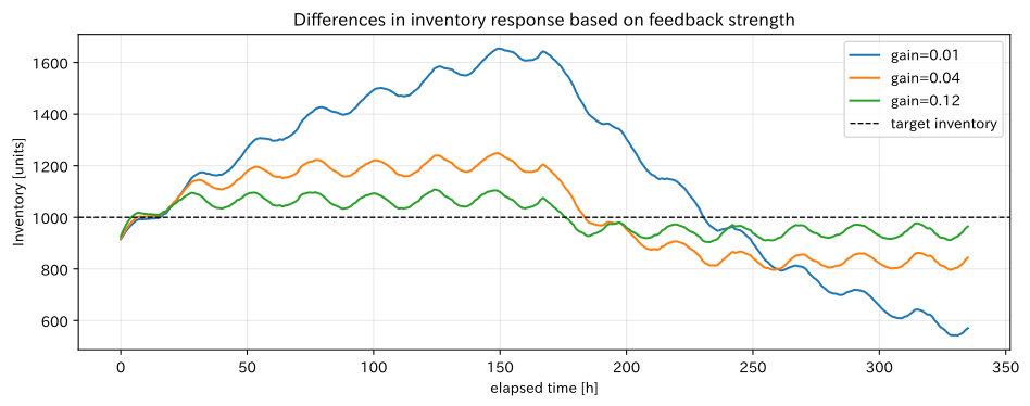
Negative feedback to adjust production based on inventory deviations is fundamental to reducing stockouts. However, if the response is too strong, fluctuations in production volume, overtime, and setup changes increase, and delays can amplify inventory fluctuations.

Approach to Analysis and Modeling

Using the inventory adjustment factor $g$ as a policy variable, we compare three cases: weak, medium, and strong. The evaluation includes not only upper and lower limits of inventory but also the standard deviation of production volume. In practice, we select robust coefficient ranges after accounting for capability constraints and delayed decision-making.

$P=P_0+g(I^*-I)\quad (g>0)$

Check with Python

feedback_rows = []
fig, ax = plt.subplots(figsize=(10, 4))
for gain in [0.01, 0.04, 0.12]:
    inv, prod = simulate_inventory(gain=gain)
    feedback_rows.append({
        "feedback coefficient": gain,
        "Minimum stock[units]": inv.min(),
        "Maximum inventory[units]": inv.max(),
        "Production volume standard deviation[units/h]": prod.std(),
        "Shortage time[h]": np.sum(inv[1:] < 0),
    })
    ax.plot(hours, inv[1:], label=f"gain={gain}")
display(pd.DataFrame(feedback_rows).round(2))
ax.axhline(1000, color="black", linestyle="--", linewidth=1, label="target inventory")
ax.set_title("Differences in inventory response based on feedback strength")
ax.set_xlabel("elapsed time [h]")
ax.set_ylabel("Inventory [units]")
ax.grid(True, alpha=0.3)
ax.legend()
plt.tight_layout()
plt.show()

	feedback coefficient	Minimum stock[units]	Maximum inventory[units]	Production volume standard deviation[units/h]	Shortage time[h]
0	0.010	542.260	1653.650	3.360	0
1	0.040	796.080	1248.940	6.410	0
2	0.120	900.000	1108.140	7.590	0

Reading the results

Increasing the coefficient tends to speed up return to target inventory, while increasing fluctuations in production volume. The optimal coefficient cannot be determined by a single KPI. It is necessary to compare shortage losses, overtime costs, setup losses, and inventory interest by converting them into common cost units.

No.070: Stability of Simulation

Meaning in Practice

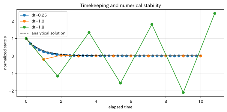
Graph vibrations and divergence can occur not due to instability on site, but due to calculation methods. To avoid incorrect capital investments and control changes, numerical stability is verified separately from model validity.

Approach to Analysis and Modeling

If you solve the damping system $dy/dt=-\lambda y$ using the positive Euler method, the amplification rate per update is $1-\lambda\Delta t$. If the absolute value is less than 1, the error will be attenuated. We also check that KPIs converge by adjusting the increment width.

$y_{n+1}=(1-\lambda\Delta t)y_n,\qquad |1-\lambda\Delta t|<1$

Check with Python

# Calculate dy/dt = -lambda*y using the positive Euler method. The stability condition is |1-lambda*dt| < 1
lam, y0, horizon = 1.2, 1.0, 10.0
stability_rows = []
fig, ax = plt.subplots(figsize=(8, 4))
for dt in [0.25, 1.0, 1.8]:
    t = np.arange(0, horizon + dt, dt)
    y = euler(lambda t, y: -lam*y, y0, t)
    factor = 1 - lam*dt
    stability_rows.append({
        "Notch widthdt": dt, "amplification rate(1-λdt)": factor,
        "Theoretically stable": abs(factor) < 1, "maximum absolute value": np.max(np.abs(y)),
    })
    ax.plot(t, y, marker="o", label=f"dt={dt}")
t_exact = np.linspace(0, horizon, 301)
ax.plot(t_exact, np.exp(-lam*t_exact), color="black", linestyle="--", label="analytical solution")
display(pd.DataFrame(stability_rows).round(3))
ax.set_title("Timekeeping and numerical stability")
ax.set_xlabel("elapsed time")
ax.set_ylabel("normalized state y")
ax.grid(True, alpha=0.3)
ax.legend()
plt.tight_layout()
plt.show()

	Notch widthdt	amplification rate(1-λdt)	Theoretically stable	maximum absolute value
0	0.250	0.700	True	1.000
1	1.000	-0.200	True	1.000
2	1.800	-1.160	False	2.436

Reading the results

At fine increments, it attenuates smoothly, while in moderate increments, it changes the code while attenuating. In coarse cuts that do not meet stable conditions, the attenuation system appears to be diverging. For public and approval models, we record the adopted solver, tolerance of error, increment width sensitivity, and reproduction environment.

Practical Implications Seen Through Target Exercise

1. Separate state and flow rate: Inventory, work-in-progress, and equipment condition are stock, while ordering, production, deterioration, and recovery are part of the flow. It is important not to confuse the two even in meeting materials.
2. DelayKPIto become: By measuring delays in demand recognition, approval, procurement, and ramp-up in time, you can improve out-of-stock issues rather than just “predicting accuracy.”
3. Look at the trajectory, not the average: Even if the average inventory is appropriate, temporary stockouts or sticking to the cap limit can still carry operational risk.
4. The strength of control has side effects.: Measures to accelerate inventory recovery may increase production fluctuations and on-site workload. Evaluation is conducted using multiple KPIs.
5. Separating numerical errors: Change the notch width and solution method to check if the results converge, distinguishing between phenomena and computational instability.

What is necessary for practical implementation

item	Minimum Essentials	Practical Considerations
Purpose	Target decision-making, KPIs, and comparative scenarios	Don’t just “recreate the current situation”
Data	Time, inventory, input, completion, demand, stop	Unify timestamps and units
Model	Boundaries, states, flows, constraints, delays	Confirm the direction of cause and effect through on-site reviews
presumption	Parameter basis, duration, error	Distinguishing between normal and abnormal states
verification	Holdout period, sensitivity analysis, extreme conditions	Check numerical stability separately
Utilization	Update frequency, responsible persons, criteria for decision-making, version management	Determining the path from result to execution

In PoCs, narrowing the scope to a single product group and one decision, and running short cycles of past repetitions, counter-realistic virtual scenarios, and on-site reviews, makes progress easier.

Conclusion

From No.061 to No.070, we covered everything from formulating differential equations to the Euler method and RK4, interactions, ripples, stock-flow, inventory and demand dynamics, feedback, and numerical stability. The value of continuous simulation lies not in predicting the future in a single point, but in sharing assumptions and causality, allowing you to compare the results and risks of proposed changes before the actual machine is deployed.

To translate analysis results into decision-making, it is essential not only to design model accuracy but also to address on-site constraints, trade-offs between KPIs, and the update and approval processes.

Consultations for Corporations

At Suri Kobo, we support simulation design for manufacturing, inventory and production planning, what-if analysis of capital investment, digital twin construction, and in-house training. You can proceed step by step, from organizing issues and reviewing data, to PoCs of models usable for decision-making and operational implementation.

📩 Contact Us: surikobo.co.jp/contact
Please feel free to consult us first.