Grasping the “Next” of Equipment Through Probability: 10 Exercise-Off Probabilistic Process Simulations in Manufacturing (No.071–No.080)

Title & Overview

Equipment fluctuates between normal, deteriorate, and malfunctioning, with breakdowns and orders occurring irregularly, and sensor readings often contain noise. In this article, we implement probabilistic processes that handle such Uncertainty that changes over time using a fictional precision parts factory as the subject.

Through No.071 to No.080, we connect condition transitions, long-term operating rates, abnormal signs, number of failures, parts replacement, external pricing, equipment deterioration, and sequential condition estimation to support maintenance, inventory, and investment decisions.

[!NOTE] This material is a notebook previously used by Surikoubo (or personally by the representative, Kazuyama), and has been reconstructed, edited, and published with the company’s permission.
All data listed is fictional and has no relation whatsoever to real companies, factories, or figures.

Introduction: Practical Challenges in Manufacturing Covered in This Article

The target is decision-making that reduces sudden stoppages of major processing equipment while avoiding excessive maintenance and inspection man-hours. Mean failure intervals alone cannot answer questions such as “What will happen next to equipment currently in a deteriorating state?”, “What is the probability that the number of failures will increase next month?”, or “How can the true state be estimated from sensors containing noise?”

In this article, we will treat stochastic processes not as a technique for guessing a single prediction value, but as a A decision-making platform for comparing multiple future scenarios and their probabilities.

Common situations on site

• Although the equipment ledger contains a history of failures, the transition structure between normal, deteriorate, and fault is not organized
• You can know the average number of breakdowns per month, but you can’t know the probability of missing maintenance items.
• Vibration and temperature threshold monitoring often results in false alarms and missed spots
• Fluctuations in market prices and demand are not included in sensitivity analysis for capital investment evaluation.
• Even with advanced models, the rationale for parameters and update procedures remain in operation

Why is this issue so difficult to judge?

Even if the average value is the same, differences in occurrence variability, dependence on state status, and observed noise will affect the required countermeasures. In stochastic processes, the state at point $t$ is set as the random variable $X_t$, and the entire sequence $(X_t)_{t\geq0}$ is handled.

In practice, it is important to design (1) what defines a state, (2) whether time is handled discrete or continuous, (3) how to estimate unobservable states, and (4) how to incorporate estimation error into decision-making. It is necessary to evaluate not only model accuracy but also asymmetric losses such as downtime, inspection costs, and out-of-stock costs.

Overview of Exercise covered this time

No.	Theme	Questions in the Manufacturing Industry	Main Outputs
071	Markov chain	How will the equipment status transition into the next term?	Transition of State Probability
072	steady distribution	What is the long-term failure and deterioration ratio?	Long-term state ratio
073	Hidden Markov Model	Can we estimate deterioration that is invisible from the sensor?	Filter probability
074	Poisson process	How many malfunctions and calls will there be?	Number of cases distribution
075	Update Process	How many parts are replaced and replaced?	Number of updates and intervals
076	Brownian motion	How to represent the fluctuation of cumulative error?	Route distribution
077	Geometric Brownian motion	How to evaluate the ratio fluctuations of external prices	Price Scenario
078	Probability differential equation	How to represent the mean regression facility indicator?	Degradation Indicator Pathway
079	Kalman filter	Can continuous states be estimated excluding noise?	Estimated Values and Sections
080	particle filter	Can state estimates be made even with nonlinear observations?	Particle Distribution and Estimated Values

Preparing the Python environment

It does not depend on external data and uses only NumPy, pandas, and matplotlib. The random number generator is initialized with a fixed seed, and rerunning it ensures the same result. Labels in the graph are displayed in English to avoid environmental differences during Markdown conversion.

%matplotlib inline
import sys
import numpy as np
import pandas as pd
import matplotlib
import matplotlib.pyplot as plt
from IPython.display import display

SEED = 20260712
rng = np.random.default_rng(SEED)
plt.rcParams.update({"figure.figsize": (8, 4), "axes.grid": True})
print(f"Python     : {sys.version.split()[0]}")
print(f"NumPy      : {np.__version__}")
print(f"pandas     : {pd.__version__}")
print(f"matplotlib : {matplotlib.__version__}")
print(f"random seed: {SEED}")

Python     : 3.13.1
NumPy      : 2.5.1
pandas     : 3.0.3
matplotlib : 3.11.0
random seed: 20260712

Creation of Fictional Data

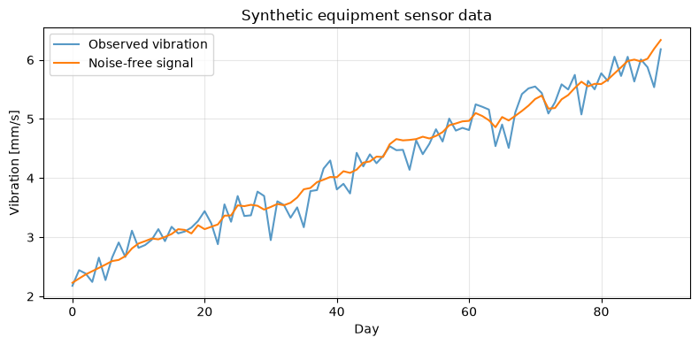
Assuming the main processing equipment of a precision parts factory, it generates 90 days’ worth of “true deterioration” and vibration sensor values. The true degree of degradation is kept only for verification and is a latent state that cannot be observed in actual operation. In the latter part of the filter, this state is estimated based solely on observations.

days = 90
t = np.arange(days)
true_health = np.zeros(days)
true_health[0] = 1.0
for i in range(1, days):
    true_health[i] = max(0, true_health[i-1] + 0.025 + rng.normal(0, 0.045))
vibration = 1.2 + 0.85 * true_health + 0.18 * true_health**2 + rng.normal(0, 0.22, days)
temperature = 42 + 3.2 * true_health + rng.normal(0, 0.8, days)
sensor_df = pd.DataFrame({"day": t, "true_degradation": true_health,
                          "vibration_mm_s": vibration, "temperature_C": temperature})
display(sensor_df.head().round(3))
print(f"rows={len(sensor_df)}, missing={sensor_df.isna().sum().sum()}")

fig, ax = plt.subplots()
ax.plot(t, vibration, label="Observed vibration", alpha=0.75)
ax.plot(t, 1.2 + 0.85*true_health + 0.18*true_health**2, label="Noise-free signal")
ax.set_title("Synthetic equipment sensor data")
ax.set_xlabel("Day"); ax.set_ylabel("Vibration [mm/s]")
ax.grid(True, alpha=.3); ax.legend(); plt.tight_layout(); plt.show()

	day	true_degradation	vibration_mm_s	temperature_C
0	0	1.000	2.179	44.119
1	1	1.058	2.443	46.809
2	2	1.114	2.385	45.303
3	3	1.158	2.244	44.773
4	4	1.201	2.654	45.412

rows=90, missing=0

No.071: Predicting Equipment Condition Changes Using Markov Chains

Meaning in Practice

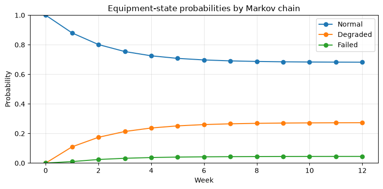
The equipment condition during inspection is divided into three levels: Normal, Degraded, and Failed, and the probability of the next week’s condition is predicted. Instead of a single prediction of “failure/non-failure,” the conservation plan can be shared as the probability of downtime risk.

Approach to Analysis and Modeling

The Markov chain is an approximation that “the next state depends only on the current state.” When you define element $p_{ij}=P(X_{t+1}=j\mid X_t=i)$ of the transition matrix $P$, the state probability vector is updated at $\boldsymbol{\pi}_{t+1}=\boldsymbol{\pi}_tP$. After a malfunction, repairs will restore it to normal or deteriorate settings.

Check with Python

states = ["Normal", "Degraded", "Failed"]
P = np.array([[0.88, 0.11, 0.01], [0.18, 0.68, 0.14], [0.72, 0.28, 0.00]])
display(pd.DataFrame(P, index=states, columns=states).style.format("{:.0%}"))
pi = np.array([1.0, 0.0, 0.0])
history = [pi.copy()]
for _ in range(12):
    pi = pi @ P
    history.append(pi.copy())
markov_df = pd.DataFrame(history, columns=states).assign(week=np.arange(13))
display(markov_df.iloc[[0, 1, 4, 8, 12]].set_index("week").round(4))
fig, ax = plt.subplots()
for s in states: ax.plot(markov_df.week, markov_df[s], marker="o", label=s)
ax.set_title("Equipment-state probabilities by Markov chain")
ax.set_xlabel("Week"); ax.set_ylabel("Probability")
ax.set_ylim(0, 1); ax.grid(True, alpha=.3); ax.legend(); plt.tight_layout(); plt.show()

	Normal	Degraded	Failed
Normal	88%	11%	1%
Degraded	18%	68%	14%
Failed	72%	28%	0%

	Normal	Degraded	Failed
week
0	1.0000	0.0000	0.0000
1	0.8800	0.1100	0.0100
4	0.7253	0.2372	0.0374
8	0.6872	0.2687	0.0441
12	0.6820	0.2730	0.0450

Reading the results

Even if it starts normally, as time progresses, the probability of deterioration and failure accumulates, eventually approaching a certain configuration ratio. By showing the probability of failure not only the following week but also 4 to 12 weeks ahead, you can advance spare parts and secure planned downtime slots. However, if equipment age or load are strongly affected, it is necessary to subdivide the condition or apply time-dependent transition probabilities.

No.072: Estimating Long-Term Facility State Ratios Using Steady-State Distribution

Meaning in Practice

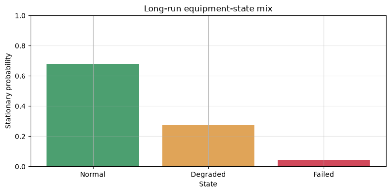
Estimate what percentage of equipment will be normal, deteriorated, or fail if the same operation continues for a long time. It serves as a baseline for long-term maintenance personnel, replacement capacity, and downtime losses.

Approach to Analysis and Modeling

The stationary distribution $\boldsymbol{\pi}^*$ satisfies $\boldsymbol{\pi}^*=\boldsymbol{\pi}^*P$ and $\sum_i\pi_i^*=1$. Under conditions where the initial state converges to the same distribution, long-term KPIs unaffected by fluctuations in short-term simulations can be obtained.

Check with Python

A = np.vstack([P.T - np.eye(len(states)), np.ones(len(states))])
b = np.r_[np.zeros(len(states)), 1.0]
stationary, *_ = np.linalg.lstsq(A, b, rcond=None)
stationary_df = pd.DataFrame({"state": states, "stationary_probability": stationary})
display(stationary_df.style.format({"stationary_probability": "{:.2%}"}))
weekly_loss = np.array([0, 350_000, 2_400_000])
expected_loss = stationary @ weekly_loss
print(f"Long-run expected weekly loss: JPY {expected_loss:,.0f}")
fig, ax = plt.subplots()
ax.bar(states, stationary, color=["#4c9f70", "#e0a458", "#d1495b"])
ax.set_title("Long-run equipment-state mix")
ax.set_xlabel("State"); ax.set_ylabel("Stationary probability")
ax.set_ylim(0, 1); ax.grid(True, axis="y", alpha=.3); plt.tight_layout(); plt.show()

	state	stationary_probability
0	Normal	68.12%
1	Degraded	27.37%
2	Failed	4.51%

Long-run expected weekly loss: JPY 204,076

Reading the results

By multiplying the steady-state deterioration and failure ratio by the weekly loss by the state-specific loss, you can calculate the long-term expected loss. The same calculation is performed for the transition matrix after the conservation policy change, and by comparing the expected loss reduction amount with the cost of the policy, investment decisions are made. The steady distribution is not a “forecast of the week,” but a long-term standard without changing operational rules.

No.073: Estimating Potential Degradation with the Hidden Markov Model

Meaning in Practice

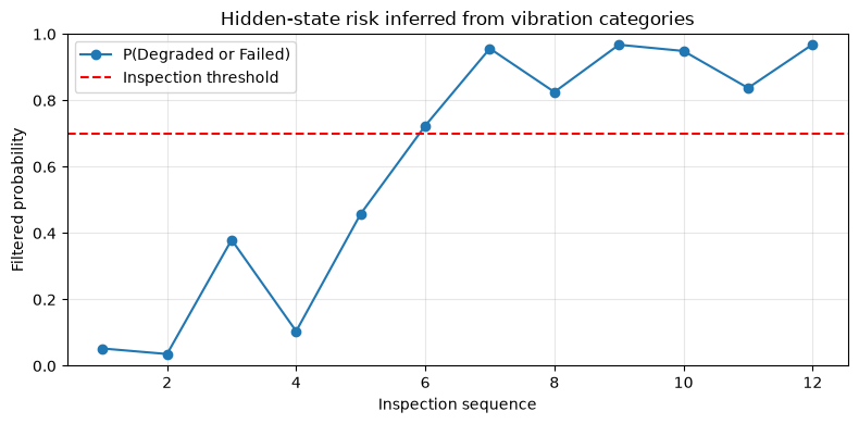
This is a situation where the true condition of the equipment is not directly visible, and only vibration judgments (Low / Medium / High) are observed. It does not respond to single anomalies, and can update the degradation probability including past observation series.

Approach to Analysis and Modeling

The Hidden Markov Model (HMM) combines the transition probabilities of latent states with the observational probabilities for each state. The forward filter iterates between forecast $\hat{\alpha}_t=\alpha_{t-1}P$ and observational correction $\alpha_t\propto\hat{\alpha}_t\odot b(y_t)$.

Check with Python

emissions = np.array([[0.82, 0.16, 0.02], [0.18, 0.62, 0.20], [0.03, 0.22, 0.75]])
obs_names = ["Low", "Medium", "High"]
observations = np.array([0,0,1,0,1,1,2,1,2,2,1,2])
alpha = np.array([0.85, 0.14, 0.01])
filtered = []
for y in observations:
    pred = alpha @ P
    alpha = pred * emissions[:, y]
    alpha /= alpha.sum()
    filtered.append(alpha.copy())
hmm_df = pd.DataFrame(filtered, columns=states)
hmm_df["observation"] = [obs_names[i] for i in observations]
hmm_df.index = np.arange(1, len(hmm_df)+1)
display(hmm_df.tail().round(3))
fig, ax = plt.subplots()
ax.plot(hmm_df.index, hmm_df.Degraded + hmm_df.Failed, marker="o", label="P(Degraded or Failed)")
ax.axhline(.7, color="red", linestyle="--", label="Inspection threshold")
ax.set_title("Hidden-state risk inferred from vibration categories")
ax.set_xlabel("Inspection sequence"); ax.set_ylabel("Filtered probability")
ax.set_ylim(0,1); ax.grid(True, alpha=.3); ax.legend(); plt.tight_layout(); plt.show()

	Normal	Degraded	Failed	observation
8	0.175	0.782	0.044	Medium
9	0.032	0.556	0.412	High
10	0.051	0.597	0.352	High
11	0.162	0.791	0.046	Medium
12	0.031	0.556	0.412	High

Reading the results

If high observations continue, the probability of degradation or malfunction after the event increases, and relying only on the intermediate medium will not suddenly return to normal. For example, a 70% risk probability can be used as the standard for precision inspections. The threshold should be set not by false alarm rate, but by comparing the downtime loss at missed moments with inspection costs.

No.074: Estimating the Number of Fault Calls During the Poisson Process

Meaning in Practice

We model the number of fault calls occurring at a constant rate from independent equipment groups to calculate the probability of shortages in maintenance personnel and spare parts.

Approach to Analysis and Modeling

In a Poisson process with an incidence rate of $\lambda$ per unit time, the number of events $N(t)$ for period $t$ follows $P(N(t)=k)=e^{-\lambda t}(\lambda t)^k/k!$, and the interval between arrivals follows an exponential distribution of average $1/\lambda$. If the incidence rate changes with season or shift, extend to non-uniform Poisson processes and similar processes.

Check with Python

lambda_day = 0.42
sim_counts = rng.poisson(lambda_day * 30, size=20_000)
spares = 17
summary = pd.Series(sim_counts).describe(percentiles=[.5,.8,.9,.95,.99]).to_frame("30-day failures")
display(summary.round(2))
print(f"P(failures > {spares} spares) = {(sim_counts > spares).mean():.2%}")
fig, ax = plt.subplots()
bins = np.arange(sim_counts.min(), sim_counts.max()+2)-.5
ax.hist(sim_counts, bins=bins, density=True, color="#4c78a8", alpha=.8)
ax.axvline(spares, color="red", linestyle="--", label=f"Spare stock={spares}")
ax.set_title("Simulated monthly failure-call count")
ax.set_xlabel("Failures in 30 days"); ax.set_ylabel("Probability density")
ax.grid(True, axis="y", alpha=.3); ax.legend(); plt.tight_layout(); plt.show()

	30-day failures
count	20000.00
mean	12.60
std	3.55
min	1.00
50%	12.00
80%	16.00
90%	17.00
95%	19.00
99%	21.00
max	28.00

P(failures > 17 spares) = 8.95%

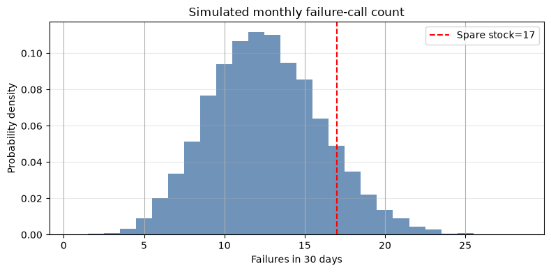
Reading the results

If you only use the average number of cases as inventory numbers, you may run short in about half the months. By listing both quantile and out-of-stock probabilities, you can discuss service levels by service level, such as “inventory covering 95% of the month.” If failures are casual, there are common causes across equipment, or the incidence rate is rising, caution is needed as the Poisson Assumption is underestimated.

No.075: Reproducing the Lifecycle of Replacement Parts During Renewal

Meaning in Practice

After a failure or replacement, the lifespan of the part is reset and it is used again. Model this repetition and estimate the number of annual replacements and budget.

Approach to Analysis and Modeling

For an independent and identically distributed lifetime of $T_1,T_2,\ldots$, the update point is $S_n=\sum_{i=1}^nT_i$, and the number of updates up to time $t$ is $N(t)=\max\{n:S_n\le t\}$. Here, we use the Weibull distribution, which is easier to represent variations in lifespan.

Check with Python

shape, scale = 2.3, 95.0
def renewal_count(horizon, generator):
    elapsed = 0.0; count = 0; times = []
    while True:
        elapsed += scale * generator.weibull(shape)
        if elapsed > horizon: break
        count += 1; times.append(elapsed)
    return count, times
renewals = np.array([renewal_count(365, rng)[0] for _ in range(10_000)])
one_count, one_times = renewal_count(365, np.random.default_rng(SEED+1))
display(pd.Series(renewals).value_counts(normalize=True).sort_index().rename("probability").to_frame().style.format("{:.2%}"))
print(f"Expected annual replacements: {renewals.mean():.2f}")
fig, ax = plt.subplots()
ax.step([0]+one_times+[365], np.arange(one_count+2), where="post")
ax.scatter(one_times, np.arange(1, one_count+1), color="red", zorder=3)
ax.set_title("One sample path of component renewals")
ax.set_xlabel("Day"); ax.set_ylabel("Cumulative replacements")
ax.grid(True, alpha=.3); plt.tight_layout(); plt.show()

	probability
1	0.07%
2	5.21%
3	28.66%
4	38.92%
5	19.98%
6	6.07%
7	0.98%
8	0.11%

Expected annual replacements: 3.96

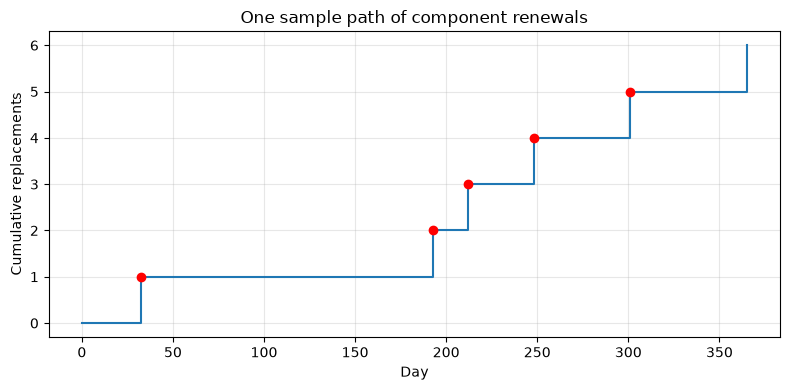
Reading the results

The number of replacements can be tracked not only by average but also by distribution, allowing you to assess the annual budget upward and the required quantity of maintenance items. If there are repairs that do not return to the same condition as new, preventive replacements, or dependent failures of multiple parts, the process is extended from simple updates to virtual age models and competitive risks.

No.076: Represents the Minute Fluctuations Accumulated in Brownian Motion

Meaning in Practice

The uncertainty of quantity caused by many small influences, such as dimensional correction errors and thermal displacement, is evaluated as a pathway.

Approach to Analysis and Modeling

The standard Brownian motion $W_t$ is $W_0=0$, has independent increments, and is $W_{t+\Delta t}-W_t\sim N(0,\Delta t)$. If you consider the drifted process $X_t=\mu t+\sigma W_t$, systematic deviations and random fluctuations can be separated. However, physical boundaries and mean regression are not included.

Check with Python

n_paths, n_steps, horizon = 5000, 120, 8.0
dt = horizon / n_steps
mu, sigma = 0.018, 0.085
increments = mu*dt + sigma*np.sqrt(dt)*rng.normal(size=(n_paths, n_steps))
paths = np.c_[np.zeros(n_paths), np.cumsum(increments, axis=1)]
time = np.linspace(0, horizon, n_steps+1)
limit = 0.30
print(f"P(|error at horizon| > {limit:.2f}) = {(np.abs(paths[:,-1]) > limit).mean():.2%}")
fig, ax = plt.subplots()
for p in paths[:30]: ax.plot(time, p, color="#4c78a8", alpha=.18)
q05, q50, q95 = np.quantile(paths, [.05,.5,.95], axis=0)
ax.plot(time, q50, color="black", label="Median")
ax.fill_between(time, q05, q95, alpha=.25, label="90% range")
ax.axhline(limit, color="red", linestyle="--"); ax.axhline(-limit, color="red", linestyle="--")
ax.set_title("Accumulated process error under Brownian motion")
ax.set_xlabel("Operating time [h]"); ax.set_ylabel("Accumulated error [mm]")
ax.grid(True, alpha=.3); ax.legend(); plt.tight_layout(); plt.show()

P(|error at horizon| > 0.30) = 29.82%

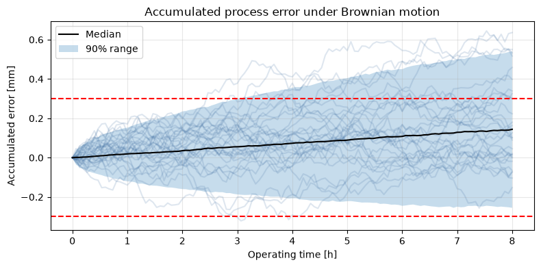
Reading the results

You can check not only the probability of non-standard at the end of the workday but also the route along the way and within the 90% range. The calibration interval can be designed based on times exceeding the allowable risk. On the other hand, in control systems where errors return to the center, Brownian motion overestimates long-term variance, so the mean regression model No.078 is more suitable.

No.077: Creating External Price Scenarios with Geometric Brownian Motion

Meaning in Practice

For things like electricity and raw materials, we create scenarios that move by rate of change rather than absolute prices, and do not take negative values. It can be used for profitability sensitivity in procurement contracts and capital investments.

Approach to Analysis and Modeling

The geometric Brownian motion is $dS_t=\mu S_tdt+\sigma S_tdW_t$, and the solution is $S_t=S_0\exp\{(\mu-\sigma^2/2)t+\sigma W_t\}$. Rather than a forecasting model that guarantees prices, it is a model that creates a distribution of profitability under assumed volatility.

Check with Python

n_paths, months = 10000, 24
dt = 1/12
s0, annual_mu, annual_sigma = 100.0, 0.035, 0.22
z = rng.normal(size=(n_paths, months))
log_inc = (annual_mu-.5*annual_sigma**2)*dt + annual_sigma*np.sqrt(dt)*z
price_paths = s0*np.exp(np.c_[np.zeros(n_paths), np.cumsum(log_inc, axis=1)])
terminal = price_paths[:,-1]
display(pd.Series(terminal).quantile([.05,.25,.5,.75,.95]).rename("price_index_at_24m").to_frame().round(1))
print(f"P(price index > 130) = {(terminal > 130).mean():.2%}")
fig, ax = plt.subplots()
for p in price_paths[:35]: ax.plot(np.arange(months+1), p, alpha=.15)
ax.plot(np.arange(months+1), np.median(price_paths, axis=0), color="black", label="Median")
ax.set_title("Input-price scenarios by geometric Brownian motion")
ax.set_xlabel("Month"); ax.set_ylabel("Price index")
ax.grid(True, alpha=.3); ax.legend(); plt.tight_layout(); plt.show()

	price_index_at_24m
0.05	61.4
0.25	83.4
0.50	102.4
0.75	125.4
0.95	171.2

P(price index > 130) = 21.32%

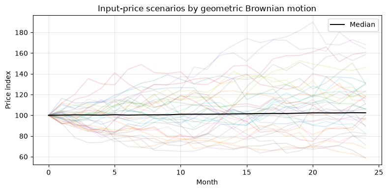
Reading the results

There is a difference between the median and upper quantile after 24 months, and a single price assumption alone overlooks upside risk. By calculating the profit and NPV for each route for each investment project, you can compare them with the probability of losing money. Because real prices have mean regression, jumps, and seasonality, mechanical extrapolation of past volatility is avoided.

No.078: Representing the Degradation Index of Mean Regression in Stochastic Differential Equations

Meaning in Practice

It handles indicators such as temperature and control deviations that return to the standard through control even if shaken by disturbances. You can evaluate deviation times more realistically than just random walks.

Approach to Analysis and Modeling

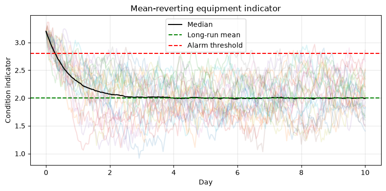
Discretize the Ornstein–Uhlenbeck process $dX_t=\theta(\mu-X_t)dt+\sigma dW_t$ using the Euler–Maruyama method. $\theta$ is the recovery speed, $\mu$ is the long-term average, and $\sigma$ is the disturbance strength. If the $\Delta t$ is too coarse, numerical errors increase, so verification of the indices is necessary.

Check with Python

n_paths, n_steps, dt = 3000, 240, 1/24
theta, long_mean, sigma_ou, x0 = 1.4, 2.0, 0.55, 3.2
ou = np.zeros((n_paths, n_steps+1)); ou[:,0] = x0
for k in range(n_steps):
    ou[:,k+1] = ou[:,k] + theta*(long_mean-ou[:,k])*dt + sigma_ou*np.sqrt(dt)*rng.normal(size=n_paths)
threshold = 2.8
exceed_hours = (ou[:,1:] > threshold).sum(axis=1)
print(f"Mean hours above threshold: {exceed_hours.mean():.2f}")
print(f"P(above threshold for >= 8 hours): {(exceed_hours >= 8).mean():.2%}")
fig, ax = plt.subplots()
time_ou = np.arange(n_steps+1)*dt
for p in ou[:25]: ax.plot(time_ou, p, alpha=.15)
ax.plot(time_ou, np.median(ou, axis=0), color="black", label="Median")
ax.axhline(long_mean, color="green", linestyle="--", label="Long-run mean")
ax.axhline(threshold, color="red", linestyle="--", label="Alarm threshold")
ax.set_title("Mean-reverting equipment indicator")
ax.set_xlabel("Day"); ax.set_ylabel("Condition indicator")
ax.grid(True, alpha=.3); ax.legend(); plt.tight_layout(); plt.show()

Mean hours above threshold: 10.48
P(above threshold for >= 8 hours): 58.40%

Reading the results

Even if the initial value is high, it returns to the average, but disturbances repeatedly cause threshold exceedances. Compared to single overruns, operational KPIs like “cumulative overruns of 8 hours or more” become more stable. Parameters should be estimated for each equipment and operating condition, and the independence and distribution of residuals must be checked.

No.079: Removing Sensor Noise with a Kalman Filter

Meaning in Practice

When true degradation cannot be directly measured, past estimates and new sensor values are integrated according to uncertainty. Compared to the raw moving average, the advantage is that you can clearly indicate the range of estimation error.

Approach to Analysis and Modeling

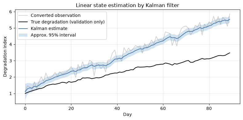
Assume the linear state space model $x_t=Ax_{t-1}+w_t$, $y_t=Hx_t+v_t$. From the variance of prediction and observational errors, calculate the Karman gain $K_t$ and give weight to the more reliable side. Here, we use degradation observations that convert vibrations linearly.

Check with Python

y_linear = (vibration - 1.2) / 0.85
A, H, Q, R = 1.0, 1.0, 0.045**2 + 0.01**2, (0.22/0.85)**2
x_est, cov = 0.8, 0.4
estimates, variances = [], []
for y in y_linear:
    x_pred = A*x_est + 0.025
    p_pred = A*cov*A + Q
    gain = p_pred*H/(H*p_pred*H + R)
    x_est = x_pred + gain*(y-H*x_pred)
    cov = (1-gain*H)*p_pred
    estimates.append(x_est); variances.append(cov)
estimates, variances = np.array(estimates), np.array(variances)
rmse_raw = np.sqrt(np.mean((y_linear-true_health)**2))
rmse_kf = np.sqrt(np.mean((estimates-true_health)**2))
print(f"Raw-observation RMSE : {rmse_raw:.3f}")
print(f"Kalman-filter RMSE   : {rmse_kf:.3f}")
fig, ax = plt.subplots()
ax.plot(t, y_linear, color="gray", alpha=.35, label="Converted observation")
ax.plot(t, true_health, color="black", label="True degradation (validation only)")
ax.plot(t, estimates, color="#4c78a8", label="Kalman estimate")
sd = np.sqrt(variances)
ax.fill_between(t, estimates-1.96*sd, estimates+1.96*sd, alpha=.2, label="Approx. 95% interval")
ax.set_title("Linear state estimation by Kalman filter")
ax.set_xlabel("Day"); ax.set_ylabel("Degradation index")
ax.grid(True, alpha=.3); ax.legend(); plt.tight_layout(); plt.show()

Raw-observation RMSE : 1.372
Kalman-filter RMSE   : 1.249

Reading the results

Filter estimation suppresses observational noise and allows for comparison of RMSE against true values. Rules can include uncertainty, such as inspecting if the 95% section exceeds the conservation standard. If linearity and normality are greatly disrupted, bias occurs, so the following particle filters are considered for nonlinear observations.

No.080: Estimating Nonlinear Equipment Conditions with Particle Filters

Meaning in Practice

When the observation relationship is nonlinear, such as the vibration value increasing quadratively with respect to the degree of degradation, the latent state is sequentially estimated. Because multiple possibilities can be held as particle groups, it can handle situations where distribution is distorted.

Approach to Analysis and Modeling

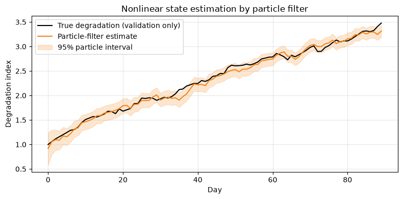
Particle filters approximate the state distribution with many particles $x_t^{(i)}$ and weights $w_t^{(i)}$. Repeat predictions, weight updates based on likelihoods, normalization, and resampling. The more particles you have, the more stable the approximation becomes, but the computational complexity also increases.

Check with Python

n_particles = 4000
pf_rng = np.random.default_rng(SEED+80)
particles = np.clip(pf_rng.normal(.8, .35, n_particles), 0, None)
pf_est, pf_low, pf_high, ess_history = [], [], [], []
for y in vibration:
    particles = np.clip(particles + 0.025 + pf_rng.normal(0, .045, n_particles), 0, None)
    predicted_y = 1.2 + .85*particles + .18*particles**2
    weights = np.exp(-.5*((y-predicted_y)/.22)**2)
    weights += 1e-300; weights /= weights.sum()
    pf_est.append(np.sum(weights*particles))
    order = np.argsort(particles); sorted_p = particles[order]; cum_w = np.cumsum(weights[order])
    pf_low.append(np.interp(.025, cum_w, sorted_p)); pf_high.append(np.interp(.975, cum_w, sorted_p))
    ess_history.append(1/np.sum(weights**2))
    positions = (pf_rng.random() + np.arange(n_particles))/n_particles
    indexes = np.searchsorted(np.cumsum(weights), positions)
    particles = particles[indexes]
pf_est, pf_low, pf_high = map(np.array, (pf_est, pf_low, pf_high))
print(f"Particle-filter RMSE: {np.sqrt(np.mean((pf_est-true_health)**2)):.3f}")
print(f"Mean effective sample size before resampling: {np.mean(ess_history):.0f}/{n_particles}")
fig, ax = plt.subplots()
ax.plot(t, true_health, color="black", label="True degradation (validation only)")
ax.plot(t, pf_est, color="#f58518", label="Particle-filter estimate")
ax.fill_between(t, pf_low, pf_high, color="#f58518", alpha=.2, label="95% particle interval")
ax.set_title("Nonlinear state estimation by particle filter")
ax.set_xlabel("Day"); ax.set_ylabel("Degradation index")
ax.grid(True, alpha=.3); ax.legend(); plt.tight_layout(); plt.show()

Particle-filter RMSE: 0.067
Mean effective sample size before resampling: 3199/4000

Reading the results

By directly using nonlinear vibration models, estimates and intervals close to true degradation can be obtained. The effective sample size is a diagnostic indicator for monitoring particle bias. During implementation, verify particle count, likelihood rate, and resampling methods, and evaluate “how many days in advance an alarm was triggered” based on known failure history.

Practical Implications Seen Through Target Exercise

1. Separate by state, number of cases, and continuous volume: For equipment conditions, the Markov chain is the starting point; for independent occurrences, the Poisson process is the starting point; for continuous fluctuations, the stochastic differential equation is the starting point.
2. Distinguishing between observed and true states: Sensor values are not regarded as the state itself; observation errors are clearly indicated using HMM, Karman filters, and particle filters.
3. Determined by distribution, not average: In addition to the expected number of failures, KPIs include inventory shortage probability, upper quantile, and interval estimation.
4. Increasing complexity step by step: Based on explainable simple models, it only advances when residuals and decision value improve.
5. Connecting models to costs: Convert probabilities into stoppage losses, inspection costs, inventory costs, and quality losses to compare measures.

What is necessary for practical implementation

• Standardize condition definitions, failure codes, time accuracy, and standards for recording replacement and repair
• Records of missing measurements, sensor replacements, downtime, and changes in operating conditions
• Separate training periods and future validation periods to prevent data leaks at the equipment and time level
• Evaluate not only accuracy but also alarm lead time, missed losses, and false alarm response man-hours
• Confirm parameter ranges and physical constraints with on-site knowledge
• Design from drift monitoring, regular reestimation, model approval, to standard operations after alerts

If you want to start small, narrow down to one critical equipment series and one decision (e.g., a detailed inspection within 7 days), and proceed with parallel evaluation alongside existing rules.

Conclusion

From No.071 to No.080, we implemented equipment condition transitions, long-term ratios, latent states, number of events, replacement cycles, continuous fluctuations, and sequential estimation. The value of stochastic processes lies not in definitive futures but in showing the possible range and probability, and in quantifying criteria for conservation, inventory, and investment decisions.

The first practical step is to clarify “which decisions you want to change, in advance, and by which loss criteria” rather than selecting models. Designing the minimum necessary state, observation, and temporal granularity according to that question makes it easier for analysis to translate into operational needs.

Consultations for Corporations

At Suri Kobo, we support the entire data preparation stage, including equipment maintenance, failure and demand simulation, condition estimation using sensor data, and designing decision-making KPIs in manufacturing. You can consult about designs that do not end with just PoC, but also consider on-site operation, evaluation, and renewal.

📩 Contact Us: surikobo.co.jp/contact
Please feel free to consult us first.