Deciphering the Manufacturing Floor Through the ‘Movement of Individuals’: 10 Agent-Based Simulation Practices

In this article, we treat equipment, workers, transport vehicles, and business partners as the main decision-making agents (agents), and examine how local actions affect the overall safety, delivery times, inventory, and profits of the entire factory, using ten items No.051 to No.060. We examine congestion, chain stoppages, and the penetration of improvement activities that are hard to see from averages alone, using reproducible fictional data and Python.

[!NOTE] This material is a notebook previously used by Surikoubo (or personally by the representative, Kazuyama), and has been reconstructed, edited, and published with the company’s permission. All data listed is fictional and has no relation whatsoever to real companies, factories, or figures.

Introduction: Practical Challenges in Manufacturing Covered in This Article

The target is a fictional factory that assembles a wide variety of parts. On site, there are workers with different skills, multiple AGVs, and business partners with varying delivery schedules and supply stability. The decisions we want to consider are: (1) safe flow lines, (2) transport rules, (3) supplier dispersion, (4) establishment of improvement behaviors, and (5) introduction of autonomous control.

Common situations on site

Even if the monthly average occupancy rate is reasonable, the aisles may become congested only after breaks. Even with order volumes that meet average demand, a single delay by one company can cause a line stoppage. Also, even when notifying standard tasks, the speed of penetration varies depending on the consultation relationship on site. If individual differences and interactions are eliminated and aggregated, these phenomena cannot be explained.

Why is this issue so difficult to judge?

If we $s_i(t)$ the state of Agent $i$, $a_i(t)$ actions, and $N_i(t)$ neighborhood, then the update conceptually

$s_i(t+1)=f_i\left(s_i(t),a_i(t),\{s_j(t):j\in N_i(t)\},\varepsilon_i(t)\right)$

It can be expressed as such. The overall KPI is $K(t)=g(s_1(t),\ldots,s_n(t))$, but since $f_i$ is nonlinear and neighborhoods change, simply examining an average single agent cannot estimate the overall result. ABM is not a predictive device, but an experimental device that compares “which assumptions and what results will occur.”

Overview of Exercise covered this time

No.	Theme	Judgment in the manufacturing industry
051	What is ABM?	Distinguishing between aggregation models and individual models
052	Agent Design	Definition of State, Behavior, and Rules
053	Crowd	Evacuation and Passageway Congestion Evaluation
054	traffic flow	AGV Density and Transport Capacity
055	Market	Impact of Price, Quality, and Delivery Times on Order Orders
056	Infectious diseases	Absence risk through contact
057	supply chain	Order chains and bullwhips
058	Organization	Promotion of Improvement Behaviors
059	Integration with Reinforcement Learning	Learning Transport Rules by Condition
060	Getting Started with Mesa	Standard Form of Model Implementation

Preparing the Python environment

The random number generator is unified to default_rng, and each experiment explicitly specifies the seed. Graphs are paired with comparable units and axes.

import sys
import numpy as np
import pandas as pd
import matplotlib
import matplotlib.pyplot as plt
from dataclasses import dataclass

try:
    import japanize_matplotlib  # Japanese Font Settings
except ImportError:
    pass

pd.set_option("display.precision", 2)
print(f"Python {sys.version.split()[0]}")
print(f"numpy {np.__version__} / pandas {pd.__version__} / matplotlib {matplotlib.__version__}")

Python 3.13.1
numpy 2.5.1 / pandas 3.0.3 / matplotlib 3.11.0

Creation of Fictional Data

Assign 30 workers skills, walking speed, readiness to improve, and assigned teams. This is not an individual evaluation, but an example of input for a model with individual differences. In practice, labor and management must agree on anonymization, granularity, and purpose of use.

rng = np.random.default_rng(1606)
n_workers = 30
workers = pd.DataFrame({
    "worker_id": [f"W{i:02d}" for i in range(1, n_workers + 1)],
    "team": rng.choice(list("ABC"), n_workers),
    "skill": np.clip(rng.normal(0.75, 0.12, n_workers), 0.4, 1.0),
    "walk_speed_m_s": np.clip(rng.normal(1.25, 0.15, n_workers), 0.8, 1.6),
    "improvement_receptivity": rng.beta(3, 2, n_workers),
})
workers.head()

	worker_id	team	skill	walk_speed_m_s	improvement_receptivity
0	W01	B	0.81	1.48	0.82
1	W02	A	0.64	1.32	0.79
2	W03	B	0.78	0.81	0.49
3	W04	B	0.73	1.46	0.53
4	W05	C	0.45	1.33	0.74

No.051: What is ABM?

Meaning in Practice

Leaving heterogeneity that disappears in aggregate data, we observe the process by which overall KPIs emerge from local rules. In factories, even with the same average processing capacity, stagnation can vary depending on skill imbalances and supportive behaviors.

Approach to Analysis and Modeling

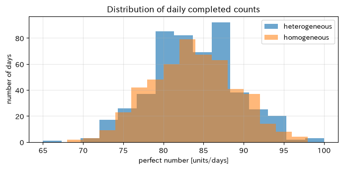
Each worker is given a skill, and successful processing is reproduced as a Bernoulli trial. We compare not only the averages of homogeneous and heterogeneous models, but also daily downside risks.

Check with Python

rng = np.random.default_rng(51)
days, jobs = 500, 120
hetero = np.array([(rng.random(jobs) < rng.choice(workers.skill, jobs)).sum() for _ in range(days)])
mean_skill = workers.skill.mean()
homogeneous = rng.binomial(jobs, mean_skill, days)
result_051 = pd.DataFrame({"model": ["heterogeneous worker", "average worker"], "average number of completed": [hetero.mean(), homogeneous.mean()], "5%point": [np.quantile(hetero,.05), np.quantile(homogeneous,.05)]})
display(result_051.round(1))
plt.figure(figsize=(7, 3.5)); plt.hist(hetero, bins=15, alpha=.65, label="heterogeneous"); plt.hist(homogeneous, bins=15, alpha=.55, label="homogeneous")
plt.title("Distribution of daily completed counts"); plt.xlabel("perfect number [units/days]"); plt.ylabel("number of days"); plt.grid(alpha=.3); plt.legend(); plt.tight_layout(); plt.show()

	model	average number of completed	5%point
0	heterogeneous worker	83.6	75.0
1	average worker	83.1	75.0

Reading the results

Even if the average number of completed items is close, differences in lower quantile points mean different margins required to guarantee delivery times. ABM’s value lies not in accurately calculating averages, but in placing the risks of heterogeneity in decision-making.

No.052: Agent Design

Meaning in Practice

The explainability of a model depends on who can define what to observe and how it operates in business terms. Increasing attributes is not necessarily better; only the differences necessary for decision-making are retained.

Approach to Analysis and Modeling

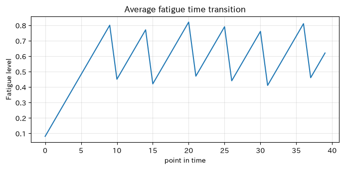
It represents workers in skill, fatigue, and available states, as well as actions such as working or resting. Fatigue is a simple state transition that lowers productivity and is recovered through breaks.

Check with Python

@dataclass
class WorkerAgent:
    skill: float
    fatigue: float = 0.0
    produced: int = 0
    def step(self, rng):
        if self.fatigue > 0.75:
            self.fatigue = max(0, self.fatigue - 0.35); return "Break"
        success = rng.random() < self.skill * (1 - 0.35*self.fatigue)
        self.produced += int(success); self.fatigue = min(1, self.fatigue + 0.08)
        return "Production"
rng = np.random.default_rng(52); agents = [WorkerAgent(s) for s in workers.skill[:8]]
records=[]
for t in range(40):
    for i,a in enumerate(agents): records.append((t,i,a.step(rng),a.fatigue,a.produced))
trace_052=pd.DataFrame(records,columns=["point in time","agent","action","fatigue","cumulative production"])
display(trace_052.groupby("action").size().rename("number of times").to_frame())
avg=trace_052.groupby("point in time").fatigue.mean(); plt.figure(figsize=(7,3.5)); plt.plot(avg.index,avg.values)
plt.title("Average fatigue time transition"); plt.xlabel("point in time"); plt.ylabel("Fatigue level"); plt.grid(alpha=.3); plt.tight_layout(); plt.show()

	number of times
action
Break	48
Production	272

Reading the results

You can see that the break rule periodically reduces fatigue. In practice, fatigue levels are not arbitrarily estimated; instead, break records, workload, and ergonomic rationales are used, and they are utilized for process design rather than personal monitoring.

No.053: Crowd Simulation

Meaning in Practice

During shifts or evacuations, if everyone chooses the shortest route, exits will get congested. Compare peak density with evacuation completion time and use it to make investment decisions regarding aisle width and guidance policies.

Approach to Analysis and Modeling

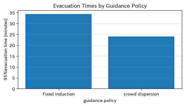
This is a simple model where workers are concentrated at two exits. We compare cases where each exit has its own processing capacity and concentrates 90% of the effort at the nearest exit versus when congestion is dispersed.

Check with Python

def evacuate(seed, adaptive, n=120):
    rng=np.random.default_rng(seed); queues=[0,0]; done=[]
    for _ in range(n):
        choice=int(np.argmin(queues)) if adaptive and rng.random()<.85 else int(rng.random()>.8)
        queues[choice]+=1; done.append(queues[choice]/[3.0,2.5][choice])
    return max(done), max(queues)
rows=[]
for policy in [False,True]:
    vals=[evacuate(s,policy) for s in range(300)]
    rows.append(["Fixed induction" if not policy else "crowd dispersion",np.mean(vals,0)[0],np.quantile(np.array(vals)[:,0],.95),np.mean(vals,0)[1]])
result_053=pd.DataFrame(rows,columns=["policy","Average Evacuation Time","95%evacuation time","Maximum Waiting Capacity"]); display(result_053.round(1))
plt.figure(figsize=(6,3.5)); plt.bar(result_053.policy,result_053["95%evacuation time"]); plt.title("Evacuation Times by Guidance Policy"); plt.xlabel("guidance policy"); plt.ylabel("95%evacuation time [minutes]"); plt.grid(axis="y",alpha=.3); plt.tight_layout(); plt.show()

	policy	Average Evacuation Time	95%evacuation time	Maximum Waiting Capacity
0	Fixed induction	32.0	34.3	96.0
1	crowd dispersion	23.9	24.0	60.2

Reading the results

If congestion dispersion reduces the score by 95%, the value of floor displays and digital signage can be quantified. However, safety design is not finalized solely for this model; priority is given to regulations, on-site training, and expert reviews.

No.054: Traffic Flow Simulation

Meaning in Practice

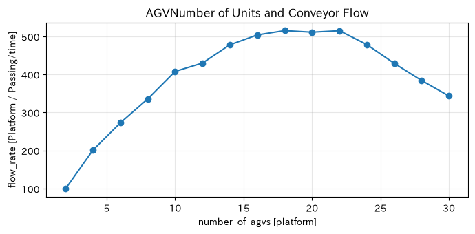
Increasing the number of AGVs does not necessarily mean the transport volume will increase proportionally. We see the limit effect of adding more vehicles, including speed reductions caused by intersection interference and following.

Approach to Analysis and Modeling

A basic diagram where the speed decreases by $v=v_0(1-k/k_{jam})$ for density $k$ is reproduced, leaving the speed differences for each AGV. The flow rate is $q=kv$.

Check with Python

rng=np.random.default_rng(54); rows=[]
for n in range(2,31,2):
    density=n/100
    speeds=np.clip(rng.normal(1.5*(1-density/.38),.06,n),.05,None)
    rows.append((n,speeds.mean(),density*speeds.mean()*3600))
result_054=pd.DataFrame(rows,columns=["number_of_agvs","average_speed_m_s","flow_rate_table_time"]); display(result_054.loc[result_054.flow_rate_table_time.nlargest(3).index].round(2))
plt.figure(figsize=(7,3.5)); plt.plot(result_054.number_of_agvs,result_054.flow_rate_table_time,marker="o"); plt.title("AGVNumber of Units and Conveyor Flow"); plt.xlabel("number_of_agvs [platform]"); plt.ylabel("flow_rate [Platform / Passing/time]"); plt.grid(alpha=.3); plt.tight_layout(); plt.show()

	AGVNumber of units	average_speed_m_s	flow_rate_table_time
8	18	0.80	515.30
10	22	0.65	515.08
9	20	0.71	511.15

Reading the results

Increasing the number of cars beyond the curve peak can have the opposite effect due to speed reduction. In actual implementation, intersection occupancy time, charging, breakdown, and priority control are added, and route separation is considered as a candidate not only for vehicle count but also for route separation.

No.055: Market Simulation

Meaning in Practice

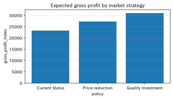
Orders in manufacturing vary not only by price but also by the composition of customer groups that respond to quality and delivery times. Compare on a customer-by-customer basis whether price reductions or quality investments are more effective for gross margins.

Approach to Analysis and Modeling

$U_i=-w_{p,i}p+w_{q,i}q-w_{l,i}l+\varepsilon_i$ the utility of the customer $i$, and orders are accepted only when utility is higher than competitors. Preferences vary for each customer.

Check with Python

rng=np.random.default_rng(55); n=1000
w=rng.dirichlet([3,4,2],n); competitor=-w[:,0]*100+w[:,1]*82-w[:,2]*8
scenarios={"Current Status":(102,85,7,35),"Price reduction":(96,85,7,29),"Quality Investment":(102,92,6,33)}; rows=[]
for name,(p,q,l,margin) in scenarios.items():
    utility=-w[:,0]*p+w[:,1]*q-w[:,2]*l+rng.normal(0,2,n)
    share=(utility>competitor).mean(); rows.append((name,share,share*n*margin))
result_055=pd.DataFrame(rows,columns=["policy","Order rate","gross_profit_index"]); display(result_055.round(2))
plt.figure(figsize=(6,3.5)); plt.bar(result_055.policy,result_055.gross_profit_index); plt.title("Expected gross profit by market strategy"); plt.xlabel("policy"); plt.ylabel("gross_profit_index"); plt.grid(axis="y",alpha=.3); plt.tight_layout(); plt.show()

	policy	Order rate	gross_profit_index
0	Current Status	0.66	23240.0
1	Price reduction	0.94	27202.0
2	Quality Investment	0.94	30954.0

Reading the results

The maximum order rate and maximum gross profit may not match. It is important to calibrate the weights by customer segment based on actual performance and confirm that the policy rankings remain robust even when competitive conditions are set.

No.056: Infectious Disease Simulation

Meaning in Practice

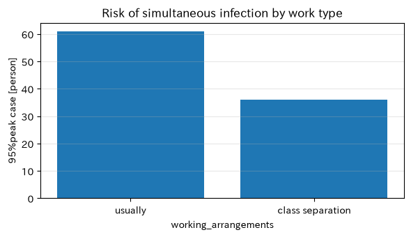
The spread of infection not only affects employee health but also leads to skill shortages and delayed deliveries due to simultaneous absenteeism. We evaluate the business continuity effects of measures to reduce inter-team contact.

Approach to Analysis and Modeling

An SIR-type individual model with susceptibility S, infection I, and recovery R. Each day, the probability of infection $1-(1-\beta)^c$ is calculated based on the number of contacts with infected individuals.

Check with Python

def outbreak(seed, split, n=80, days=35):
    rng=np.random.default_rng(seed); state=np.zeros(n,int); state[0]=1; age=np.zeros(n,int); peak=1
    for _ in range(days):
        inf=np.where(state==1)[0]; new=[]
        for i in np.where(state==0)[0]:
            contacts=sum((rng.random(len(inf)) < (0.035 if split else 0.07)))
            if rng.random()<1-(1-.12)**contacts:new.append(i)
        age[inf]+=1; state[np.array(new,int)]=1; state[(state==1)&(age>=6)]=2; peak=max(peak,(state==1).sum())
    return peak,(state==2).sum()
rows=[]
for split in [False,True]:
    a=np.array([outbreak(s,split) for s in range(400)])
    rows.append(("usually" if not split else "class separation",a[:,0].mean(),np.quantile(a[:,0],.95),a[:,1].mean()))
result_056=pd.DataFrame(rows,columns=["working_arrangements","Average peak infection","95%peak case","Average cumulative infections"]); display(result_056.round(1))
plt.figure(figsize=(6,3.5)); plt.bar(result_056.working_arrangements,result_056["95%peak case"]); plt.title("Risk of simultaneous infection by work type"); plt.xlabel("working_arrangements"); plt.ylabel("95%peak case [person]"); plt.grid(axis="y",alpha=.3); plt.tight_layout(); plt.show()

	working_arrangements	Average peak infection	95%peak case	Average cumulative infections
0	usually	52.7	61.0	77.1
1	class separation	20.1	36.0	46.0

Reading the results

Team separation can suppress peaks and reduce simultaneous absenteeism for critical skills. This is not a medical forecast. Actual measures follow public guidance and the advice of occupational physicians, limiting the model to considering the staffing capacity of BCPs.

No.057: Supply Chain Simulation

Meaning in Practice

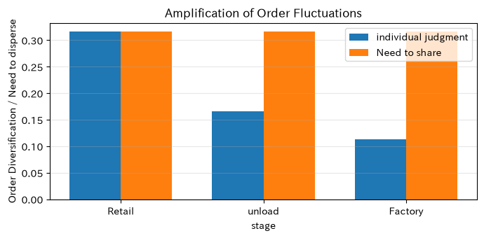
When each stage places orders based solely on their own inventory, even small fluctuations in demand are amplified upstream. Identify the trade-off between reducing stockouts and increasing inventory.

Approach to Analysis and Modeling

Retail, wholesale, and factory use an order-up-to rule to fill the gap with target inventory. Compare the distribution of order volumes, i.e., the bullwhip ratio, depending on whether information is shared.

Check with Python

def chain(seed, shared, T=100):
    rng=np.random.default_rng(seed); demand=np.maximum(0,rng.normal(20,3,T)); inv=np.array([40.,40.,40.]); orders=[]
    prev=np.array([20.,20.,20.])
    for t,d in enumerate(demand):
        signal=np.repeat(d,3) if shared else np.r_[d,prev[:2]]
        order=np.maximum(0,20+.55*(40-inv)+.45*(signal-20)); inv+=prev-order; prev=order; orders.append(order)
    return demand,np.array(orders)
rows=[]
for shared in [False,True]:
    d,o=chain(57,shared); rows.append(("individual judgment" if not shared else "Need to share",*(o.var(0)/d.var())))
result_057=pd.DataFrame(rows,columns=["Method","Retail bullwhip ratio","Wholesale Bullwhip Ratio","Factory Bullwhip Ratio"]); display(result_057.round(2))
plt.figure(figsize=(7,3.5)); x=np.arange(3); plt.bar(x-.18,result_057.iloc[0,1:],.36,label="individual judgment"); plt.bar(x+.18,result_057.iloc[1,1:],.36,label="Need to share"); plt.xticks(x,["Retail","unload","Factory"]); plt.title("Amplification of Order Fluctuations"); plt.xlabel("stage"); plt.ylabel("Order Diversification / Need to disperse"); plt.grid(axis="y",alpha=.3); plt.legend(); plt.tight_layout(); plt.show()

	Method	Retail bullwhip ratio	Wholesale Bullwhip Ratio	Factory Bullwhip Ratio
0	individual judgment	0.32	0.17	0.11
1	Need to share	0.32	0.32	0.32

Reading the results

If demand sharing reduces upstream variance, the benefits of EDI and common dashboards can be converted into inventory and capacity planning. Lead time, minimum lot, and supply constraints are added before deciding to change the contract.

No.058: Organizational Simulation

Meaning in Practice

Even if the content of improvement measures is correct, they may not take root depending on consultation or managerial intervention. We will consider how to select trainees and assign on-site leaders.

Approach to Analysis and Modeling

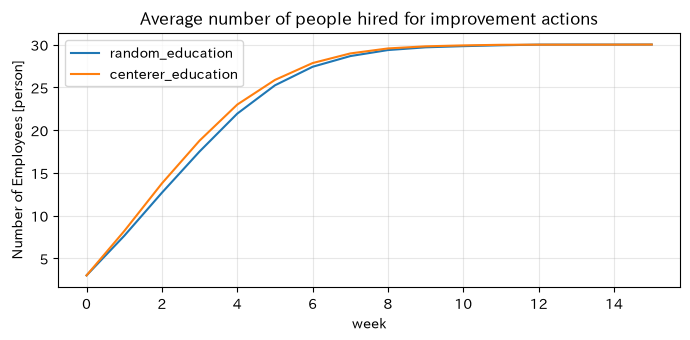
Within the network among workers, the probability of hiring is determined based on the ratio of hired colleagues and the individual’s acceptance. Random initial education is compared with education for people with many connections.

Check with Python

rng=np.random.default_rng(58); n=30; A=(rng.random((n,n))<.12).astype(int); A=np.triu(A,1); A=A+A.T; degree=A.sum(1)
def diffuse(seed, targeted):
    rng=np.random.default_rng(seed); adopted=np.zeros(n,bool); initial=np.argsort(degree)[-3:] if targeted else rng.choice(n,3,False); adopted[initial]=True; hist=[adopted.sum()]
    for _ in range(15):
        ratio=(A@adopted)/np.maximum(degree,1); p=np.clip(.03+.55*ratio+workers.improvement_receptivity.to_numpy()*.12,0,1)
        adopted |= rng.random(n)<p; hist.append(adopted.sum())
    return hist
h_random=np.mean([diffuse(s,False) for s in range(200)],0); h_target=np.mean([diffuse(s,True) for s in range(200)],0)
result_058=pd.DataFrame({"week":range(16),"random_education":h_random,"centerer_education":h_target}); display(result_058.tail().round(1))
plt.figure(figsize=(7,3.5)); plt.plot(result_058.week,result_058.random_education,label="random_education"); plt.plot(result_058.week,result_058.centerer_education,label="centerer_education"); plt.title("Average number of people hired for improvement actions"); plt.xlabel("week"); plt.ylabel("Number of Employees [person]"); plt.grid(alpha=.3); plt.legend(); plt.tight_layout(); plt.show()

	week	random_education	centerer_education
11	11	29.9	30.0
12	12	30.0	30.0
13	13	30.0	30.0
14	14	30.0	30.0
15	15	30.0	30.0

Reading the results

Leading education to the core may accelerate early penetration. However, do not apply network analysis to personnel evaluations; instead, under the individual’s consent and privacy protection, design the official support role.

No.059: Integration with Reinforcement Learning

Meaning in Practice

With fixed rules, it can be difficult to make transport decisions suitable for both normal and busy conditions. It uses the simulator as a safe trial environment to learn state-specific rules.

Approach to Analysis and Modeling

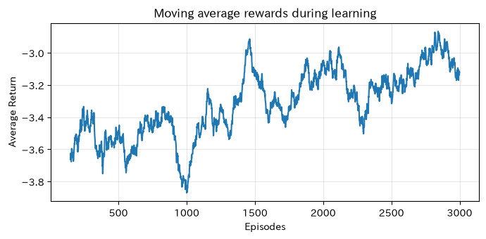
This is a minimal example of Q-learning where queues are considered status, normal transport and detour are actions, and delays and detour costs are negative rewards. The update formula is $Q\leftarrow Q+\alpha[r+\gamma\max Q'-Q]$.

Check with Python

rng=np.random.default_rng(59); Q=np.zeros((3,2)); alpha=.12; gamma=.9; eps=.15; rewards=[]
for ep in range(3000):
    s=rng.integers(0,3); a=rng.integers(0,2) if rng.random()<eps else np.argmax(Q[s]); congestion=[1,4,9][s]
    delay=(congestion+rng.normal(0,.7)) if a==0 else (3.2+rng.normal(0,.4)); r=-delay-(.8 if a==1 else 0)
    ns=min(2,max(0,s+rng.choice([-1,0,1],p=[.2,.6,.2]))); Q[s,a]+=alpha*(r+gamma*Q[ns].max()-Q[s,a]); rewards.append(r)
policy=pd.DataFrame({"congestion condition":["low","middle","high"],"Selective behavior":np.where(Q.argmax(1)==0,"Normal route","detour"),"usuallyQ":Q[:,0],"detourQ":Q[:,1]}); display(policy.round(2))
roll=pd.Series(rewards).rolling(150).mean(); plt.figure(figsize=(7,3.5)); plt.plot(roll); plt.title("Moving average rewards during learning"); plt.xlabel("Episodes"); plt.ylabel("Average Return"); plt.grid(alpha=.3); plt.tight_layout(); plt.show()

	congestion condition	Selective behavior	usuallyQ	detourQ
0	low	Normal route	-23.11	-25.20
1	middle	detour	-32.70	-30.13
2	high	detour	-39.13	-33.02

Reading the results

If a policy is obtained to bypass only during peak congestion, it can be verified as a conditional branch. It provides safety layers that do not directly connect to production equipment, do not tolerate constraint violations, offline evaluation, manual switching, and monitoring KPIs.

No.060: Introduction to Mesa

Meaning in Practice

To continue using ABM, it is necessary to implement separate agents, models, schedulers, and data collection. Mesa is a Python framework that provides this structure.

Approach to Analysis and Modeling

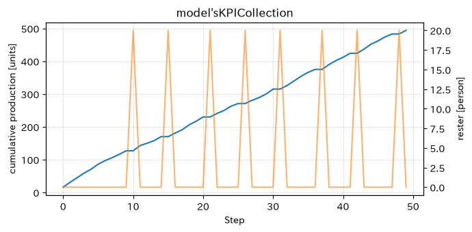
On a MiniModel that operates without additional dependencies, we implement step and data collection based on the same concept as Mesa. In actual cases, it is replaced by MESA’s Agent, Model, and DataCollector.

Check with Python

class MiniModel:
    def __init__(self, seed=60, n=20):
        self.rng=np.random.default_rng(seed); self.agents=[WorkerAgent(float(s)) for s in workers.skill[:n]]; self.history=[]
    def step(self):
        actions=[a.step(self.rng) for a in self.agents]
        self.history.append({"step":len(self.history),"total_output":sum(a.produced for a in self.agents),"resting":actions.count("Break")})
model=MiniModel()
for _ in range(50): model.step()
result_060=pd.DataFrame(model.history); display(result_060.tail())
fig,ax1=plt.subplots(figsize=(7,3.5)); ax1.plot(result_060.step,result_060.total_output,label="cumulative production"); ax1.set_xlabel("Step"); ax1.set_ylabel("cumulative production [units]"); ax2=ax1.twinx(); ax2.plot(result_060.step,result_060.resting,color="tab:orange",alpha=.6,label="rester"); ax2.set_ylabel("rester [person]"); ax1.set_title("model'sKPICollection"); ax1.grid(alpha=.3); fig.tight_layout(); plt.show()

	step	total_output	resting
45	45	462	0
46	46	474	0
47	47	483	0
48	48	483	20
49	49	494	0

Reading the results

Separating model structure from KPI collection makes rule changes and validation easier. We design operational processes that include model specifications, SEED management, unit testing, sensitivity analysis, and calibration against actual results, rather than simply adopting MESA itself.

Practical Implications Seen Through Target Exercise

What all 10 have in common is that they clearly indicate “variation, contact, and local judgment” rather than the average. ABM allows you to compare measures such as increasing fleets, separating teams, sharing information, and selecting training targets before deploying them to the field. On the other hand, the result is the consequence of assumptions. Rather than a single prediction value, you should report the distribution of multiple seeds, the lower and upper quantiles, and the boundaries where the order of the initiative changes.

What is necessary for practical implementation

1. Defining decision-making in advance: Decide by what month and how much the misjudgment costs to take.
2. Agreeing on boundaries and granularity: Prepare the specification document for processes, time units, subjects, conditions, actions, and external conditions.
3. Separate Proofreading from Validation: Parameters are matched during certain periods, and reproducibility is checked during different periods and shifts.
4. Conduct sensitivity analysis: Specifies uncertain inputs such as contact rate or processing power, and the conditions under which the conclusion is reversed.
5. Incorporating on-site reviews: Workers and managers check for exceptions, tacit knowledge, and safety constraints not found in the model.
6. Determine operational responsibilities: Define criteria for data updates, version management, approvals, monitoring, and decommissioning.

Conclusion

No.051–060 links the basics of ABM to crowds, traffic, markets, infections, supply chains, organization, reinforcement learning, and implementation structures in manufacturing decision-making. Starting with a small, explainable model and gradually refining it while learning from track record gaps helps balance ROI and on-site trust.

Consultations for Corporations

At Suri Kobo, we support everything from problem organization to model design, PoC, and on-site operations, covering areas such as in-factory logistics, production and inventory, supply chain, and personnel allocation. You can consult with us from the stage of “Not sure if the data is sufficient” or “Which is better, commercial tools or in-house ones?”

📩 Contact Us: surikobo.co.jp/contact Please feel free to consult us first.