100本ノック / 数理モデリング / 数理モデリング100本ノック

欠品・在庫・段取り・能力を同時に考える：多品種交換部品で学ぶ在庫・生産のモデル化

2020-02-07

欠品・在庫・段取り・能力を同時に考える

多品種交換部品で学ぶ在庫・生産のモデル化 No.041〜No.050

本記事では、架空の産業機器向け交換部品3製品を題材に、在庫残高、発注点、安全在庫、欠品費、保管費、発注ロット、生産能力、段取り、リードタイム、多品種生産計画を一続きでモデル化します。

目的は在庫を単純に減らすことでも、欠品を完全になくすことでもありません。顧客サービス、運転資金、段取り負荷、設備能力のトレードオフを数値で比較し、実行可能な方針を選ぶことです。

[!NOTE] 本資料は、数理工房 (もしくは代表である和山個人) が過去に企業研修において使用した notebook を企業様の許可を得て再構成・編集のうえ公開しています。掲載データはすべて架空のものであり、実在する企業・工場・数値とは一切関係ありません。

はじめに：この記事で扱う製造業の実務課題

架空の部品工場では、交換部品A・B・Cを共通ラインで生産しています。Aは需要量が多く、Cは需要量が少ない一方で欠品時の顧客影響が大きい製品です。調達・生産リードタイムは製品ごとに異なり、ときどき遅延します。

生産管理は欠品を避けるため在庫を増やしたい一方、経理は在庫金額を抑えたいと考えています。小ロット化すれば平均在庫は減りますが、段取り回数と停止時間が増えます。需要増に対しては、設備時間と材料の制約も確認しなければなりません。

今回は180日分の架空需要を使い、在庫方程式から多品種生産計画、モデル評価まで段階的に整理します。

現場でよくある状況

月初在庫と入荷・出荷の関係が合わず、在庫差異の原因が追えない
発注点が担当者の経験値で、需要変動やリードタイムを反映していない
安全在庫を一律○日分とし、製品ごとの欠品影響を区別していない
在庫削減額だけを追い、欠品損失や緊急対応費を集計していない
小ロット化で在庫は減ったが、段取り増加で能力不足になった
製品別計画は成立していても、共通設備・材料を合計すると制約を超える
方針評価が平均在庫だけで、充足率・費用・安定性を比較していない

在庫と生産は別々の問題ではありません。発注量、段取り、能力、リードタイムが在庫状態を通じて相互に影響します。

なぜこの問題は判断が難しいのか

在庫を増やせば欠品は減りやすくなりますが、保管費、資金拘束、陳腐化が増えます。ロットを大きくすれば発注・段取り回数は減りますが、平均在庫が増えます。設備稼働時間には上限があり、重要度の異なる複数製品へ能力を配分する必要があります。

さらに、需要とリードタイムは確定値ではありません。平均需要だけで発注点を作ると、需要急増や入荷遅延を吸収できません。そのため、状態方程式、確率的な安全在庫、費用関数、能力制約、評価KPIを組み合わせます。

今回扱うノックの全体像

No.	テーマ	実務での判断
041	在庫残高	入荷・需要・欠品で在庫がどう変わるか
042	発注点	いつ補充を開始するか
043	安全在庫	需要・納期変動を何個吸収するか
044	欠品費と保管費	サービス水準をどこまで上げるか
045	発注ロット	1回に何個補充するか
046	生産能力制約	需要計画が設備時間内に収まるか
047	段取り替え	小ロット化の代償をどう評価するか
048	リードタイム	納期短縮が在庫へどう効くか
049	多品種生産計画	限られた能力をどの製品へ配分するか
050	評価指標	費用・在庫・欠品をどう総合比較するか

No.041〜050は、状態の記録、単品方針の設計、共通資源の配分、総合評価という流れです。

Python 環境の準備

外部データは使いません。NumPyで乱数シードを固定し、SciPyの正規分布と線形計画、pandas、matplotlibを使います。

%matplotlib inline
%config InlineBackend.figure_format = 'svg'

import platform
import sys

import matplotlib
import matplotlib.pyplot as plt
from matplotlib import font_manager
import numpy as np
import pandas as pd
import scipy
from scipy.optimize import linprog
from scipy.stats import norm
from IPython.display import display

SEED = 42
rng = np.random.default_rng(SEED)
available_fonts = {font.name for font in font_manager.fontManager.ttflist}
plot_font = next((f for f in ["Hiragino Sans", "Yu Gothic", "Noto Sans CJK JP"] if f in available_fonts), "sans-serif")
plt.rcParams["font.family"] = plot_font
plt.rcParams["axes.unicode_minus"] = False
plt.rcParams["figure.figsize"] = (9, 4.8)

print(f"Python     : {sys.version.split()[0]}")
print(f"NumPy      : {np.__version__}")
print(f"pandas     : {pd.__version__}")
print(f"SciPy      : {scipy.__version__}")
print(f"matplotlib : {matplotlib.__version__}")
print(f"plot font  : {plot_font}")
print(f"platform   : {platform.platform()}")
print(f"random seed: {SEED}")

Python     : 3.13.1
NumPy      : 2.5.1
pandas     : 3.0.3
SciPy      : 1.18.0
matplotlib : 3.11.0
plot font  : Hiragino Sans
platform   : macOS-26.3-arm64-arm-64bit-Mach-O
random seed: 42

架空データの作成

製品A・B・Cについて180日の日次需要を生成します。製品ごとに平均需要、標準リードタイム、保管費、欠品費、発注費、単価、加工時間、段取り時間が異なります。

現行方針は安全係数 $z=0.5$ の発注点と固定ロットです。5回に1回の補充で3日の遅延を発生させ、需要急増と納期変動による欠品を再現します。

dates = pd.date_range("2025-01-01", periods=180, freq="D")
products = pd.DataFrame({
    "product": ["A", "B", "C"],
    "base_daily_demand": [110, 74, 42],
    "standard_lead_days": [5, 8, 12],
    "holding_cost_day": [5, 8, 12],
    "shortage_cost_unit": [1_000, 1_600, 2_500],
    "order_cost": [50_000, 65_000, 80_000],
    "unit_cost": [3_500, 5_200, 8_000],
    "current_order_qty": [1_400, 1_000, 700],
    "cycle_minutes": [3.0, 4.5, 7.0],
    "setup_hours": [3.0, 4.0, 5.0],
    "setup_cost": [80_000, 110_000, 150_000],
    "margin": [1_400, 2_200, 3_400],
    "material_kg": [1.2, 1.8, 2.6],
})

demand_rows = []
for day_no, date in enumerate(dates):
    weekday_factor = 0.48 if date.dayofweek >= 5 else 1.0
    seasonal = 1 + 0.12 * np.sin(2 * np.pi * (day_no - 35) / 180)
    spike = 1.45 if rng.random() < 0.045 else 1.0
    for spec in products.itertuples(index=False):
        expected = spec.base_daily_demand * weekday_factor * seasonal * spike
        demand_rows.append({
            "date": date,
            "day_no": day_no,
            "product": spec.product,
            "expected_demand": expected,
            "demand_units": rng.poisson(max(1, expected)),
        })

demand = pd.DataFrame(demand_rows).merge(products, on="product", how="left")

history = []
for product, group in demand.groupby("product", sort=False):
    group = group.sort_values("date").reset_index(drop=True)
    spec = products.set_index("product").loc[product]
    mu, sigma = group["demand_units"].mean(), group["demand_units"].std(ddof=1)
    reorder_point = int(round(mu * spec["standard_lead_days"] + 0.5 * sigma * np.sqrt(spec["standard_lead_days"])))
    order_qty = int(spec["current_order_qty"])
    arrivals = np.zeros(len(group) + 30, dtype=int)
    on_hand = reorder_point + order_qty
    order_count = 0
    for i, row in group.iterrows():
        arrival = int(arrivals[i])
        begin = on_hand
        on_hand += arrival
        sales = min(on_hand, int(row["demand_units"]))
        shortage = int(row["demand_units"]) - sales
        on_hand -= sales
        inventory_position = on_hand + int(arrivals[i + 1:].sum())
        placed = 0
        if inventory_position <= reorder_point:
            placed = order_qty
            order_count += 1
            delay = 3 if order_count % 5 == 0 else 0
            arrivals[i + int(spec["standard_lead_days"]) + delay] += placed
        history.append({
            **row.to_dict(), "begin_inventory": begin, "arrival_units": arrival,
            "sales_units": sales, "shortage_units": shortage,
            "ending_inventory": on_hand, "order_units": placed,
            "current_reorder_point": reorder_point,
        })

inventory_data = pd.DataFrame(history)
print(f"レコード数: {len(inventory_data):,}行（180日 × 3製品）")
display(inventory_data.head(9).style.format({"expected_demand": "{:.1f}"}))

レコード数: 540行（180日 × 3製品）

	date	day_no	product	expected_demand	demand_units	base_daily_demand	standard_lead_days	holding_cost_day	shortage_cost_unit	order_cost	unit_cost	current_order_qty	cycle_minutes	setup_hours	setup_cost	margin	material_kg	begin_inventory	sales_units	ending_inventory	current_reorder_point
0	2025-01-01 00:00:00	0	A	97.6	96	110	5	5	1000	50000	3500	1400	3.000000	3.000000	80000	1400	1.200000	1914	96	1818	514
1	2025-01-02 00:00:00	1	A	97.8	94	110	5	5	1000	50000	3500	1400	3.000000	3.000000	80000	1400	1.200000	1818	94	1724	514
2	2025-01-03 00:00:00	2	A	97.9	79	110	5	5	1000	50000	3500	1400	3.000000	3.000000	80000	1400	1.200000	1724	79	1645	514
3	2025-01-04 00:00:00	3	A	47.1	53	110	5	5	1000	50000	3500	1400	3.000000	3.000000	80000	1400	1.200000	1645	53	1592	514
4	2025-01-05 00:00:00	4	A	47.2	67	110	5	5	1000	50000	3500	1400	3.000000	3.000000	80000	1400	1.200000	1592	67	1525	514
5	2025-01-06 00:00:00	5	A	98.6	90	110	5	5	1000	50000	3500	1400	3.000000	3.000000	80000	1400	1.200000	1525	90	1435	514
6	2025-01-07 00:00:00	6	A	98.8	109	110	5	5	1000	50000	3500	1400	3.000000	3.000000	80000	1400	1.200000	1435	109	1326	514
7	2025-01-08 00:00:00	7	A	143.6	154	110	5	5	1000	50000	3500	1400	3.000000	3.000000	80000	1400	1.200000	1326	154	1172	514
8	2025-01-09 00:00:00	8	A	99.3	85	110	5	5	1000	50000	3500	1400	3.000000	3.000000	80000	1400	1.200000	1172	85	1087	514

overview = inventory_data.groupby("product", as_index=False).agg(
    需要=("demand_units", "sum"), 販売=("sales_units", "sum"),
    欠品=("shortage_units", "sum"), 平均在庫=("ending_inventory", "mean"),
    欠品日=("shortage_units", lambda x: (x > 0).sum()),
    発注回数=("order_units", lambda x: (x > 0).sum()),
)
overview["需要充足率"] = overview["販売"] / overview["需要"]
display(overview.style.format({"平均在庫": "{:,.1f}", "需要充足率": "{:.2%}"}))

fig, axes = plt.subplots(1, 2, figsize=(11, 4.2))
for product, group in inventory_data.groupby("product"):
    axes[0].plot(group["date"], group["ending_inventory"], linewidth=1, label=product)
axes[0].set_title("製品別の日次期末在庫")
axes[0].set_xlabel("日付")
axes[0].set_ylabel("期末在庫（個）")
axes[0].grid(True, alpha=0.3)
axes[0].legend(title="製品")
axes[1].bar(overview["product"], overview["需要充足率"] * 100, color="#2c7fb8")
axes[1].set_title("現行方針の需要充足率")
axes[1].set_xlabel("製品")
axes[1].set_ylabel("需要充足率（%）")
axes[1].grid(True, axis="y", alpha=0.3)
plt.tight_layout()
plt.show()
print(f"全製品の欠品合計: {inventory_data['shortage_units'].sum():,}個")

	product	需要	販売	欠品	平均在庫	欠品日	発注回数	需要充足率
0	A	17250	16558	692	751.3	7	11	95.99%
1	B	11620	11210	410	550.7	7	11	96.47%
2	C	6552	6354	198	407.6	7	9	96.98%

$svg$

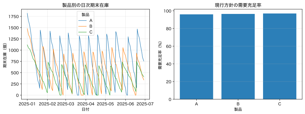
全製品の欠品合計: 1,300個

No.041：在庫残高の変化を数式で表現する

実務での意味

在庫は前日の状態を引き継ぐため、入荷・販売・欠品を時系列で整合させる必要があります。在庫方程式は帳簿差異の確認とシミュレーションの土台です。

分析・モデル化の考え方

I_t^{\mathrm{end}}=I_t^{\mathrm{begin}}+R_t-S_t

S_t=\min(D_t,I_t^{\mathrm{begin}}+R_t),\qquad U_t=D_t-S_t

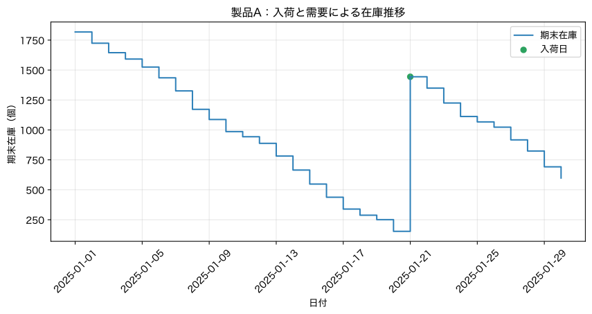
$R_t$ は入荷、 $S_t$ は販売、 $U_t$ は欠品です。失注型として欠品を翌日に持ち越しません。受注残型ならバックオーダー状態を追加します。

Pythonで確認する

balance = inventory_data.query("product == 'A'").head(30).copy()
balance["計算期末在庫"] = balance["begin_inventory"] + balance["arrival_units"] - balance["sales_units"]
balance["在庫差異"] = balance["計算期末在庫"] - balance["ending_inventory"]
display(balance[[
    "date", "begin_inventory", "arrival_units", "demand_units", "sales_units",
    "shortage_units", "ending_inventory", "在庫差異"
]].style.format({"date": "{:%m-%d}"}))

fig, ax = plt.subplots()
ax.step(balance["date"], balance["ending_inventory"], where="post", label="期末在庫", color="#2c7fb8")
ax.scatter(balance.loc[balance["arrival_units"] > 0, "date"], balance.loc[balance["arrival_units"] > 0, "ending_inventory"], color="#2ca25f", label="入荷日")
ax.set_title("製品A：入荷と需要による在庫推移")
ax.set_xlabel("日付")
ax.set_ylabel("期末在庫（個）")
ax.grid(True, alpha=0.3)
ax.legend()
plt.xticks(rotation=45)
plt.tight_layout()
plt.show()
print(f"在庫方程式の最大差異: {balance['在庫差異'].abs().max()}個")

	date	begin_inventory	arrival_units	demand_units	sales_units	ending_inventory
0	01-01	1914	0	96	96	1818
1	01-02	1818	0	94	94	1724
2	01-03	1724	0	79	79	1645
3	01-04	1645	0	53	53	1592
4	01-05	1592	0	67	67	1525
5	01-06	1525	0	90	90	1435
6	01-07	1435	0	109	109	1326
7	01-08	1326	0	154	154	1172
8	01-09	1172	0	85	85	1087
9	01-10	1087	0	101	101	986
10	01-11	986	0	43	43	943
11	01-12	943	0	55	55	888
12	01-13	888	0	106	106	782
13	01-14	782	0	117	117	665
14	01-15	665	0	117	117	548
15	01-16	548	0	110	110	438
16	01-17	438	0	99	99	339
17	01-18	339	0	51	51	288
18	01-19	288	0	37	37	251
19	01-20	251	0	98	98	153
20	01-21	153	1400	109	109	1444
21	01-22	1444	0	95	95	1349
22	01-23	1349	0	124	124	1225
23	01-24	1225	0	113	113	1112
24	01-25	1112	0	45	45	1067
25	01-26	1067	0	44	44	1023
26	01-27	1023	0	106	106	917
27	01-28	917	0	93	93	824
28	01-29	824	0	132	132	692
29	01-30	692	0	94	94	598

$svg$

在庫方程式の最大差異: 0個

結果の読み取り

需要で在庫が減り、入荷日に段階的に増える鋸歯状の動きが確認できます。在庫差異が0なので、入出庫と期末在庫が整合しています。

実務では検収時点、引当在庫、不良保留、仕掛品、棚卸修正を区別します。利用可能在庫と会計在庫を混同しないことが重要です。

No.042：発注点をモデル化する

実務での意味

発注点は、手元在庫と発注残を合わせた在庫ポジションが何個になったら補充するかを決めます。遅すぎれば欠品、早すぎれば在庫増になります。

分析・モデル化の考え方

R=\mu_D L+SS

$\mu_D L$ はリードタイム中の平均需要、 $SS$ は安全在庫です。判断には手元在庫ではなく、発注残と受注残を含む在庫ポジションを使います。

Pythonで確認する

reorder_rows = []
for product, group in inventory_data.groupby("product"):
    spec = products.set_index("product").loc[product]
    mu = group["demand_units"].mean()
    sigma = group["demand_units"].std(ddof=1)
    lead = spec["standard_lead_days"]
    safety_95 = norm.ppf(0.95) * sigma * np.sqrt(lead)
    reorder_rows.append({
        "製品": product, "平均日次需要": mu, "標準LT_日": lead,
        "LT平均需要": mu * lead, "95%安全在庫": safety_95,
        "推奨発注点": mu * lead + safety_95,
        "現行発注点": group["current_reorder_point"].iloc[0],
    })
reorder_table = pd.DataFrame(reorder_rows)
display(reorder_table.style.format({
    "平均日次需要": "{:.1f}", "LT平均需要": "{:.1f}",
    "95%安全在庫": "{:.1f}", "推奨発注点": "{:.0f}", "現行発注点": "{:.0f}"
}))

	製品	平均日次需要	標準LT_日	LT平均需要	95%安全在庫	推奨発注点	現行発注点
0	A	95.8	5.000000	479.2	112.9	592	514
1	B	64.6	8.000000	516.4	104.1	621	548
2	C	36.4	12.000000	436.8	75.8	513	460

結果の読み取り

現行発注点は安全係数0.5、推奨例は95%サービス水準のため、後者が高くなります。発注点を上げれば遅延耐性は増えますが、平均在庫も増えます。

発注点は需要予測とリードタイムの更新に合わせて見直します。季節性が強い製品には固定値ではなく時期別発注点を使います。

No.043：安全在庫をモデル化する

実務での意味

安全在庫は、平均需要を超える注文と平均を超える納期を吸収するバッファです。製品重要度に応じて目標サービス水準を変えます。

分析・モデル化の考え方

需要とリードタイムがともに変動するとき、近似標準偏差を、

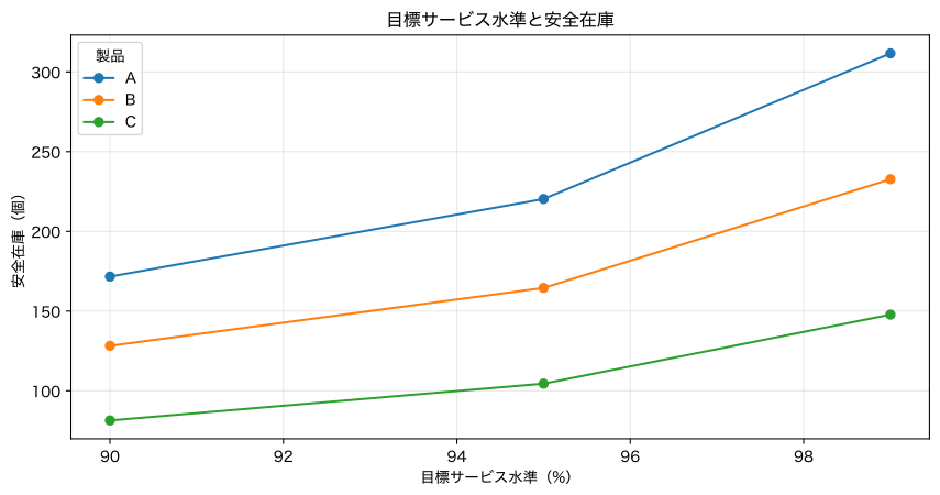
\sigma_{DL}=\sqrt{L\sigma_D^2+\mu_D^2\sigma_L^2}

とし、安全在庫を $SS=z\sigma_{DL}$ とします。 $z$ はサービス水準に対応する標準正規分布の分位点です。

Pythonで確認する

service_levels = [0.90, 0.95, 0.99]
rows = []
lead_sigma = 1.2
for product, group in inventory_data.groupby("product"):
    spec = products.set_index("product").loc[product]
    mu, sigma = group["demand_units"].mean(), group["demand_units"].std(ddof=1)
    sigma_lead_demand = np.sqrt(spec["standard_lead_days"] * sigma**2 + mu**2 * lead_sigma**2)
    for level in service_levels:
        z = norm.ppf(level)
        rows.append({"製品": product, "サービス水準": level, "z": z, "安全在庫": z * sigma_lead_demand})
safety_table = pd.DataFrame(rows)
display(safety_table.pivot(index="製品", columns="サービス水準", values="安全在庫").style.format("{:.0f}個"))

fig, ax = plt.subplots()
for product, group in safety_table.groupby("製品"):
    ax.plot(group["サービス水準"] * 100, group["安全在庫"], marker="o", label=product)
ax.set_title("目標サービス水準と安全在庫")
ax.set_xlabel("目標サービス水準（%）")
ax.set_ylabel("安全在庫（個）")
ax.grid(True, alpha=0.3)
ax.legend(title="製品")
plt.tight_layout()
plt.show()

サービス水準	0.900000	0.950000	0.990000
製品
A	172個	220個	312個
B	128個	165個	233個
C	81個	104個	148個

$svg$

結果の読み取り

99%へ近づくほど必要安全在庫が増えます。需要量、需要変動、リードタイムが大きい製品ほどバッファが必要です。

安全在庫は欠品をゼロにする保証ではありません。需要分布の歪み、連続欠品、供給停止を別シナリオで確認し、重要顧客向け部品は高い水準を設定します。

No.044：欠品コストと保管コストをモデル化する

実務での意味

安全在庫を増やすと保管費は増え、欠品費は減ります。両方を同じ費用尺度で比較すると、経済的なサービス水準を検討できます。

分析・モデル化の考え方

C(z)=h\sum_t I_t+c_s\sum_t U_t+K\times\text{発注回数}

$h$ は1個1日当たり保管費、 $c_s$ は欠品1個当たり損失、 $K$ は発注費です。欠品費には失注粗利、緊急輸送、顧客影響を含めます。

Pythonで確認する

def simulate_product(product, z, order_qty=None, lead_override=None):
    group = demand.query("product == @product").sort_values("date").reset_index(drop=True)
    spec = products.set_index("product").loc[product]
    mu, sigma = group["demand_units"].mean(), group["demand_units"].std(ddof=1)
    lead = int(lead_override or spec["standard_lead_days"])
    sigma_lt = np.sqrt(lead * sigma**2 + mu**2 * 1.2**2)
    rop = mu * lead + z * sigma_lt
    qty = float(order_qty or spec["current_order_qty"])
    arrivals = np.zeros(len(group) + 40)
    on_hand, lost, orders = rop + qty, 0.0, 0
    inv_history = []
    for i, d in enumerate(group["demand_units"].to_numpy()):
        on_hand += arrivals[i]
        sold = min(on_hand, d)
        lost += d - sold
        on_hand -= sold
        position = on_hand + arrivals[i + 1:].sum()
        if position <= rop:
            orders += 1
            delay = 3 if orders % 5 == 0 else 0
            arrivals[i + lead + delay] += qty
        inv_history.append(on_hand)
    holding = np.sum(inv_history) * spec["holding_cost_day"]
    shortage = lost * spec["shortage_cost_unit"]
    ordering = orders * spec["order_cost"]
    return {"z": z, "需要充足率": 1 - lost / group["demand_units"].sum(), "平均在庫": np.mean(inv_history),
            "欠品数": lost, "保管費": holding, "欠品費": shortage, "発注費": ordering,
            "総関連費": holding + shortage + ordering, "発注回数": orders}

cost_comparison = pd.DataFrame([simulate_product("B", z) for z in [-0.5, 0, 0.5, 1.0, 1.28, 1.65, 2.05, 2.33, 2.58, 3.0, 3.5, 4.0, 4.5, 5.0, 5.5, 6.0]])
best_cost = cost_comparison.loc[cost_comparison["総関連費"].idxmin()]
display(cost_comparison.style.format({
    "需要充足率": "{:.2%}", "平均在庫": "{:,.0f}", "欠品数": "{:,.0f}",
    "保管費": "¥{:,.0f}", "欠品費": "¥{:,.0f}", "発注費": "¥{:,.0f}", "総関連費": "¥{:,.0f}"
}))

fig, ax = plt.subplots()
ax.plot(cost_comparison["z"], cost_comparison["保管費"], marker="o", label="保管費")
ax.plot(cost_comparison["z"], cost_comparison["欠品費"], marker="o", label="欠品費")
ax.plot(cost_comparison["z"], cost_comparison["総関連費"], marker="o", linewidth=2, label="総関連費")
ax.axvline(best_cost["z"], color="black", linestyle="--", label="総関連費最小")
ax.set_title("製品B：安全係数と在庫関連費")
ax.set_xlabel("安全係数 z")
ax.set_ylabel("180日費用（円）")
ax.grid(True, alpha=0.3)
ax.legend()
plt.tight_layout()
plt.show()
print(f"総関連費最小の安全係数: z={best_cost['z']:.2f} / ¥{best_cost['総関連費']:,.0f}")

	z	需要充足率	平均在庫	欠品数	保管費	欠品費	発注費	総関連費	発注回数
0	-0.500000	93.61%	495	743	¥713,345	¥1,188,115	¥650,000	¥2,551,460	10
1	0.000000	95.63%	529	508	¥761,452	¥812,089	¥715,000	¥2,288,540	11
2	0.500000	97.20%	563	326	¥810,259	¥520,863	¥715,000	¥2,046,122	11
3	1.000000	97.63%	599	276	¥863,093	¥440,837	¥715,000	¥2,018,930	11
4	1.280000	97.96%	617	238	¥888,614	¥380,023	¥715,000	¥1,983,637	11
5	1.650000	98.27%	662	201	¥953,487	¥320,804	¥715,000	¥1,989,290	11
6	2.050000	98.62%	709	160	¥1,020,387	¥256,783	¥715,000	¥1,992,170	11
7	2.330000	98.86%	727	132	¥1,047,433	¥211,968	¥715,000	¥1,974,402	11
8	2.580000	99.08%	756	107	¥1,088,439	¥171,955	¥715,000	¥1,975,394	11
9	3.000000	99.44%	792	65	¥1,141,165	¥104,734	¥715,000	¥1,960,898	11
10	3.500000	99.87%	839	15	¥1,207,576	¥24,708	¥715,000	¥1,947,283	11
11	4.000000	100.00%	892	0	¥1,283,986	¥0	¥715,000	¥1,998,986	11
12	4.500000	100.00%	942	0	¥1,356,010	¥0	¥715,000	¥2,071,010	11
13	5.000000	100.00%	992	0	¥1,428,033	¥0	¥715,000	¥2,143,033	11
14	5.500000	100.00%	1,042	0	¥1,500,056	¥0	¥715,000	¥2,215,056	11
15	6.000000	100.00%	1,092	0	¥1,572,079	¥0	¥715,000	¥2,287,079	11

$svg$

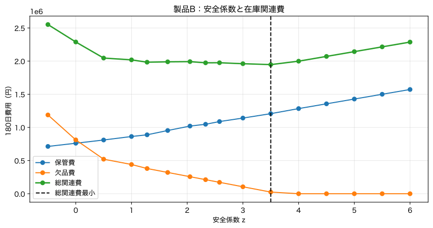
総関連費最小の安全係数: z=3.50 / ¥1,947,283

結果の読み取り

安全係数が低いと欠品費、高いと保管費が増えます。総関連費の谷が経済的な候補ですが、重要顧客や安全部品は費用最小より高いサービス水準を選ぶ場合があります。

欠品費の設定は結論に強く効きます。金額根拠と不確実性を示し、複数シナリオで方針の頑健性を確認します。

No.045：発注ロットサイズをモデル化する

実務での意味

大ロットは発注・段取り回数を減らしますが平均在庫を増やします。EOQは、発注費と保管費の合計が小さくなる基本ロットを示します。

分析・モデル化の考え方

年間需要 $D$ 、1回当たり発注費 $K$ 、1個年間保管費 $h$ のとき、

Q^*=\sqrt{\frac{2DK}{h}}

です。欠品、数量割引、能力、最小ロットは含まないため、初期候補として使います。

Pythonで確認する

eoq_rows = []
for product, group in demand.groupby("product"):
    spec = products.set_index("product").loc[product]
    annual_demand = group["demand_units"].mean() * 365
    annual_holding = spec["holding_cost_day"] * 365
    eoq = np.sqrt(2 * annual_demand * spec["order_cost"] / annual_holding)
    eoq_rows.append({"製品": product, "年間需要": annual_demand, "EOQ": eoq, "現行ロット": spec["current_order_qty"]})
eoq_table = pd.DataFrame(eoq_rows)
display(eoq_table.style.format({"年間需要": "{:,.0f}", "EOQ": "{:,.0f}", "現行ロット": "{:,.0f}"}))

spec_a = products.set_index("product").loc["A"]
annual_demand_a = demand.query("product == 'A'")["demand_units"].mean() * 365
lot_grid = np.arange(300, 2_501, 100)
ordering_cost = annual_demand_a / lot_grid * spec_a["order_cost"]
holding_cost = lot_grid / 2 * spec_a["holding_cost_day"] * 365
fig, ax = plt.subplots()
ax.plot(lot_grid, ordering_cost, label="年間発注費")
ax.plot(lot_grid, holding_cost, label="年間保管費")
ax.plot(lot_grid, ordering_cost + holding_cost, linewidth=2, label="合計")
ax.set_title("製品A：発注ロットと年間関連費")
ax.set_xlabel("発注ロット（個/回）")
ax.set_ylabel("年間費用（円）")
ax.grid(True, alpha=0.3)
ax.legend()
plt.tight_layout()
plt.show()

	製品	年間需要	EOQ	現行ロット
0	A	34,979	1,384	1,400
1	B	23,563	1,024	1,000
2	C	13,286	697	700

$svg$

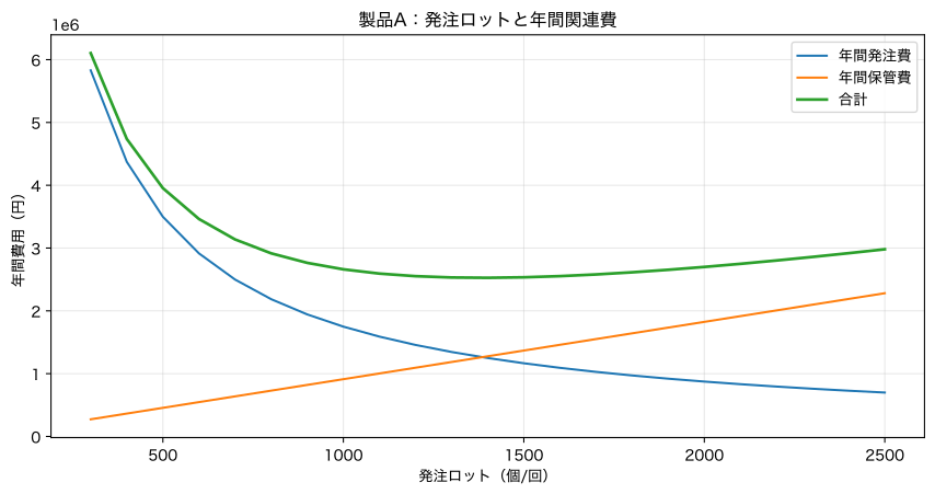
結果の読み取り

ロットを小さくすると発注費、大きくすると保管費が増えます。合計曲線の底付近は比較的平らなため、EOQぴったりではなく荷姿や生産単位へ丸めても影響が小さい場合があります。

実務では最小発注量、パレット数、賞味期限、設備ロット、共同発注を加えます。

No.046：生産能力制約をモデル化する

実務での意味

製品別計画を合計したとき、共通ラインの加工時間と段取り時間を超えれば実行できません。需要増シナリオを能力へ変換します。

分析・モデル化の考え方

\sum_p t_px_p+\sum_p s_py_p\leq H

$t_p$ は1個当たり加工分、 $x_p$ は数量、 $s_p$ は段取り時間、 $y_p$ は生産有無です。週5日・1日22時間の総枠から各製品1回の段取りを引きます。

Pythonで確認する

weekly_demand = demand.groupby("product")["demand_units"].mean() * 7
capacity_rows = []
gross_minutes = 22 * 60 * 5
setup_minutes = products["setup_hours"].sum() * 60
net_minutes = gross_minutes - setup_minutes
for factor, name in [(1.0, "基準"), (1.2, "需要+20%")]:
    required = sum(
        weekly_demand[p] * factor * products.set_index("product").loc[p, "cycle_minutes"]
        for p in weekly_demand.index
    )
    capacity_rows.append({"シナリオ": name, "必要加工時間_分": required, "正味能力_分": net_minutes, "負荷率": required / net_minutes, "余力_分": net_minutes - required})
capacity = pd.DataFrame(capacity_rows)
display(capacity.style.format({"必要加工時間_分": "{:,.0f}", "正味能力_分": "{:,.0f}", "負荷率": "{:.1%}", "余力_分": "{:+,.0f}"}))

fig, ax = plt.subplots()
ax.bar(capacity["シナリオ"], capacity["負荷率"] * 100, color=["#74c476", "#de2d26"])
ax.axhline(100, color="black", linestyle="--", label="能力上限")
ax.set_title("需要シナリオ別の共通ライン負荷率")
ax.set_xlabel("需要シナリオ")
ax.set_ylabel("設備負荷率（%）")
ax.grid(True, axis="y", alpha=0.3)
ax.legend()
plt.tight_layout()
plt.show()

	シナリオ	必要加工時間_分	正味能力_分	負荷率	余力_分
0	基準	5,830	5,880	99.1%	+50
1	需要+20%	6,996	5,880	119.0%	-1,116

$svg$

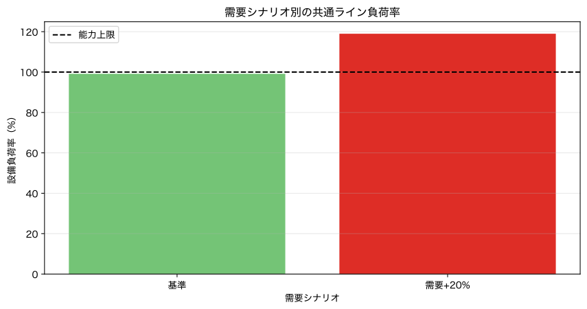
結果の読み取り

基準需要が能力内でも、20%増では上限を超える可能性があります。需要施策や安全在庫積み増しを決める前に、残業、段取り短縮、外注、前倒し生産を検討します。

平均週だけでなくピーク週、保全停止、故障、歩留まり低下もシナリオに含めます。

No.047：段取り替えコストをモデル化する

実務での意味

小ロット化は在庫を減らしますが、段取り回数・停止時間・初品検査・廃棄を増やします。段取りを金額と能力の両面で評価します。

分析・モデル化の考え方

年間段取り回数を $D/Q$ と近似すると、

C_{\mathrm{setup}}(Q)=\frac{D}{Q}K_s,\qquad H_{\mathrm{setup}}(Q)=\frac{D}{Q}s

となります。ロット $Q$ を大きくすると段取り負荷は減りますが、サイクル在庫 $Q/2$ は増えます。

Pythonで確認する

spec_b = products.set_index("product").loc["B"]
annual_demand_b = demand.query("product == 'B'")["demand_units"].mean() * 365
batch_sizes = np.arange(300, 1_801, 100)
changeovers = annual_demand_b / batch_sizes
setup_costs = changeovers * spec_b["setup_cost"]
setup_hours = changeovers * spec_b["setup_hours"]
cycle_inventory_cost = batch_sizes / 2 * spec_b["holding_cost_day"] * 365
setup_eval = pd.DataFrame({
    "ロット": batch_sizes, "年間段取り回数": changeovers,
    "年間段取り時間": setup_hours, "年間段取り費": setup_costs,
    "年間サイクル在庫費": cycle_inventory_cost,
})
setup_eval["合計費用"] = setup_eval["年間段取り費"] + setup_eval["年間サイクル在庫費"]
best_batch = setup_eval.loc[setup_eval["合計費用"].idxmin()]

fig, ax = plt.subplots()
ax.plot(batch_sizes, setup_costs, label="段取り費")
ax.plot(batch_sizes, cycle_inventory_cost, label="サイクル在庫費")
ax.plot(batch_sizes, setup_eval["合計費用"], linewidth=2, label="合計")
ax.axvline(best_batch["ロット"], color="black", linestyle="--", label="合計最小")
ax.set_title("製品B：ロットと段取り・在庫費")
ax.set_xlabel("生産ロット（個/回）")
ax.set_ylabel("年間費用（円）")
ax.grid(True, alpha=0.3)
ax.legend()
plt.tight_layout()
plt.show()
print(f"段取り費と在庫費の合計最小ロット: {best_batch['ロット']:.0f}個")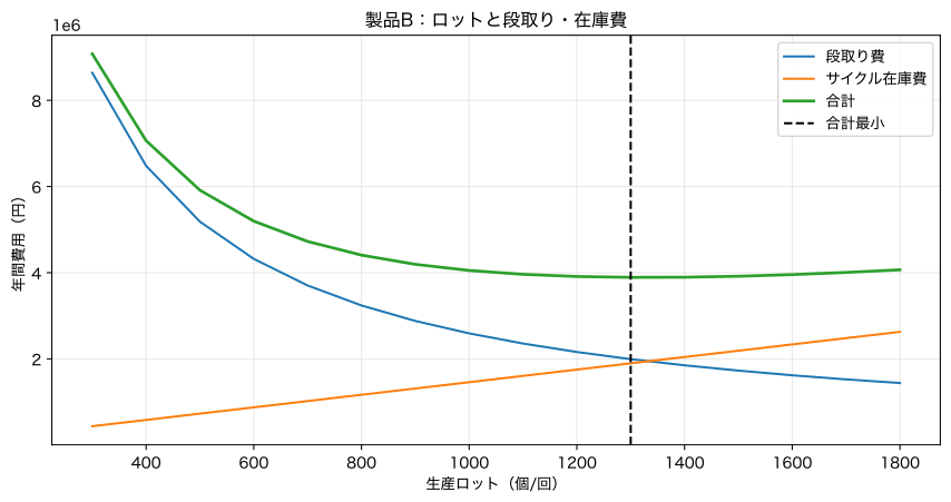

$svg$

段取り費と在庫費の合計最小ロット: 1300個

結果の読み取り

ロットを小さくすると段取り費、大きくすると在庫費が増えます。段取り改善で時間と費用を下げれば、より小ロットで在庫を抑えられます。

段取り費には停止時間だけでなく、洗浄、治具、初品検査、条件安定までの不良を含めます。

No.048：リードタイムをモデル化する

実務での意味

リードタイム短縮は、発注点と安全在庫の両方を下げます。納期短縮施策を在庫金額と欠品耐性へ換算できます。

分析・モデル化の考え方

発注点は $R=\mu L+z\sigma_{DL}$ なので、 $L$ が短くなると平均リードタイム需要と変動バッファが減ります。製品Cについて12日、9日、6日を比較します。

Pythonで確認する

group_c = demand.query("product == 'C'")
spec_c = products.set_index("product").loc["C"]
mu_c, sigma_c = group_c["demand_units"].mean(), group_c["demand_units"].std(ddof=1)
lead_rows = []
for lead in [12, 9, 6]:
    sigma_lt = np.sqrt(lead * sigma_c**2 + mu_c**2 * 1.2**2)
    safety = norm.ppf(0.95) * sigma_lt
    rop = mu_c * lead + safety
    lead_rows.append({"リードタイム_日": lead, "LT平均需要": mu_c * lead, "安全在庫": safety, "発注点": rop, "発注点在庫金額": rop * spec_c["unit_cost"]})
lead_table = pd.DataFrame(lead_rows)
display(lead_table.style.format({
    "LT平均需要": "{:,.0f}", "安全在庫": "{:,.0f}", "発注点": "{:,.0f}", "発注点在庫金額": "¥{:,.0f}"
}))

fig, ax = plt.subplots()
ax.bar(lead_table["リードタイム_日"].astype(str), lead_table["発注点"], color="#9ecae1")
ax.set_title("製品C：リードタイム短縮と発注点")
ax.set_xlabel("リードタイム（日）")
ax.set_ylabel("発注点（個）")
ax.grid(True, axis="y", alpha=0.3)
plt.tight_layout()
plt.show()

	リードタイム_日	LT平均需要	安全在庫	発注点	発注点在庫金額
0	12	437	104	541	¥4,330,150
1	9	328	97	425	¥3,399,549
2	6	218	90	308	¥2,464,433

$svg$

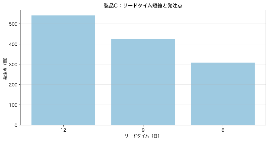
結果の読み取り

リードタイム短縮により、平均需要分と安全在庫の両方が下がり、在庫資金を解放できます。単価の高い製品ほど金額効果が大きくなります。

平均納期だけでなく納期ばらつきを減らすことも重要です。短縮費用と在庫・欠品削減効果を比較します。

No.049：多品種生産計画をモデル化する

実務での意味

共通ラインの能力と材料が不足すると、全需要を同時に満たせません。契約上の最低供給を守りつつ、限界利益が大きい組み合わせを選びます。

分析・モデル化の考え方

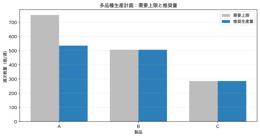
製品別週次生産量 $x_p$ を意思決定変数とし、

\max\sum_pm_px_p

を、加工時間、材料、最低供給、需要上限の制約下で解きます。段取り時間を除いた正味能力は5,880分、材料上限は2,300kgとします。

Pythonで確認する

spec = products.set_index("product")
product_order = ["A", "B", "C"]
weekly_upper = (demand.groupby("product")["demand_units"].mean() * 7 * 1.12).reindex(product_order)
minimum_supply = pd.Series({"A": 500, "B": 340, "C": 190})

c = -spec.loc[product_order, "margin"].to_numpy()
A_ub = np.vstack([
    spec.loc[product_order, "cycle_minutes"].to_numpy(),
    spec.loc[product_order, "material_kg"].to_numpy(),
])
b_ub = np.array([5_880, 2_300])
bounds = [(minimum_supply[p], weekly_upper[p]) for p in product_order]
result = linprog(c, A_ub=A_ub, b_ub=b_ub, bounds=bounds, method="highs")

plan = pd.DataFrame({
    "製品": product_order, "最低供給": minimum_supply.reindex(product_order).to_numpy(),
    "需要上限": weekly_upper.to_numpy(), "推奨生産量": result.x,
    "限界利益_円個": spec.loc[product_order, "margin"].to_numpy(),
})
display(plan.style.format({"最低供給": "{:,.0f}", "需要上限": "{:,.0f}", "推奨生産量": "{:,.0f}", "限界利益_円個": "¥{:,.0f}"}))
used_minutes = A_ub[0] @ result.x
used_material = A_ub[1] @ result.x
print(f"設備時間: {used_minutes:,.0f} / 5,880分、材料: {used_material:,.0f} / 2,300kg")
print(f"週次限界利益: ¥{-result.fun:,.0f}")

fig, ax = plt.subplots()
x_pos = np.arange(len(plan))
ax.bar(x_pos - 0.18, plan["需要上限"], width=0.36, label="需要上限", color="#bdbdbd")
ax.bar(x_pos + 0.18, plan["推奨生産量"], width=0.36, label="推奨生産量", color="#2c7fb8")
ax.set_xticks(x_pos, plan["製品"])
ax.set_title("多品種生産計画：需要上限と推奨量")
ax.set_xlabel("製品")
ax.set_ylabel("週次数量（個/週）")
ax.grid(True, axis="y", alpha=0.3)
ax.legend()
plt.tight_layout()
plt.show()

	製品	最低供給	需要上限	推奨生産量	限界利益_円個
0	A	500	751	535	¥1,400
1	B	340	506	506	¥2,200
2	C	190	285	285	¥3,400

設備時間: 5,880 / 5,880分、材料: 2,295 / 2,300kg
週次限界利益: ¥2,832,662

$svg$

結果の読み取り

制約が効くと、すべての需要上限を満たせず、最低供給と限界利益を考慮した配分になります。未充足分には前倒し在庫、外注、残業、納期調整を検討します。

限界利益だけでなく、重要顧客、契約、欠品費、将来LTVを目的関数や最低供給制約へ反映します。

No.050：在庫・生産モデルの評価指標を整理する

実務での意味

平均在庫だけを最小化すると欠品が増え、充足率だけを最大化すると在庫が膨らみます。複数KPIで方針を比較し、目的に合うバランスを選びます。

分析・モデル化の考え方

評価候補は需要充足率、欠品数、欠品日、平均在庫、保管費、欠品費、発注費、総関連費、発注回数です。ここでは安全係数0.5、1.28、2.05の3方針を全製品で比較します。

Pythonで確認する

policy_names = {0.5: "現行相当", 1.28: "バランス", 2.05: "高サービス"}
policy_rows = []
for z, name in policy_names.items():
    results = [simulate_product(product, z) for product in ["A", "B", "C"]]
    total_demand = demand["demand_units"].sum()
    lost = sum(r["欠品数"] for r in results)
    policy_rows.append({
        "方針": name, "安全係数": z, "需要充足率": 1 - lost / total_demand,
        "欠品数": lost, "平均在庫合計": sum(r["平均在庫"] for r in results),
        "総関連費": sum(r["総関連費"] for r in results),
        "発注回数": sum(r["発注回数"] for r in results),
    })
policy_eval = pd.DataFrame(policy_rows)
display(policy_eval.style.format({
    "需要充足率": "{:.2%}", "欠品数": "{:,.0f}", "平均在庫合計": "{:,.0f}",
    "総関連費": "¥{:,.0f}", "発注回数": "{:,}"
}))

fig, axes = plt.subplots(1, 2, figsize=(11, 4.2))
axes[0].scatter(policy_eval["平均在庫合計"], policy_eval["需要充足率"] * 100, s=90, color="#2c7fb8")
for row in policy_eval.itertuples():
    axes[0].annotate(row.方針, (row.平均在庫合計, row.需要充足率 * 100), xytext=(5, 5), textcoords="offset points")
axes[0].set_title("平均在庫と需要充足率")
axes[0].set_xlabel("平均在庫合計（個）")
axes[0].set_ylabel("需要充足率（%）")
axes[0].grid(True, alpha=0.3)
axes[1].bar(policy_eval["方針"], policy_eval["総関連費"] / 1_000_000, color="#74c476")
axes[1].set_title("方針別の総関連費")
axes[1].set_xlabel("在庫方針")
axes[1].set_ylabel("総関連費（百万円/180日）")
axes[1].grid(True, axis="y", alpha=0.3)
plt.tight_layout()
plt.show()
best_policy = policy_eval.loc[policy_eval["総関連費"].idxmin()]
print(f"総関連費最小: {best_policy['方針']} / 充足率 {best_policy['需要充足率']:.2%} / ¥{best_policy['総関連費']:,.0f}")

	方針	安全係数	需要充足率	欠品数	平均在庫合計	総関連費	発注回数
0	現行相当	0.500000	97.27%	966	1,776	¥5,813,116	31
1	バランス	1.280000	98.38%	573	1,958	¥5,558,008	32
2	高サービス	2.050000	99.03%	344	2,171	¥5,506,581	32

$svg$

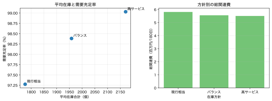
総関連費最小: 高サービス / 充足率 99.03% / ¥5,506,581

結果の読み取り

安全係数を上げると充足率と平均在庫がともに増えます。総関連費最小方針は経済性の候補ですが、顧客要求を満たす最低充足率を先に制約として置く場合もあります。

本番では品目別KPIに加え、緊急発注、納期遵守、廃棄、計画変更、残業、設備負荷を評価します。平均値だけでなく最悪週や変動も確認します。

対象ノックを通して見える実務上の示唆

No.041〜050から、在庫・生産方針は一つのKPIで決められないことが分かります。

在庫方程式で入荷・販売・欠品・期末残高を整合させる
発注点はリードタイム需要と安全在庫に分解する
安全在庫は需要・納期変動とサービス水準から設計する
保管費・欠品費・発注費を同じ尺度で比較する
EOQと段取りモデルでロットと在庫のトレードオフを確認する
製品別計画を共通設備・材料制約で合算する
リードタイム短縮を在庫数量・金額へ換算する
多品種計画では最低供給と経済性を同時に扱う
方針は充足率、在庫、費用、安定性の複数KPIで評価する

欠品を在庫だけで解決せず、予測、納期、段取り、能力、外注を含む選択肢を比較することが重要です。

実務導入する場合に必要なこと

1. 在庫状態と引当ルールを定義する

手元、引当済、発注残、受注残、不良保留、仕掛を区別し、在庫ポジションの計算を統一します。

2. 需要とリードタイムの実績分布を作る

平均だけでなく、曜日・季節・顧客・仕入先別のばらつき、遅延、連続欠品を記録します。

3. 費用パラメータを合意する

保管費、資本費、陳腐化、発注費、段取り費、欠品粗利、緊急輸送、顧客影響の範囲を決めます。

4. 共通能力を正しくモデル化する

設備、作業者、治具、材料、保全、歩留まり、最低ロットを制約へ反映します。

5. 履歴データで方針をバックテストする

同じ需要系列で複数方針を再現し、欠品・平均在庫・費用・発注頻度を比較します。

6. 例外対応と更新責任を決める

需要急増、供給停止、重要顧客、終売品の手動判断を定義し、発注点・費用・能力の更新担当と頻度を決めます。

まとめ

No.041〜050では、多品種交換部品の架空データを使い、在庫・生産モデルの基本を確認しました。

在庫残高を状態方程式で表す
発注点・安全在庫・ロットを需要とリードタイムから設計する
欠品費、保管費、発注費、段取り費を比較する
設備・材料制約下で多品種生産量を決める
充足率、在庫、費用を含む複数KPIで方針を評価する

在庫モデルの価値は、在庫数量を出すことではなく、欠品リスクと資金・能力のトレードオフを関係部署が同じ前提で判断できることにあります。

法人向けのご相談

数理工房では、製造業における次のようなテーマを支援しています。

発注点・安全在庫・発注ロットの設計
欠品費・在庫費を考慮した方針シミュレーション
段取り・設備能力を含む多品種生産計画
リードタイム短縮・外注・残業のシナリオ比較
在庫・生産KPIのダッシュボードと運用設計
生産管理・調達・DX部門向けの実データ型研修

「在庫を減らしたいが欠品が不安」「製品別計画はあるが共通能力に収まらない」という段階から、データ定義、PoC、運用設計までご相談いただけます。

📩 お問い合わせ: surikobo.co.jp/contact まずはお気軽にご相談ください。

欠品・在庫・段取り・能力を同時に考える：多品種交換部品で学ぶ在庫・生産のモデル化

欠品・在庫・段取り・能力を同時に考える

多品種交換部品で学ぶ在庫・生産のモデル化 No.041〜No.050

はじめに：この記事で扱う製造業の実務課題

現場でよくある状況

なぜこの問題は判断が難しいのか

今回扱うノックの全体像

Python 環境の準備

架空データの作成

No.041：在庫残高の変化を数式で表現する

実務での意味

分析・モデル化の考え方

Pythonで確認する

結果の読み取り

No.042：発注点をモデル化する

実務での意味

分析・モデル化の考え方

Pythonで確認する

結果の読み取り

No.043：安全在庫をモデル化する

実務での意味

分析・モデル化の考え方

Pythonで確認する

結果の読み取り

No.044：欠品コストと保管コストをモデル化する

実務での意味

分析・モデル化の考え方

Pythonで確認する

結果の読み取り

No.045：発注ロットサイズをモデル化する

実務での意味

分析・モデル化の考え方

Pythonで確認する

結果の読み取り

No.046：生産能力制約をモデル化する

実務での意味

分析・モデル化の考え方

Pythonで確認する

結果の読み取り

No.047：段取り替えコストをモデル化する

実務での意味

分析・モデル化の考え方

Pythonで確認する

結果の読み取り

No.048：リードタイムをモデル化する

実務での意味

分析・モデル化の考え方

Pythonで確認する

結果の読み取り

No.049：多品種生産計画をモデル化する

実務での意味

分析・モデル化の考え方

Pythonで確認する

結果の読み取り

No.050：在庫・生産モデルの評価指標を整理する

実務での意味

分析・モデル化の考え方

Pythonで確認する

結果の読み取り

対象ノックを通して見える実務上の示唆

実務導入する場合に必要なこと

1. 在庫状態と引当ルールを定義する

2. 需要とリードタイムの実績分布を作る

3. 費用パラメータを合意する

4. 共通能力を正しくモデル化する

5. 履歴データで方針をバックテストする

6. 例外対応と更新責任を決める

まとめ

法人向けのご相談

Related Posts

需要増に備える工場施策を「利益・納期・リスク」で選ぶ

限られた設備・人員・予算を最も価値ある仕事へ配分する

設備・顧客・在庫の「次の状態」を予測する

需要変動と設備故障を「確率」で意思決定へ変える

検査待ちの滞留を人員配置の判断へ変える：工場の最終検査工程で学ぶ待ち行列・混雑のモデル化