100 Exercises / Mathematical modeling / Mathematical Modeling 100 Exercises

Considering stockouts, inventory, planning, and capacity simultaneously: Learning Inventory and Production Modeling through Multi-Variety Replacement Parts

2020-02-07

Considering stockouts, inventory, planning, and capabilities simultaneously

Learning Inventory and Production Modeling with Multi-Variety Replacement Parts No.041–No.050

This article uses three fictional industrial equipment replacement parts as the subject, and continuously models inventory balances, order points, safety stock, shortage costs, storage costs, order lots, production capacity, planning, lead time, and multi-product production plans.

The goal is not simply to reduce inventory or to completely eliminate stockouts. Numerically compare trade-offs between customer service, working capital, setup load, and equipment capacity to select feasible policies..

[!NOTE] This material is a notebook previously used by Surikoubo (or personally by the representative, Kazuyama), and has been reconstructed, edited, and published with the company’s permission. All data listed is fictional and has no relation whatsoever to real companies, factories, or figures.

Introduction: Practical Challenges in Manufacturing Covered in This Article

In a fictional parts factory, replacement parts A, B, and C are produced on a common line. A has a high demand volume, while C has a low demand but has a significant impact on customers when out of stock. Procurement and production lead times vary by product and are sometimes delayed.

While production management wants to increase inventory to avoid stockouts, accounting aims to keep inventory levels low. Smaller-batch production reduces average inventory but increases setup frequency and downtime. When demand increases, it is also necessary to check the constraints of equipment time and materials.

This time, we use 180 days’ worth of hypothetical demand to gradually organize everything from inventory equations to multi-product production planning and model evaluation.

Common situations on site

The relationship between the initial inventory and incoming and shipping items does not match, making it impossible to trace the causes of inventory discrepancies.
The ordering point is based on the manager’s experience value, not reflecting demand fluctuations or lead times.
Safety stock is uniformly set for ○ days, and the impact of shortages is not distinguished by product
Tracking only inventory reduction amounts without aggregating out-of-stock losses or emergency response costs
Smaller batches reduced inventory, but increased planning led to a shortage of capacity.
Even if a product-specific plan is established, when you add up common equipment and materials, the constraints are exceeded.
Policy evaluations are based solely on average inventory and do not compare fulfillment rates, costs, or stability.

Inventory and production are not separate issues. Order volume, scheduling, capacity, and lead times all interact with each other through inventory status.

Why is this issue so difficult to judge?

Increasing inventory can reduce shortages, but it also raises storage costs, financial constraints, and stalemate. Increasing the lot size reduces the number of orders and setups, but increases the average inventory. There is a cap on equipment operating time, and capacity must be allocated to multiple products of varying importance.

Furthermore, demand and lead times are not fixed. If you create ordering points based solely on average demand, you won’t be able to absorb sudden increases in demand or delays in delivery. Therefore, it combines state equations, probabilistic safety stock, cost functions, capability constraints, and evaluation KPIs.

Overview of Exercise covered this time

No.	Theme	Practical Judgment
041	inventory balance	How inventory changes with arrivals, demand, and stockouts
042	Order point	When to start restocking
043	Safety stock	How many to absorb from demand and delivery date fluctuations
044	Shortage and storage fees	How far to raise service standards
045	Order lot	How many to restock at once
046	Production capacity constraints	Whether the demand plan fits within the equipment timeframe
047	Setup change	How to evaluate the cost of small-lot production
048	lead time	How Shorter Delivery Times Affect Inventory
049	Multi-Variety Production Plan	Which products to allocate limited capacity to
050	Evaluation Indicators	How to comprehensively compare costs, inventory, and stockouts

No.041 to 050 follow the process of recording conditions, designing individual product policies, allocating common resources, and conducting comprehensive evaluations.

Preparing the Python environment

No external data is used. Fix random number seeds in NumPy, then use SciPy’s normal distribution, linear programming, pandas, and matplotlib.

%matplotlib inline
%config InlineBackend.figure_format = 'svg'

import platform
import sys

import matplotlib
import matplotlib.pyplot as plt
from matplotlib import font_manager
import numpy as np
import pandas as pd
import scipy
from scipy.optimize import linprog
from scipy.stats import norm
from IPython.display import display

SEED = 42
rng = np.random.default_rng(SEED)
available_fonts = {font.name for font in font_manager.fontManager.ttflist}
plot_font = next((f for f in ["Hiragino Sans", "Yu Gothic", "Noto Sans CJK JP"] if f in available_fonts), "sans-serif")
plt.rcParams["font.family"] = plot_font
plt.rcParams["axes.unicode_minus"] = False
plt.rcParams["figure.figsize"] = (9, 4.8)

print(f"Python     : {sys.version.split()[0]}")
print(f"NumPy      : {np.__version__}")
print(f"pandas     : {pd.__version__}")
print(f"SciPy      : {scipy.__version__}")
print(f"matplotlib : {matplotlib.__version__}")
print(f"plot font  : {plot_font}")
print(f"platform   : {platform.platform()}")
print(f"random seed: {SEED}")

Python     : 3.13.1
NumPy      : 2.5.1
pandas     : 3.0.3
SciPy      : 1.18.0
matplotlib : 3.11.0
plot font  : Hiragino Sans
platform   : macOS-26.3-arm64-arm-64bit-Mach-O
random seed: 42

Creation of Fictional Data

Generate daily demand for 180 days for products A, B, and C. Average demand, standard lead time, storage costs, shortage costs, order costs, unit prices, processing time, and setup time vary for each product.

The current policy is to order points and fixed lots with a safety factor of $z=0.5$ . One replenishment every five causes a 3-day delay, reproducing shortages caused by sudden demand surges and delivery schedule fluctuations.

dates = pd.date_range("2025-01-01", periods=180, freq="D")
products = pd.DataFrame({
    "product": ["A", "B", "C"],
    "base_daily_demand": [110, 74, 42],
    "standard_lead_days": [5, 8, 12],
    "holding_cost_day": [5, 8, 12],
    "shortage_cost_unit": [1_000, 1_600, 2_500],
    "order_cost": [50_000, 65_000, 80_000],
    "unit_cost": [3_500, 5_200, 8_000],
    "current_order_qty": [1_400, 1_000, 700],
    "cycle_minutes": [3.0, 4.5, 7.0],
    "setup_hours": [3.0, 4.0, 5.0],
    "setup_cost": [80_000, 110_000, 150_000],
    "margin": [1_400, 2_200, 3_400],
    "material_kg": [1.2, 1.8, 2.6],
})

demand_rows = []
for day_no, date in enumerate(dates):
    weekday_factor = 0.48 if date.dayofweek >= 5 else 1.0
    seasonal = 1 + 0.12 * np.sin(2 * np.pi * (day_no - 35) / 180)
    spike = 1.45 if rng.random() < 0.045 else 1.0
    for spec in products.itertuples(index=False):
        expected = spec.base_daily_demand * weekday_factor * seasonal * spike
        demand_rows.append({
            "date": date,
            "day_no": day_no,
            "product": spec.product,
            "expected_demand": expected,
            "demand_units": rng.poisson(max(1, expected)),
        })

demand = pd.DataFrame(demand_rows).merge(products, on="product", how="left")

history = []
for product, group in demand.groupby("product", sort=False):
    group = group.sort_values("date").reset_index(drop=True)
    spec = products.set_index("product").loc[product]
    mu, sigma = group["demand_units"].mean(), group["demand_units"].std(ddof=1)
    reorder_point = int(round(mu * spec["standard_lead_days"] + 0.5 * sigma * np.sqrt(spec["standard_lead_days"])))
    order_qty = int(spec["current_order_qty"])
    arrivals = np.zeros(len(group) + 30, dtype=int)
    on_hand = reorder_point + order_qty
    order_count = 0
    for i, row in group.iterrows():
        arrival = int(arrivals[i])
        begin = on_hand
        on_hand += arrival
        sales = min(on_hand, int(row["demand_units"]))
        shortage = int(row["demand_units"]) - sales
        on_hand -= sales
        inventory_position = on_hand + int(arrivals[i + 1:].sum())
        placed = 0
        if inventory_position <= reorder_point:
            placed = order_qty
            order_count += 1
            delay = 3 if order_count % 5 == 0 else 0
            arrivals[i + int(spec["standard_lead_days"]) + delay] += placed
        history.append({
            **row.to_dict(), "begin_inventory": begin, "arrival_units": arrival,
            "sales_units": sales, "shortage_units": shortage,
            "ending_inventory": on_hand, "order_units": placed,
            "current_reorder_point": reorder_point,
        })

inventory_data = pd.DataFrame(history)
print(f"Number of records: {len(inventory_data):,}Walk (180days × 3Products)")
display(inventory_data.head(9).style.format({"expected_demand": "{:.1f}"}))

Number of records: 540 lines (180 days, × 3 products)

	date	day_no	product	expected_demand	demand_units	base_daily_demand	standard_lead_days	holding_cost_day	shortage_cost_unit	order_cost	unit_cost	current_order_qty	cycle_minutes	setup_hours	setup_cost	margin	material_kg	begin_inventory	sales_units	ending_inventory	current_reorder_point
0	2025-01-01 00:00:00	0	A	97.6	96	110	5	5	1000	50000	3500	1400	3.000000	3.000000	80000	1400	1.200000	1914	96	1818	514
1	2025-01-02 00:00:00	1	A	97.8	94	110	5	5	1000	50000	3500	1400	3.000000	3.000000	80000	1400	1.200000	1818	94	1724	514
2	2025-01-03 00:00:00	2	A	97.9	79	110	5	5	1000	50000	3500	1400	3.000000	3.000000	80000	1400	1.200000	1724	79	1645	514
3	2025-01-04 00:00:00	3	A	47.1	53	110	5	5	1000	50000	3500	1400	3.000000	3.000000	80000	1400	1.200000	1645	53	1592	514
4	2025-01-05 00:00:00	4	A	47.2	67	110	5	5	1000	50000	3500	1400	3.000000	3.000000	80000	1400	1.200000	1592	67	1525	514
5	2025-01-06 00:00:00	5	A	98.6	90	110	5	5	1000	50000	3500	1400	3.000000	3.000000	80000	1400	1.200000	1525	90	1435	514
6	2025-01-07 00:00:00	6	A	98.8	109	110	5	5	1000	50000	3500	1400	3.000000	3.000000	80000	1400	1.200000	1435	109	1326	514
7	2025-01-08 00:00:00	7	A	143.6	154	110	5	5	1000	50000	3500	1400	3.000000	3.000000	80000	1400	1.200000	1326	154	1172	514
8	2025-01-09 00:00:00	8	A	99.3	85	110	5	5	1000	50000	3500	1400	3.000000	3.000000	80000	1400	1.200000	1172	85	1087	514

overview = inventory_data.groupby("product", as_index=False).agg(
    need=("demand_units", "sum"), sales=("sales_units", "sum"),
    missing_item=("shortage_units", "sum"), average_inventory=("ending_inventory", "mean"),
    out_of_stock_date=("shortage_units", lambda x: (x > 0).sum()),
    number_of_orders=("order_units", lambda x: (x > 0).sum()),
)
overview["required_adequacy_rate"] = overview["sales"] / overview["need"]
display(overview.style.format({"average_inventory": "{:,.1f}", "required_adequacy_rate": "{:.2%}"}))

fig, axes = plt.subplots(1, 2, figsize=(11, 4.2))
for product, group in inventory_data.groupby("product"):
    axes[0].plot(group["date"], group["ending_inventory"], linewidth=1, label=product)
axes[0].set_title("Daily Ending Inventory by Product")
axes[0].set_xlabel("Date")
axes[0].set_ylabel("Ending inventory (units)")
axes[0].grid(True, alpha=0.3)
axes[0].legend(title="Products")
axes[1].bar(overview["product"], overview["required_adequacy_rate"] * 100, color="#2c7fb8")
axes[1].set_title("Current Policy Demand Fulfillment Rate")
axes[1].set_xlabel("Products")
axes[1].set_ylabel("Required sufficiency rate (%）")
axes[1].grid(True, axis="y", alpha=0.3)
plt.tight_layout()
plt.show()
print(f"Total Shortages for All Products: {inventory_data['shortage_units'].sum():,}units")

	product	need	sales	missing_item	average_inventory	out_of_stock_date	number_of_orders	required_adequacy_rate
0	A	17250	16558	692	751.3	7	11	95.99%
1	B	11620	11210	410	550.7	7	11	96.47%
2	C	6552	6354	198	407.6	7	9	96.98%

$svg$

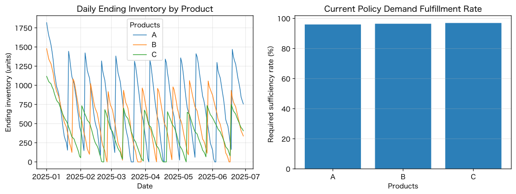
Total missing items for all products: 1,300 units

No.041: Expressing Changes in Inventory Balance with Formulas

Meaning in Practice

Since inventory carries over the previous day’s status, it is necessary to align inventory, sales, and out-of-stock in chronological order. The inventory equation serves as the foundation for checking and simulating book discrepancies.

Approach to Analysis and Modeling

I_t^{\mathrm{end}}=I_t^{\mathrm{begin}}+R_t-S_t

S_t=\min(D_t,I_t^{\mathrm{begin}}+R_t),\qquad U_t=D_t-S_t

$R_t$ is in stock, $S_t$ is for sale, and $U_t$ is out of stock. As a lost order type, out-of-stock items are not carried over to the next day. If the order is backlogged, we add the backorder status.

Check with Python

balance = inventory_data.query("product == 'A'").head(30).copy()
balance["Calculation of ending inventory"] = balance["begin_inventory"] + balance["arrival_units"] - balance["sales_units"]
balance["Inventory discrepancies"] = balance["Calculation of ending inventory"] - balance["ending_inventory"]
display(balance[[
    "date", "begin_inventory", "arrival_units", "demand_units", "sales_units",
    "shortage_units", "ending_inventory", "Inventory discrepancies"
]].style.format({"date": "{:%m-%d}"}))

fig, ax = plt.subplots()
ax.step(balance["date"], balance["ending_inventory"], where="post", label="ending inventory", color="#2c7fb8")
ax.scatter(balance.loc[balance["arrival_units"] > 0, "date"], balance.loc[balance["arrival_units"] > 0, "ending_inventory"], color="#2ca25f", label="Arrival date")
ax.set_title("ProductsA: Inventory trends based on arrivals and demand")
ax.set_xlabel("Date")
ax.set_ylabel("Ending inventory (units)")
ax.grid(True, alpha=0.3)
ax.legend()
plt.xticks(rotation=45)
plt.tight_layout()
plt.show()
print(f"Maximum variance in the inventory equation: {balance['Inventory discrepancies'].abs().max()}units")

	date	begin_inventory	arrival_units	demand_units	sales_units	ending_inventory
0	01-01	1914	0	96	96	1818
1	01-02	1818	0	94	94	1724
2	01-03	1724	0	79	79	1645
3	01-04	1645	0	53	53	1592
4	01-05	1592	0	67	67	1525
5	01-06	1525	0	90	90	1435
6	01-07	1435	0	109	109	1326
7	01-08	1326	0	154	154	1172
8	01-09	1172	0	85	85	1087
9	01-10	1087	0	101	101	986
10	01-11	986	0	43	43	943
11	01-12	943	0	55	55	888
12	01-13	888	0	106	106	782
13	01-14	782	0	117	117	665
14	01-15	665	0	117	117	548
15	01-16	548	0	110	110	438
16	01-17	438	0	99	99	339
17	01-18	339	0	51	51	288
18	01-19	288	0	37	37	251
19	01-20	251	0	98	98	153
20	01-21	153	1400	109	109	1444
21	01-22	1444	0	95	95	1349
22	01-23	1349	0	124	124	1225
23	01-24	1225	0	113	113	1112
24	01-25	1112	0	45	45	1067
25	01-26	1067	0	44	44	1023
26	01-27	1023	0	106	106	917
27	01-28	917	0	93	93	824
28	01-29	824	0	132	132	692
29	01-30	692	0	94	94	598

$svg$

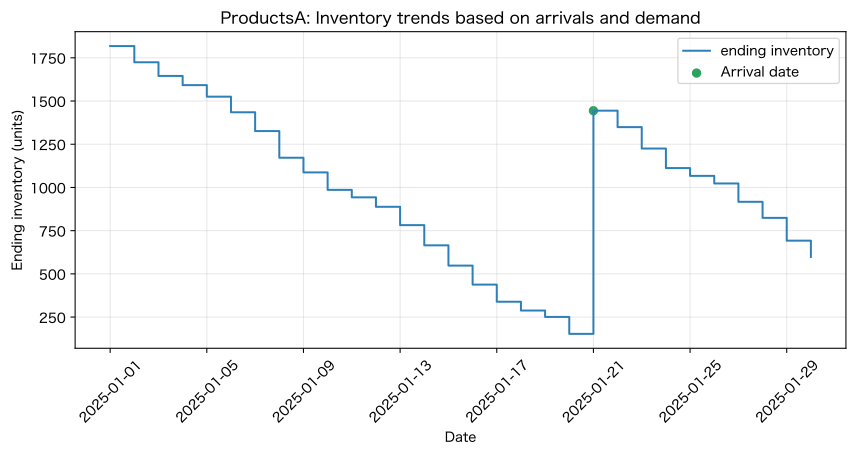
Maximum variance in inventory equations: 0 pieces

Reading the results

You can observe a sawtooth pattern where inventory decreases due to demand and gradually increases on the day of arrival. Since the inventory discrepancy is zero, inbound and outbound inventories and year-end inventory are consistent.

In practice, we distinguish between acceptance points, reserve inventory, defective pending, work-in-progress, and inventory corrections. It is important not to confuse available inventory with accounting stock.

No.042: Modeling Order Points

Meaning in Practice

The order point determines how many inventory positions combining the current inventory and order balance will be replenished. If it’s too late, it will go out of stock; if too early, inventory will increase.

Approach to Analysis and Modeling

R=\mu_D L+SS

$\mu_D L$ is the average demand during lead times, and $SS$ is safety stock. For judgment, use inventory positions that include both order and order backlogs, rather than inventory.

Check with Python

reorder_rows = []
for product, group in inventory_data.groupby("product"):
    spec = products.set_index("product").loc[product]
    mu = group["demand_units"].mean()
    sigma = group["demand_units"].std(ddof=1)
    lead = spec["standard_lead_days"]
    safety_95 = norm.ppf(0.95) * sigma * np.sqrt(lead)
    reorder_rows.append({
        "Products": product, "average_daily_demand": mu, "StandardLT_days": lead,
        "LTaverage_need": mu * lead, "95%Safety stock": safety_95,
        "Recommended Order Points": mu * lead + safety_95,
        "Current Ordering Points": group["current_reorder_point"].iloc[0],
    })
reorder_table = pd.DataFrame(reorder_rows)
display(reorder_table.style.format({
    "average_daily_demand": "{:.1f}", "LTaverage_need": "{:.1f}",
    "95%Safety stock": "{:.1f}", "Recommended Order Points": "{:.0f}", "Current Ordering Points": "{:.0f}"
}))

	Products	average_daily_demand	StandardLT_days	LTaverage_need	95%Safety stock	Recommended Order Points	Current Ordering Points
0	A	95.8	5.000000	479.2	112.9	592	514
1	B	64.6	8.000000	516.4	104.1	621	548
2	C	36.4	12.000000	436.8	75.8	513	460

Reading the results

Currently, the order point has a safety factor of 0.5, while the recommended example has a 95% service level, so the latter is higher. Raising the order point increases delay tolerance, but also increases average inventory.

Order points are reviewed in line with demand forecasts and lead time updates. For highly seasonal products, we use time-based order points rather than fixed values.

No.043: Modeling Safety Stock

Meaning in Practice

Safety stock is a buffer that absorbs orders exceeding average demand and delivery times above average. Adjust target service levels according to product importance.

Approach to Analysis and Modeling

When both demand and lead time fluctuate, the approximate standard deviation

\sigma_{DL}=\sqrt{L\sigma_D^2+\mu_D^2\sigma_L^2}

and the safety stock is $SS=z\sigma_{DL}$ . $z$ is the quantile of the standard normal distribution corresponding to the service level.

Check with Python

service_levels = [0.90, 0.95, 0.99]
rows = []
lead_sigma = 1.2
for product, group in inventory_data.groupby("product"):
    spec = products.set_index("product").loc[product]
    mu, sigma = group["demand_units"].mean(), group["demand_units"].std(ddof=1)
    sigma_lead_demand = np.sqrt(spec["standard_lead_days"] * sigma**2 + mu**2 * lead_sigma**2)
    for level in service_levels:
        z = norm.ppf(level)
        rows.append({"Products": product, "Service level": level, "z": z, "Safety stock": z * sigma_lead_demand})
safety_table = pd.DataFrame(rows)
display(safety_table.pivot(index="Products", columns="Service level", values="Safety stock").style.format("{:.0f}units"))

fig, ax = plt.subplots()
for product, group in safety_table.groupby("Products"):
    ax.plot(group["Service level"] * 100, group["Safety stock"], marker="o", label=product)
ax.set_title("Target Service Levels and Safety Stock")
ax.set_xlabel("Target Service Level (%）")
ax.set_ylabel("Safety stock (units)")
ax.grid(True, alpha=0.3)
ax.legend(title="Products")
plt.tight_layout()
plt.show()

Service level	0.900000	0.950000	0.990000
Products
A	172units	220units	312units
B	128units	165units	233units
C	81units	104units	148units

$svg$

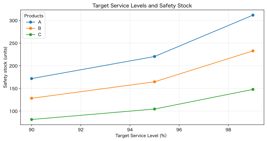
Reading the results

The closer it gets to 99%, the more the required safety stock increases. Products with higher demand volume, demand fluctuations, and lead times require buffers.

Safety stock does not guarantee zero out-of-stock. Distortions in demand distribution, continuous out-of-stock, and supply stoppages are checked in separate scenarios, and parts for critical customers are set at high levels.

No.044: Modeling out-of-stock costs and storage costs

Meaning in Practice

Increasing safety stock raises storage costs and reduces out-of-stock costs. Comparing both on the same cost scale allows you to consider the level of economic service.

Approach to Analysis and Modeling

C(z) = h\sum_t I_t+c_s\sum_t U_t+K\times\text{number of orders}

$h$ is the storage cost per piece per day, $c_s$ is the loss per missing item, and $K$ is the order cost. Shortage fees include lost order gross profit, urgent shipping, and customer impact.

Check with Python

def simulate_product(product, z, order_qty=None, lead_override=None):
    group = demand.query("product == @product").sort_values("date").reset_index(drop=True)
    spec = products.set_index("product").loc[product]
    mu, sigma = group["demand_units"].mean(), group["demand_units"].std(ddof=1)
    lead = int(lead_override or spec["standard_lead_days"])
    sigma_lt = np.sqrt(lead * sigma**2 + mu**2 * 1.2**2)
    rop = mu * lead + z * sigma_lt
    qty = float(order_qty or spec["current_order_qty"])
    arrivals = np.zeros(len(group) + 40)
    on_hand, lost, orders = rop + qty, 0.0, 0
    inv_history = []
    for i, d in enumerate(group["demand_units"].to_numpy()):
        on_hand += arrivals[i]
        sold = min(on_hand, d)
        lost += d - sold
        on_hand -= sold
        position = on_hand + arrivals[i + 1:].sum()
        if position <= rop:
            orders += 1
            delay = 3 if orders % 5 == 0 else 0
            arrivals[i + lead + delay] += qty
        inv_history.append(on_hand)
    holding = np.sum(inv_history) * spec["holding_cost_day"]
    shortage = lost * spec["shortage_cost_unit"]
    ordering = orders * spec["order_cost"]
    return {"z": z, "required_adequacy_rate": 1 - lost / group["demand_units"].sum(), "average_inventory": np.mean(inv_history),
            "number_of_items_out_of_stock": lost, "Storage fee": holding, "Shortage Fee": shortage, "Order cost": ordering,
            "Total Related Expenses": holding + shortage + ordering, "number_of_orders": orders}

cost_comparison = pd.DataFrame([simulate_product("B", z) for z in [-0.5, 0, 0.5, 1.0, 1.28, 1.65, 2.05, 2.33, 2.58, 3.0, 3.5, 4.0, 4.5, 5.0, 5.5, 6.0]])
best_cost = cost_comparison.loc[cost_comparison["Total Related Expenses"].idxmin()]
display(cost_comparison.style.format({
    "required_adequacy_rate": "{:.2%}", "average_inventory": "{:,.0f}", "number_of_items_out_of_stock": "{:,.0f}",
    "Storage fee": "¥{:,.0f}", "Shortage Fee": "¥{:,.0f}", "Order cost": "¥{:,.0f}", "Total Related Expenses": "¥{:,.0f}"
}))

fig, ax = plt.subplots()
ax.plot(cost_comparison["z"], cost_comparison["Storage fee"], marker="o", label="Storage fee")
ax.plot(cost_comparison["z"], cost_comparison["Shortage Fee"], marker="o", label="Shortage Fee")
ax.plot(cost_comparison["z"], cost_comparison["Total Related Expenses"], marker="o", linewidth=2, label="Total Related Expenses")
ax.axvline(best_cost["z"], color="black", linestyle="--", label="Minimum total related costs")
ax.set_title("ProductsB: Safety factor and inventory-related costs")
ax.set_xlabel("safety factor z")
ax.set_ylabel("180Daily cost (yen)")
ax.grid(True, alpha=0.3)
ax.legend()
plt.tight_layout()
plt.show()
print(f"Minimum safety factor for total related expenses: z={best_cost['z']:.2f} / ¥{best_cost['Total Related Expenses']:,.0f}")

	z	required_adequacy_rate	average_inventory	number_of_items_out_of_stock	Storage fee	Shortage Fee	Order cost	Total Related Expenses	number_of_orders
0	-0.500000	93.61%	495	743	¥713,345	¥1,188,115	¥650,000	¥2,551,460	10
1	0.000000	95.63%	529	508	¥761,452	¥812,089	¥715,000	¥2,288,540	11
2	0.500000	97.20%	563	326	¥810,259	¥520,863	¥715,000	¥2,046,122	11
3	1.000000	97.63%	599	276	¥863,093	¥440,837	¥715,000	¥2,018,930	11
4	1.280000	97.96%	617	238	¥888,614	¥380,023	¥715,000	¥1,983,637	11
5	1.650000	98.27%	662	201	¥953,487	¥320,804	¥715,000	¥1,989,290	11
6	2.050000	98.62%	709	160	¥1,020,387	¥256,783	¥715,000	¥1,992,170	11
7	2.330000	98.86%	727	132	¥1,047,433	¥211,968	¥715,000	¥1,974,402	11
8	2.580000	99.08%	756	107	¥1,088,439	¥171,955	¥715,000	¥1,975,394	11
9	3.000000	99.44%	792	65	¥1,141,165	¥104,734	¥715,000	¥1,960,898	11
10	3.500000	99.87%	839	15	¥1,207,576	¥24,708	¥715,000	¥1,947,283	11
11	4.000000	100.00%	892	0	¥1,283,986	¥0	¥715,000	¥1,998,986	11
12	4.500000	100.00%	942	0	¥1,356,010	¥0	¥715,000	¥2,071,010	11
13	5.000000	100.00%	992	0	¥1,428,033	¥0	¥715,000	¥2,143,033	11
14	5.500000	100.00%	1,042	0	¥1,500,056	¥0	¥715,000	¥2,215,056	11
15	6.000000	100.00%	1,092	0	¥1,572,079	¥0	¥715,000	¥2,287,079	11

$svg$

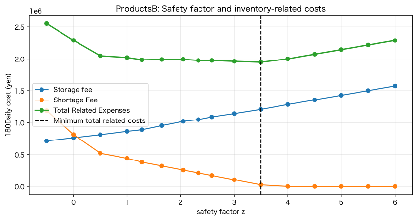
Minimum safety factor for total related costs: z = 3.50 / ¥1,947,283

Reading the results

A low safety factor leads to shortage costs, while a high safety factor increases storage costs. The valley of total related expenses is an economic candidate, but important customers and safety parts may choose service levels higher than the minimum cost.

Setting a shortage fee strongly influences the conclusion. Demonstrate the basis for the amount and uncertainty, and confirm the robustness of policies across multiple scenarios.

No.045: Modeling Order Lot Sizes

Meaning in Practice

Large lots reduce the number of orders and setup cycles but increase average inventory. EOQ indicates the base lot where the sum of order and storage costs decreases.

Approach to Analysis and Modeling

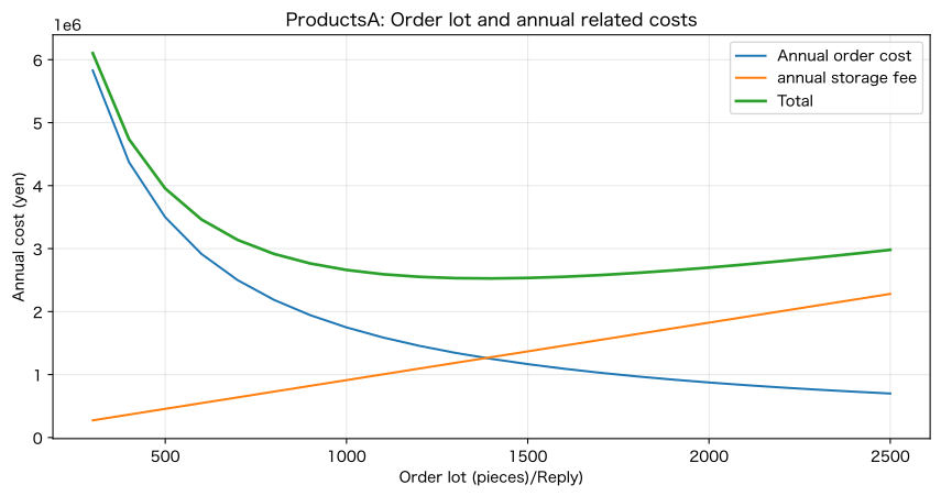
If the annual demand is $D$ , the order cost per shipment is $K$ , and the storage cost per unit is $h$ ,

Q^*=\sqrt{\frac{2DK}{h}}

That’s right. Since out-of-stock, quantity discounts, capacity, and minimum lot are not included, they are used as initial candidates.

Check with Python

eoq_rows = []
for product, group in demand.groupby("product"):
    spec = products.set_index("product").loc[product]
    annual_demand = group["demand_units"].mean() * 365
    annual_holding = spec["holding_cost_day"] * 365
    eoq = np.sqrt(2 * annual_demand * spec["order_cost"] / annual_holding)
    eoq_rows.append({"Products": product, "annual demand": annual_demand, "EOQ": eoq, "Current Lot": spec["current_order_qty"]})
eoq_table = pd.DataFrame(eoq_rows)
display(eoq_table.style.format({"annual demand": "{:,.0f}", "EOQ": "{:,.0f}", "Current Lot": "{:,.0f}"}))

spec_a = products.set_index("product").loc["A"]
annual_demand_a = demand.query("product == 'A'")["demand_units"].mean() * 365
lot_grid = np.arange(300, 2_501, 100)
ordering_cost = annual_demand_a / lot_grid * spec_a["order_cost"]
holding_cost = lot_grid / 2 * spec_a["holding_cost_day"] * 365
fig, ax = plt.subplots()
ax.plot(lot_grid, ordering_cost, label="Annual order cost")
ax.plot(lot_grid, holding_cost, label="annual storage fee")
ax.plot(lot_grid, ordering_cost + holding_cost, linewidth=2, label="Total")
ax.set_title("ProductsA: Order lot and annual related costs")
ax.set_xlabel("Order lot (pieces)/Reply)")
ax.set_ylabel("Annual cost (yen)")
ax.grid(True, alpha=0.3)
ax.legend()
plt.tight_layout()
plt.show()

	Products	annual demand	EOQ	Current Lot
0	A	34,979	1,384	1,400
1	B	23,563	1,024	1,000
2	C	13,286	697	700

$svg$

Reading the results

Smaller lots increase order costs, while larger ones increase storage costs. Since the bottom of the total curve is relatively flat, the EOQ may not be exactly right, and rounding it into the package shape or production unit may have little impact.

In practice, the minimum order quantity, number of pallets, expiration date, equipment lots, and joint orders are added.

No.046: Modeling Production Capacity Constraints

Meaning in Practice

When summing product-specific plans, if the processing and setup times for common lines are exceeded, execution cannot be carried out. Convert demand increase scenarios into capabilities.

Approach to Analysis and Modeling

\sum_p t_px_p+\sum_p s_py_p\leq H

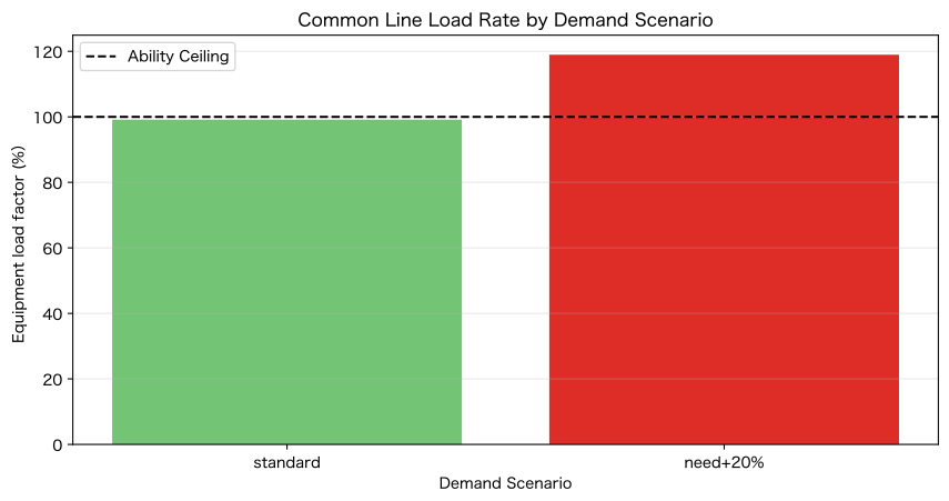
$t_p$ is the amount processed per piece, $x_p$ is the quantity, $s_p$ is setup time, and $y_p$ is whether production is available. From the total slot of 5 days a week and 22 hours per day, one preparation for each product is subtracted.

Check with Python

weekly_demand = demand.groupby("product")["demand_units"].mean() * 7
capacity_rows = []
gross_minutes = 22 * 60 * 5
setup_minutes = products["setup_hours"].sum() * 60
net_minutes = gross_minutes - setup_minutes
for factor, name in [(1.0, "standard"), (1.2, "need+20%")]:
    required = sum(
        weekly_demand[p] * factor * products.set_index("product").loc[p, "cycle_minutes"]
        for p in weekly_demand.index
    )
    capacity_rows.append({"Scenario": name, "Required processing time_minutes": required, "net capability_minutes": net_minutes, "load factor": required / net_minutes, "surplus strength_minutes": net_minutes - required})
capacity = pd.DataFrame(capacity_rows)
display(capacity.style.format({"Required processing time_minutes": "{:,.0f}", "net capability_minutes": "{:,.0f}", "load factor": "{:.1%}", "surplus strength_minutes": "{:+,.0f}"}))

fig, ax = plt.subplots()
ax.bar(capacity["Scenario"], capacity["load factor"] * 100, color=["#74c476", "#de2d26"])
ax.axhline(100, color="black", linestyle="--", label="Ability Ceiling")
ax.set_title("Common Line Load Rate by Demand Scenario")
ax.set_xlabel("Demand Scenario")
ax.set_ylabel("Equipment load factor (%）")
ax.grid(True, axis="y", alpha=0.3)
ax.legend()
plt.tight_layout()
plt.show()

	Scenario	Required processing time_minutes	net capability_minutes	load factor	surplus strength_minutes
0	standard	5,830	5,880	99.1%	+50
1	need+20%	6,996	5,880	119.0%	-1,116

$svg$

Reading the results

Even if the baseline demand is within capacity, a 20% increase may exceed the upper limit. Before deciding on demand measures or increasing safety stock, we consider overtime, shortened setup times, outsourcing, and accelerated production.

Not only average weeks but also peak weeks, maintenance stoppages, breakdowns, and yield declines are included in the scenario.

No.047: Modeling Setup Costs

Meaning in Practice

Small-lot production reduces inventory but increases the number of setup cycles, downtime, initial product inspection, and disposal. We evaluate the arrangement based on both cost and capability.

Approach to Analysis and Modeling

If the annual number of setup cycles is approximated to $D/Q$ ,

C_{\mathrm{setup}}(Q)=\frac{D}{Q}K_s,\qquad H_{\mathrm{setup}}(Q)=\frac{D}{Q}s

That’s how it works. Increasing the lot $Q$ reduces setup load but increases cycle inventory $Q/2$ .

Check with Python

spec_b = products.set_index("product").loc["B"]
annual_demand_b = demand.query("product == 'B'")["demand_units"].mean() * 365
batch_sizes = np.arange(300, 1_801, 100)
changeovers = annual_demand_b / batch_sizes
setup_costs = changeovers * spec_b["setup_cost"]
setup_hours = changeovers * spec_b["setup_hours"]
cycle_inventory_cost = batch_sizes / 2 * spec_b["holding_cost_day"] * 365
setup_eval = pd.DataFrame({
    "lot": batch_sizes, "Number of Annual Arrangements": changeovers,
    "Annual Setup Time": setup_hours, "Annual Setup Fee": setup_costs,
    "Annual cycle inventory cost": cycle_inventory_cost,
})
setup_eval["Total cost"] = setup_eval["Annual Setup Fee"] + setup_eval["Annual cycle inventory cost"]
best_batch = setup_eval.loc[setup_eval["Total cost"].idxmin()]

fig, ax = plt.subplots()
ax.plot(batch_sizes, setup_costs, label="Setup Costs")
ax.plot(batch_sizes, cycle_inventory_cost, label="Cycle inventory cost")
ax.plot(batch_sizes, setup_eval["Total cost"], linewidth=2, label="Total")
ax.axvline(best_batch["lot"], color="black", linestyle="--", label="Minimum total")
ax.set_title("ProductsB: Lot size, planning, and inventory costs")
ax.set_xlabel("Production lot (pieces)/Reply)")
ax.set_ylabel("Annual cost (yen)")
ax.grid(True, alpha=0.3)
ax.legend()
plt.tight_layout()
plt.show()
print(f"Minimum total lot size for setup and inventory costs: {best_batch['lot']:.0f}units")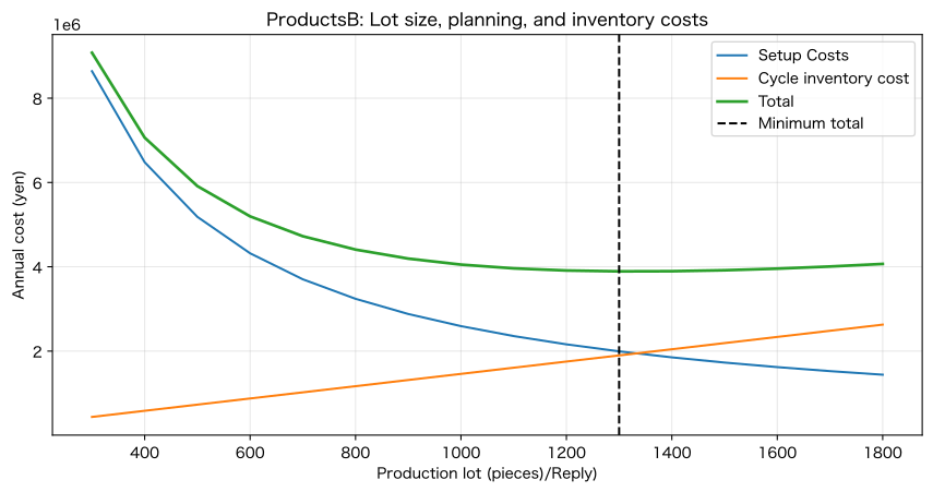

$svg$

Total minimum lot for setup and inventory costs: 1,300 pieces

Reading the results

Reducing the lot size increases setup costs, while increasing the quantity increases inventory costs. By improving the setup to reduce time and costs, you can keep inventory down with smaller lots.

Setup costs include not only downtime but also cleaning, jigs, initial product inspection, and defects until conditions stabilize.

No.048: Modeling Lead Time

Meaning in Practice

Shortening lead times lowers both the order point and safety stock. You can convert delivery shortening measures into inventory value and shortage tolerance.

Approach to Analysis and Modeling

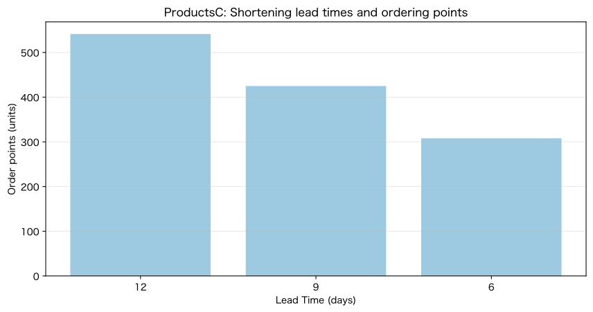
Since the order point is $R=\mu L+z\sigma_{DL}$ , shorter $L$ reduces average lead time demand and variable buffers. Compare 12, 9, and 6 days for Product C.

Check with Python

group_c = demand.query("product == 'C'")
spec_c = products.set_index("product").loc["C"]
mu_c, sigma_c = group_c["demand_units"].mean(), group_c["demand_units"].std(ddof=1)
lead_rows = []
for lead in [12, 9, 6]:
    sigma_lt = np.sqrt(lead * sigma_c**2 + mu_c**2 * 1.2**2)
    safety = norm.ppf(0.95) * sigma_lt
    rop = mu_c * lead + safety
    lead_rows.append({"lead time_days": lead, "LTaverage_need": mu_c * lead, "Safety stock": safety, "Order point": rop, "Order point inventory amount": rop * spec_c["unit_cost"]})
lead_table = pd.DataFrame(lead_rows)
display(lead_table.style.format({
    "LTaverage_need": "{:,.0f}", "Safety stock": "{:,.0f}", "Order point": "{:,.0f}", "Order point inventory amount": "¥{:,.0f}"
}))

fig, ax = plt.subplots()
ax.bar(lead_table["lead time_days"].astype(str), lead_table["Order point"], color="#9ecae1")
ax.set_title("ProductsC: Shortening lead times and ordering points")
ax.set_xlabel("Lead Time (days)")
ax.set_ylabel("Order points (units)")
ax.grid(True, axis="y", alpha=0.3)
plt.tight_layout()
plt.show()

	lead time_days	LTaverage_need	Safety stock	Order point	Order point inventory amount
0	12	437	104	541	¥4,330,150
1	9	328	97	425	¥3,399,549
2	6	218	90	308	¥2,464,433

$svg$

Reading the results

Shorter lead times reduce both average demand and safety stock, freeing up inventory funds. The higher the unit price, the greater the value effect.

It is important not only to have average delivery times but also to reduce delivery variation. Compare cost reduction with the effectiveness of reducing inventory and stockouts.

No.049: Modeling Multi-Variety Production Plans

Meaning in Practice

If the capacity and materials of the common line are insufficient, it will be impossible to meet all demand simultaneously. Choose combinations that maintain the contractual minimum supply while having a large marginal profit.

Approach to Analysis and Modeling

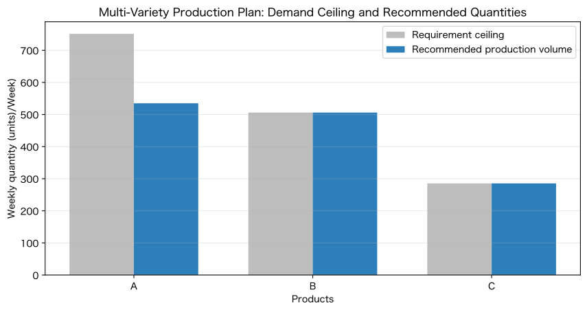
Weekly production volume by product $x_p$ is used as the decision variable,

\max\sum_pm_px_p

under constraints such as processing time, material, minimum supply, and demand ceiling. Net capacity excluding setup time is 5,880 minutes, and the material limit is 2,300 kg.

Check with Python

spec = products.set_index("product")
product_order = ["A", "B", "C"]
weekly_upper = (demand.groupby("product")["demand_units"].mean() * 7 * 1.12).reindex(product_order)
minimum_supply = pd.Series({"A": 500, "B": 340, "C": 190})

c = -spec.loc[product_order, "margin"].to_numpy()
A_ub = np.vstack([
    spec.loc[product_order, "cycle_minutes"].to_numpy(),
    spec.loc[product_order, "material_kg"].to_numpy(),
])
b_ub = np.array([5_880, 2_300])
bounds = [(minimum_supply[p], weekly_upper[p]) for p in product_order]
result = linprog(c, A_ub=A_ub, b_ub=b_ub, bounds=bounds, method="highs")

plan = pd.DataFrame({
    "Products": product_order, "minimum supply": minimum_supply.reindex(product_order).to_numpy(),
    "Requirement ceiling": weekly_upper.to_numpy(), "Recommended production volume": result.x,
    "marginal interest_individual yen": spec.loc[product_order, "margin"].to_numpy(),
})
display(plan.style.format({"minimum supply": "{:,.0f}", "Requirement ceiling": "{:,.0f}", "Recommended production volume": "{:,.0f}", "marginal interest_individual yen": "¥{:,.0f}"}))
used_minutes = A_ub[0] @ result.x
used_material = A_ub[1] @ result.x
print(f"Facility Hours: {used_minutes:,.0f} / 5,880Materials: {used_material:,.0f} / 2,300kg")
print(f"weekly marginal profit: ¥{-result.fun:,.0f}")

fig, ax = plt.subplots()
x_pos = np.arange(len(plan))
ax.bar(x_pos - 0.18, plan["Requirement ceiling"], width=0.36, label="Requirement ceiling", color="#bdbdbd")
ax.bar(x_pos + 0.18, plan["Recommended production volume"], width=0.36, label="Recommended production volume", color="#2c7fb8")
ax.set_xticks(x_pos, plan["Products"])
ax.set_title("Multi-Variety Production Plan: Demand Ceiling and Recommended Quantities")
ax.set_xlabel("Products")
ax.set_ylabel("Weekly quantity (units)/Week)")
ax.grid(True, axis="y", alpha=0.3)
ax.legend()
plt.tight_layout()
plt.show()

	Products	minimum supply	Requirement ceiling	Recommended production volume	marginal interest_individual yen
0	A	500	751	535	¥1,400
1	B	340	506	506	¥2,200
2	C	190	285	285	¥3,400

Equipment time: 5,880 / 5,880 minutes, Materials: 2,295 / 2,300kg
Weekly Marginal Profit: ¥2,832,662

$svg$

Reading the results

When constraints apply, all demand caps are not met, and allocations are made considering minimum supply and marginal profit. For unfilled items, we consider moving up inventory, outsourcing, working overtime, and adjusting delivery deadlines.

Not only marginal profit but also key customers, contracts, out-of-stock costs, and future LTV are reflected in objective functions and minimum supply constraints.

No.050: Organizing Evaluation Indicators for Inventory and Production Models

Meaning in Practice

Minimizing only average inventory increases stockouts, while maximizing only the fill rate causes inventory to balloon. Compare policies across multiple KPIs and choose the balance that fits your objectives.

Approach to Analysis and Modeling

Evaluation candidates include demand fulfillment rate, number of out-of-stock, out-of-stock date, average inventory, storage cost, out-of-stock cost, order cost, total related costs, and number of orders. Here, we compare three safety factors of 0.5, 1.28, and 2.05 across all products.

Check with Python

policy_names = {0.5: "Current equivalent", 1.28: "Balance", 2.05: "High service"}
policy_rows = []
for z, name in policy_names.items():
    results = [simulate_product(product, z) for product in ["A", "B", "C"]]
    total_demand = demand["demand_units"].sum()
    lost = sum(r["number_of_items_out_of_stock"] for r in results)
    policy_rows.append({
        "policy": name, "safety factor": z, "required_adequacy_rate": 1 - lost / total_demand,
        "number_of_items_out_of_stock": lost, "average_total_inventory": sum(r["average_inventory"] for r in results),
        "Total Related Expenses": sum(r["Total Related Expenses"] for r in results),
        "number_of_orders": sum(r["number_of_orders"] for r in results),
    })
policy_eval = pd.DataFrame(policy_rows)
display(policy_eval.style.format({
    "required_adequacy_rate": "{:.2%}", "number_of_items_out_of_stock": "{:,.0f}", "average_total_inventory": "{:,.0f}",
    "Total Related Expenses": "¥{:,.0f}", "number_of_orders": "{:,}"
}))

fig, axes = plt.subplots(1, 2, figsize=(11, 4.2))
axes[0].scatter(policy_eval["average_total_inventory"], policy_eval["required_adequacy_rate"] * 100, s=90, color="#2c7fb8")
for row in policy_eval.itertuples():
    axes[0].annotate(row.policy, (row.average_total_inventory, row.required_adequacy_rate * 100), xytext=(5, 5), textcoords="offset points")
axes[0].set_title("Average Inventory and Demand Fulfillment Rate")
axes[0].set_xlabel("Average total stock (units)")
axes[0].set_ylabel("Required sufficiency rate (%）")
axes[0].grid(True, alpha=0.3)
axes[1].bar(policy_eval["policy"], policy_eval["Total Related Expenses"] / 1_000_000, color="#74c476")
axes[1].set_title("Total Related Expenses by Policy")
axes[1].set_xlabel("Inventory Policy")
axes[1].set_ylabel("Total related expenses (million yen)/180Day)")
axes[1].grid(True, axis="y", alpha=0.3)
plt.tight_layout()
plt.show()
best_policy = policy_eval.loc[policy_eval["Total Related Expenses"].idxmin()]
print(f"Minimum total related costs: {best_policy['policy']} / sufficiency rate {best_policy['required_adequacy_rate']:.2%} / ¥{best_policy['Total Related Expenses']:,.0f}")

	policy	safety factor	required_adequacy_rate	number_of_items_out_of_stock	average_total_inventory	Total Related Expenses	number_of_orders
0	Current equivalent	0.500000	97.27%	966	1,776	¥5,813,116	31
1	Balance	1.280000	98.38%	573	1,958	¥5,558,008	32
2	High service	2.050000	99.03%	344	2,171	¥5,506,581	32

$svg$

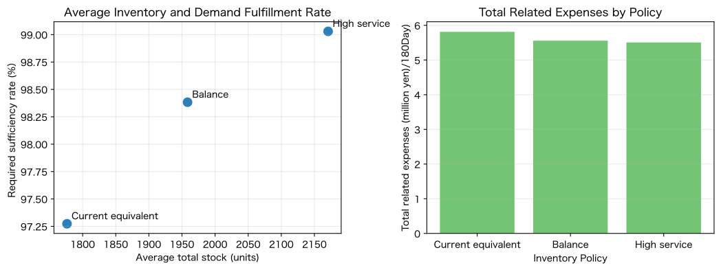
Minimum total related expenses: High service / Fulfillment rate 99.03% / ¥5,506,581

Reading the results

Raising the safety factor increases both the fulfillment rate and the average inventory. While the policy of minimizing total related expenses is a candidate for economic efficiency, sometimes a minimum fulfillment rate that meets customer requirements is set as a constraint first.

In the actual event, in addition to item-specific KPIs, we evaluate emergency orders, on-time delivery, disposal, plan changes, overtime, and equipment load. We check not only averages but also worst weeks and fluctuations.

Practical Implications Seen Through Target Exercise

From No.041 to 050, it is clear that inventory and production policies cannot be determined by a single KPI.

Matching inbounds, sales, out-of-stock, and year-end balances using inventory equations
Break down order points into lead time demand and safety stock
Safety stock is designed based on fluctuations in demand, delivery times, and service levels.
Compare storage costs, out-of-stock costs, and ordering costs on the same scale
Checking the trade-off between lot and inventory with EOQ and the Setup Model
Combining product-specific plans under common equipment and material constraints
Convert lead time shortening into inventory quantity and value
Multi-variety planning treats both minimum supply and economic efficiency simultaneously.
Policies are evaluated using multiple KPIs such as fulfillment rate, inventory, cost, and stability

It’s important not to solve stockouts with inventory alone, but to compare options including forecasts, delivery times, scheduling, capabilities, and outsourcing.

What is necessary for practical implementation

1. Define inventory status and provision rules

Distinguish between cash on hand, reserves, order backlogs, order backlogs, defective pending, and work-in-progress, and standardize the calculation of inventory positions.

2. Create a performance distribution of demand and lead time

It records not only averages but also variations, delays, and consecutive out-of-stock by day, season, customer, and supplier.

3. Agree on cost parameters

Decide on storage costs, capital costs, obsolescence, ordering costs, setup costs, shortage gross profit, urgent transportation, and the scope of customer impact.

4. Properly Model Common Competencies

Equipment, workers, jigs, materials, maintenance, yield, and minimum lot sizes are reflected in the constraints.

5. Backtest policies with historical data

Multiple policies are reproduced within the same demand chain to compare out-of-stock, average inventory, costs, and order frequency.

6. Determine exception handling and renewal responsibilities

Define manual decisions for sudden demand surges, supply stoppages, key customers, and discontinued items, and determine the person responsible and the frequency for updating order points, costs, and capabilities.

Conclusion

No.041–050 used fictitious data of multi-variety replacement parts to confirm the basics of inventory and production models.

Expressing inventory balance using state equations
Designing order points, safety stock, and lots based on demand and lead time
Compare out-of-stock costs, storage costs, ordering costs, and setup costs
Determining multi-variety production volumes under equipment and material constraints
Evaluate policies using multiple KPIs including fulfillment rates, inventory, and costs.

The value of the inventory model lies not in measuring inventory quantities, but in enabling related departments to judge the risk of shortages and the trade-off between capital and capability based on the same premises.

Consultations for Corporations

At Surikoubo, we support the following themes in manufacturing.

Design of order points, safety stock, and order lots
Policy simulation considering out-of-stock and inventory costs
Multi-variety production plans including planning and equipment capacity
Comparison of Lead Time Shortening, Outsourcing, and Overtime Scenarios
Dashboards and operational design for inventory and production KPIs
Actual data-based training for production management, procurement, and DX departments

From the stage of “wanting to reduce inventory but worrying about stockouts” or “having product-specific plans but not fitting into common capabilities,” we can consult from data definition, PoC, and operational design.

📩 Contact Us: surikobo.co.jp/contact Please feel free to consult us first.

Considering stockouts, inventory, planning, and capacity simultaneously: Learning Inventory and Production Modeling through Multi-Variety Replacement Parts

Considering stockouts, inventory, planning, and capabilities simultaneously

Learning Inventory and Production Modeling with Multi-Variety Replacement Parts No.041–No.050

Introduction: Practical Challenges in Manufacturing Covered in This Article

Common situations on site

Why is this issue so difficult to judge?

Overview of Exercise covered this time

Preparing the Python environment

Creation of Fictional Data

No.041: Expressing Changes in Inventory Balance with Formulas

Meaning in Practice

Approach to Analysis and Modeling

Check with Python

Reading the results

No.042: Modeling Order Points

Meaning in Practice

Approach to Analysis and Modeling

Check with Python

Reading the results

No.043: Modeling Safety Stock

Meaning in Practice

Approach to Analysis and Modeling

Check with Python

Reading the results

No.044: Modeling out-of-stock costs and storage costs

Meaning in Practice

Approach to Analysis and Modeling

Check with Python

Reading the results

No.045: Modeling Order Lot Sizes

Meaning in Practice

Approach to Analysis and Modeling

Check with Python

Reading the results

No.046: Modeling Production Capacity Constraints

Meaning in Practice

Approach to Analysis and Modeling

Check with Python

Reading the results

No.047: Modeling Setup Costs

Meaning in Practice

Approach to Analysis and Modeling

Check with Python

Reading the results

No.048: Modeling Lead Time

Meaning in Practice

Approach to Analysis and Modeling

Check with Python

Reading the results

No.049: Modeling Multi-Variety Production Plans

Meaning in Practice

Approach to Analysis and Modeling

Check with Python

Reading the results

No.050: Organizing Evaluation Indicators for Inventory and Production Models

Meaning in Practice

Approach to Analysis and Modeling

Check with Python

Reading the results

Practical Implications Seen Through Target Exercise

What is necessary for practical implementation

1. Define inventory status and provision rules

2. Create a performance distribution of demand and lead time

3. Agree on cost parameters

4. Properly Model Common Competencies

5. Backtest policies with historical data

6. Determine exception handling and renewal responsibilities

Conclusion

Consultations for Corporations

Related Posts

Selecting factory measures to prepare for increased demand based on "profit, delivery time, and risk"

Allocate limited equipment, personnel, and budget to the most valuable work

Predicting the "next state" of equipment, customers, and inventory

Turning demand fluctuations and equipment failures into decision-making based on 'probability'

Turning Waiting for Inspections into Staffing Decisions: Modeling Queues and Congestion Learned in Final Factory Inspection Processes