Allocate limited equipment, personnel, and budget to the most valuable work

Modeling for Optimization Learning at Precision Parts Factories No.081–No.090

In this article, we define product-specific production volume, equipment startup, inspector shifts, delivery routes, and improvement investments as decision variables, optimizing them under objective functions and constraints. Using SciPy, linear programming, integer planning, and binary selection are performed, and the results are translated into on-site instructions and risks.

[!NOTE] This material is a notebook previously used by Surikoubo (or personally by the representative, Kazuyama), and has been reconstructed, edited, and published with the company’s permission. All data listed is fictional and has no relation whatsoever to real companies, factories, or figures.

Introduction: Practical Challenges in Manufacturing Covered in This Article

In a fictional precision parts factory, products A, B, and C share common equipment, personnel, and materials. There is no capacity to meet all demands, so production volumes and product launches must be selected. Additionally, you must decide on the assignment of inspectors by day of the week, deliver to customers on a mobile basis, and allocate investments for DX improvement projects.

Optimization is not magic that automatically gives the right answer. This is decision support that involves agreeing on variables, evaluation criteria, and conditions to be met, and confirming whether the resulting solution is feasible on site.

Common situations on site

• The target products and evaluation criteria for ‘making as much as possible’ are ambiguous
• Meeting equipment schedules but overlooking material and personnel constraints
• Producing fractional production numbers or 0.4 people is an unfeasible solution
• Handling setup costs incurred when producing even one product is handled continuously
• Shift management, delivery, and investment decisions are made solely based on the experience of the person in charge
• Only the optimal value is reported, with no constraints or alternatives presented.

Why is this issue so difficult to judge?

Multiple products compete for common resources, leading to trade-offs in profit, delivery time, and fairness. Values that cannot be included in objective functions are not optimized, and field conditions that cannot be constrained cannot be met.

We adjust continuous variables, integer variables, and binary variables to fit the nature of the work, and check the impact and constraints when the solution changes slightly.

Overview of Exercise covered this time

No.	Theme	Factory Judgment
081	decision variable	What the model decides
082	objective function	What to maximize or minimize
083	Constraint	What must be protected?
084	linear programming	How to allocate production volume by product
085	integer variable	Handling count and number of people as integers
086	binary variable	Handling whether or not a product has been launched
087	Shift	Meeting the required number of people by day of the week
088	Delivery	Shorten the patrol distance
089	budget allocation	Select improvement projects
090	Result translation	Turning the optimal solution into execution instructions

Preparing the Python environment

No external data is used. I use SciPy’s linprog and milp, NumPy, pandas, and matplotlib.

%matplotlib inline
%config InlineBackend.figure_format = 'svg'
import itertools,platform,sys
import matplotlib, matplotlib.pyplot as plt
from matplotlib import font_manager
import numpy as np,pandas as pd,scipy
from scipy.optimize import linprog,milp,Bounds,LinearConstraint
from IPython.display import display

SEED=42; rng=np.random.default_rng(SEED)
fonts={f.name for f in font_manager.fontManager.ttflist}; plot_font=next((f for f in ["Hiragino Sans","Yu Gothic","Noto Sans CJK JP"] if f in fonts),"sans-serif")
plt.rcParams["font.family"]=plot_font; plt.rcParams["axes.unicode_minus"]=False
print(f"Python {sys.version.split()[0]} / NumPy {np.__version__} / pandas {pd.__version__} / SciPy {scipy.__version__}")
print(f"matplotlib {matplotlib.__version__} / font {plot_font} / seed {SEED} / {platform.platform()}")

Python 3.13.1 / NumPy 2.5.1 / pandas 3.0.3 / SciPy 1.18.0
matplotlib 3.11.0 / font Hiragino Sans / seed 42 / macOS-26.3-arm64-arm-64bit-Mach-O

Creation of Fictional Data

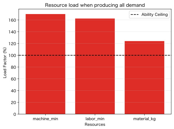
3. Define the product’s marginal profit, equipment time, working time, materials, demand ceiling, minimum supply, and startup fixed costs. The weekly capacity is 6,000 minutes of equipment, 3,300 minutes of work, and 2,250 kg of materials.

products = pd.DataFrame(
    {
        "product": ["A", "B", "C"],
        "margin": [1800, 2700, 4400],
        "machine_min": [4, 7, 12],
        "labor_min": [2, 4, 6],
        "material_kg": [1.2, 1.8, 3.2],
        "demand_max": [800, 520, 280],
        "minimum_supply": [400, 250, 120],
        "setup_cost": [180000, 260000, 420000],
    }
)
capacities = {"machine_min": 6000, "labor_min": 3300, "material_kg": 2250}
display(products.style.format({"margin": "¥{:,.0f}", "setup_cost": "¥{:,.0f}"}))
print("weekly ability:", capacities)

	product	margin	machine_min	labor_min	material_kg	demand_max	minimum_supply	setup_cost
0	A	¥1,800	4	2	1.200000	800	400	¥180,000
1	B	¥2,700	7	4	1.800000	520	250	¥260,000
2	C	¥4,400	12	6	3.200000	280	120	¥420,000

Weekly stats: {'machine_min': 6000, 'labor_min': 3300, 'material_kg': 2250}

full = products.copy()
for resource in capacities:
    full[resource + "_use"] = full[resource] * full["demand_max"]
resource_table = pd.DataFrame(
    {
        "Resources": list(capacities),
        "Total usage when needed": [full[r + "_use"].sum() for r in capacities],
        "Ability": list(capacities.values()),
    }
)
resource_table["load factor"] = resource_table["Total usage when needed"] / resource_table["Ability"]
display(resource_table.style.format({"load factor": "{:.1%}"}))
fig, ax = plt.subplots()
ax.bar(resource_table["Resources"], resource_table["load factor"] * 100, color="#de2d26")
ax.axhline(100, color="black", linestyle="--", label="Ability Ceiling")
ax.set_title("Resource load when producing all demand")
ax.set_xlabel("Resources")
ax.set_ylabel("Load Factor (%）")
ax.grid(True, axis="y", alpha=0.3)
ax.legend()
plt.tight_layout()
plt.show()

	Resources	Total usage when needed	Ability	load factor
0	machine_min	10200.000000	6000	170.0%
1	labor_min	5360.000000	3300	162.4%
2	material_kg	2792.000000	2250	124.1%

---

No.081: Defining Decision Variables

Meaning in Practice

Decision variables are values that the model can select. Define production volume, number of people, and whether the project is launched, as the range within which the person in charge can change.

Approach to Analysis and Modeling

$x_p$ is the weekly production volume of product $p$, and $x_A,x_B,x_C\ge0$. Clearly indicate the unit, time granularity, and the distinction between continuous and integer numbers.

Check with Python

variables = pd.DataFrame(
    {
        "variable": ["x_A", "x_B", "x_C"],
        "Meaning": ["ProductsAProduction volume", "ProductsBProduction volume", "ProductsCProduction volume"],
        "Unit": ["units/week"] * 3,
        "lower limit": products["minimum_supply"],
        "upper limit": products["demand_max"],
        "type": ["continuous (later intigmatized)"] * 3,
    }
)
display(variables)
candidate = np.array([600, 400, 200])
check = products[["machine_min", "labor_min", "material_kg"]].T @ candidate
print("Candidate Plan", dict(zip(products["product"], candidate)), "Resource Use", check.to_dict())

	variable	Meaning	Unit	lower limit	upper limit	type
0	x_A	ProductsAProduction volume	units/week	400	800	continuous (later intigmatized)
1	x_B	ProductsBProduction volume	units/week	250	520	continuous (later intigmatized)
2	x_C	ProductsCProduction volume	units/week	120	280	continuous (later intigmatized)

Candidate Plan {'A': np.int64(600), 'B': np.int64(400), 'C': np.int64(200)} Resource usage {'machine_min': 7600.0, 'labor_min': 4000.0, 'material_kg': 2080.0}

Reading the results

The variable table allows you to separate the range determined by the model from the parameters input by the field. The minimum supply is not a variable, but a constraint.

---

No.082: Defining the Objective Function

Meaning in Practice

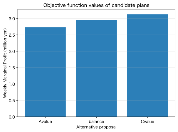
The objective function converts the desirability of a candidate into a single measure. This time, we will maximize the weekly marginal profit.

Approach to Analysis and Modeling

$\max Z=1800x_A+2700x_B+4400x_C$。 To ensure quality, delivery time, and fairness are not ignored, necessary conditions are included as constraints and penalties.

Check with Python

candidates = pd.DataFrame(
    {"case": ["Avalue", "balance", "Cvalue"], "A": [750, 600, 450], "B": [300, 400, 450], "C": [130, 180, 250]}
)
candidates["marginal interest"] = candidates[["A", "B", "C"]].to_numpy() @ products["margin"].to_numpy()
display(candidates.style.format({"marginal interest": "¥{:,.0f}"}))
fig, ax = plt.subplots()
ax.bar(candidates["case"], candidates["marginal interest"] / 1e6, color="#2c7fb8")
ax.set_title("Objective function values of candidate plans")
ax.set_xlabel("Alternative proposal")
ax.set_ylabel("Weekly Marginal Profit (million yen)")
ax.grid(True, axis="y", alpha=0.3)
plt.tight_layout()
plt.show()

	case	A	B	C	marginal interest
0	Avalue	750	300	130	¥2,732,000
1	balance	600	400	180	¥2,952,000
2	Cvalue	450	450	250	¥3,125,000

Reading the results

Even if the profit is high, if it violates restrictions, it cannot be hired. Check the objective function and executability separately.

---

No.083: Defining Constraints

Meaning in Practice

Formulating equipment, personnel, materials, demand, and minimum supply to exclude unfeasible proposals.

Approach to Analysis and Modeling

$\sum_pt_{rp}x_p\le C_r$、$l_p\le x_p\le u_p$。 Align units and distinguish between hard constraints and mitigable targets.

Check with Python

A = products[["machine_min", "labor_min", "material_kg"]].T.to_numpy()
b = np.array(list(capacities.values()))
rows = []
for _, row in candidates.iterrows():
    x = row[["A", "B", "C"]].to_numpy(dtype=float)
    use = A @ x
    rows.append(
        {
            "case": row["case"],
            "Facility capacity": b[0] - use[0],
            "work capacity": b[1] - use[1],
            "Material Availability": b[2] - use[2],
            "executable": bool(np.all(use <= b)),
        }
    )
feasibility = pd.DataFrame(rows)
display(feasibility.style.format({"Facility capacity": "{:+,.0f}", "work capacity": "{:+,.0f}", "Material Availability": "{:+,.0f}"}))

	case	Facility capacity	work capacity	Material Availability	executable
0	Avalue	-660	-180	+394	False
1	balance	-1,360	-580	+234	False
2	Cvalue	-1,950	-900	+100	False

Reading the results

Negative residual power is a violation of constraints. Constraint-specific margin indicates which resources need to be added to make the plan feasible.

---

No.084: Formulating as a Linear Programming Problem

Meaning in Practice

With linear profits and resource constraints, linear planning enables rapid optimal production allocation.

Approach to Analysis and Modeling

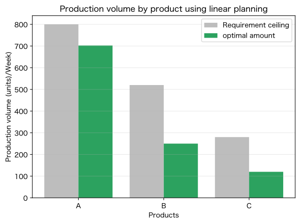
Since SciPy minimizes profit, it sets the profit coefficient to negative. The demand ceiling and minimum supply are set at the variable boundary.

Check with Python

margin = products["margin"].to_numpy()
bounds = list(zip(products["minimum_supply"], products["demand_max"]))
lp = linprog(-margin, A_ub=A, b_ub=b, bounds=bounds, method="highs")
lp_plan = pd.DataFrame({"Products": products["product"], "Production volume": lp.x, "Requirement ceiling": products["demand_max"]})
display(lp_plan.style.format({"Production volume": "{:,.1f}", "Requirement ceiling": "{:,.0f}"}))
print(f"Maximum Weekly Marginal Profit: ¥{-lp.fun:,.0f}")
fig, ax = plt.subplots()
x = np.arange(3)
ax.bar(x - 0.2, lp_plan["Requirement ceiling"], 0.4, label="Requirement ceiling", color="#bdbdbd")
ax.bar(x + 0.2, lp_plan["Production volume"], 0.4, label="optimal amount", color="#2ca25f")
ax.set_xticks(x, lp_plan["Products"])
ax.set_title("Production volume by product using linear planning")
ax.set_xlabel("Products")
ax.set_ylabel("Production volume (units)/Week)")
ax.grid(True, axis="y", alpha=0.3)
ax.legend()
plt.tight_layout()
plt.show()

	Products	Production volume	Requirement ceiling
0	A	702.5	800
1	B	250.0	520
2	C	120.0	280

Maximum Weekly Marginal Profit: ¥2,467,500

Reading the results

This allocation is based on a combination of marginal profit and resource consumption. Remainders are the result of continuous relaxation, and integers are necessary to convert the actual quantity or lot size.

---

No.085: Expressing the Number of Numbers or People Using Integer Variables

Meaning in Practice

The number of products, number of pallets, and number of people are integers. Solve with integer programming so you don’t break constraints with simple rounding.

Approach to Analysis and Modeling

$x_p\in\mathbb{Z}_{\ge0}$ and pass the same objective and constraint to the mixed integer program.

Check with Python

integer = milp(
    c=-margin,
    integrality=np.ones(3),
    bounds=Bounds(products["minimum_supply"], products["demand_max"]),
    constraints=LinearConstraint(A, -np.inf, b),
)
integer_plan = pd.DataFrame({"Products": products["product"], "continuous solution": lp.x, "integer solution": integer.x})
display(integer_plan.style.format({"continuous solution": "{:.2f}", "integer solution": "{:.0f}"}))
print(f"integer solution benefit: ¥{-integer.fun:,.0f} / Difference from continuous solutions: ¥{(-lp.fun)-(-integer.fun):,.0f}")

	Products	continuous solution	integer solution
0	A	702.50	702
1	B	250.00	250
2	C	120.00	120

Integer solution profit: ¥2,466,600 / Difference from continuous solution: ¥900

Reading the results

The integer solution returns the number of executable numbers. The difference from continuous solutions is a trade-off for integer reduction; in lot units, variables are defined as lot numbers.

---

No.086: Expressing Choices Using Binary Variables

Meaning in Practice

When a product is manufactured and a fixed setup fee is incurred, the startup status is expressed as 0/1.

Approach to Analysis and Modeling

$y_p\in\{0,1\}$, as $x_p\le M_py_p$, if there is no production, it is $x_p=0$. Add $-F_py_p$ fixed costs to the purpose.

Check with Python

M = products["demand_max"].to_numpy()
fixed = products["setup_cost"].to_numpy()
c_bin = np.r_[-margin, fixed]
A_res = np.c_[A, np.zeros((3, 3))]
A_link = np.c_[np.eye(3), -np.diag(M)]
A_bin = np.vstack([A_res, A_link])
ub = np.r_[b, np.zeros(3)]
binary = milp(
    c=c_bin,
    integrality=np.ones(6),
    bounds=Bounds(np.zeros(6), np.r_[M, np.ones(3)]),
    constraints=LinearConstraint(A_bin, -np.inf, ub),
)
binary_plan = pd.DataFrame(
    {"Products": products["product"], "Production volume": binary.x[:3], "Startup": binary.x[3:].round().astype(int), "fixed cost": fixed}
)
display(binary_plan.style.format({"Production volume": "{:,.0f}", "fixed cost": "¥{:,.0f}"}))
print(f"Profit after deducting fixed costs: ¥{-binary.fun:,.0f}")

	Products	Production volume	Startup	fixed cost
0	A	800	1	¥180,000
1	B	400	1	¥260,000
2	C	0	0	¥420,000

Profit after fixed fees: ¥2,080,000

Reading the results

For products with high fixed costs, it may be advantageous not to start them up rather than for small-batch production. Big-M uses reasonably small values, such as demand ceilings.

---

No.087: Formulating the Shift Creation Problem

Meaning in Practice

To meet the required number of employees for each day of the week, inspectors are assigned to the five-day consecutive work pattern.

Approach to Analysis and Modeling

The number of people per pattern is set as an integer variable, and the total number of people is minimized if the number of people covered on each day exceeds the required number.

Check with Python

days = ["month", "fire", "Water", "wood", "gold", "soil", "days"]
coverage = np.zeros((7, 7), int)
for start in range(7):
    for k in range(5):
        coverage[(start + k) % 7, start] = 1
required = np.array([8, 9, 10, 10, 9, 6, 5])
shift = milp(
    c=np.ones(7),
    integrality=np.ones(7),
    bounds=Bounds(np.zeros(7), np.full(7, np.inf)),
    constraints=LinearConstraint(coverage, required, np.inf),
)
assigned = np.rint(shift.x).astype(int)
actual = coverage @ assigned
shift_table = pd.DataFrame({"day of the week": days, "required number of people": required, "Number of Personnel": actual, "surplus": actual - required})
display(shift_table)
fig, ax = plt.subplots()
x = np.arange(7)
ax.bar(x - 0.2, required, 0.4, label="necessary", color="#bdbdbd")
ax.bar(x + 0.2, actual, 0.4, label="configuration", color="#2c7fb8")
ax.set_xticks(x, days)
ax.set_title("Required number of people and optimal placement by day of the week")
ax.set_xlabel("day of the week")
ax.set_ylabel("Number of Inspectors (persons)")
ax.grid(True, axis="y", alpha=0.3)
ax.legend()
plt.tight_layout()
plt.show()
print(f"Total number of required inspectors: {assigned.sum()}name / Pattern Number of Passengers: {assigned.tolist()}")

	day of the week	required number of people	Number of Personnel	surplus
0	month	8	8	0
1	fire	9	9	0
2	Water	10	10	0
3	wood	10	10	0
4	gold	9	9	0
5	soil	6	6	0
6	days	5	8	3

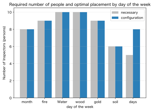
Total number of required inspectors: 12 / Number of pattern members: [3, 1, 3, 0, 2, 0, 3]

Reading the results

This is an integer arrangement that meets the required number of people on all days. Adding desired days off, skills, number of night shifts, and fairness results in a practical shift.

---

No.088: Formulating the Delivery Planning Problem

Meaning in Practice

The distance changes depending on the order in which you visit multiple customers from the factory. List all the small-scale examples and find the shortest route.

Approach to Analysis and Modeling

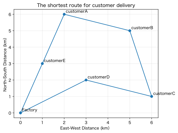
This is the issue of traveling salespeople who leave and return to factories. At 6 locations, you can compare the $5!=120$ routes of 5 customer locations.

Check with Python

locations = pd.DataFrame(
    {"name": ["Factory", "customerA", "customerB", "customerC", "customerD", "customerE"], "x": [0, 2, 5, 6, 3, 1], "y": [0, 6, 5, 1, 2, 3]}
)
xy = locations[["x", "y"]].to_numpy()
dist = np.linalg.norm(xy[:, None, :] - xy[None, :, :], axis=2)
routes = []
for perm in itertools.permutations(range(1, 6)):
    route = (0,) + perm + (0,)
    routes.append((sum(dist[route[i], route[i + 1]] for i in range(6)), route))
best_distance, best_route = min(routes)
names = [locations.iloc[i]["name"] for i in best_route]
print(f"shortest distance: {best_distance:.2f}km / Route: {' → '.join(names)}")
fig, ax = plt.subplots()
route_xy = xy[list(best_route)]
ax.plot(route_xy[:, 0], route_xy[:, 1], marker="o")
for _, r in locations.iterrows():
    ax.annotate(r["name"], (r["x"], r["y"]), xytext=(4, 4), textcoords="offset points")
ax.set_title("The shortest route for customer delivery")
ax.set_xlabel("East-West Distance (km）")
ax.set_ylabel("North-South Distance (km）")
ax.grid(True, alpha=0.3)
plt.tight_layout()
plt.show()

Shortest distance: 20.38km / Route: Factory → Customer D → Customer C → Customer B → Customer A → Customer E → Factory

Reading the results

On a small scale, you can list them all, but increasing the number of points causes combinations to surge. When adding vehicle capacity, time windows, or multiple vehicles, use dedicated solvers or approximate methods.

---

No.089: Formulating the Budget Allocation Problem

Meaning in Practice

Based on the cost, required work, and expected effects of the improvement project, we select the selected project within budget and personnel.

Approach to Analysis and Modeling

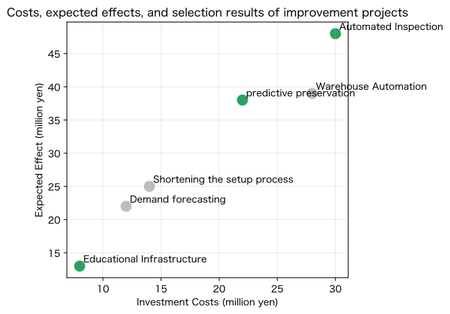
$y_j\in\{0,1\}$ project accepted, $\max\sum_jv_jy_j$ is a 0-to-1 knapsack with budget and labor constraints.

Check with Python

projects = pd.DataFrame(
    {
        "Case": ["predictive preservation", "Automated Inspection", "Shortening the setup process", "Demand forecasting", "Warehouse Automation", "Educational Infrastructure"],
        "Fees_million yen": [22, 30, 14, 12, 28, 8],
        "man-hours_person month": [5, 7, 4, 3, 6, 2],
        "Expected Effects_million yen": [38, 48, 25, 22, 39, 13],
    }
)
A_proj = projects[["Fees_million yen", "man-hours_person month"]].T.to_numpy()
budget = milp(
    c=-projects["Expected Effects_million yen"],
    integrality=np.ones(len(projects)),
    bounds=Bounds(np.zeros(len(projects)), np.ones(len(projects))),
    constraints=LinearConstraint(A_proj, -np.inf, [60, 15]),
)
projects["Adoption"] = np.rint(budget.x).astype(int)
display(projects)
selected = projects.query("`Adoption`==1")
print(
    f"Adoption: {', '.join(selected['Case'])} / Fees {selected['Fees_million yen'].sum()}million yen / Effects {selected['Expected Effects_million yen'].sum()}million yen"
)
fig, ax = plt.subplots()
colors = np.where(projects["Adoption"] == 1, "#2ca25f", "#bdbdbd")
ax.scatter(projects["Fees_million yen"], projects["Expected Effects_million yen"], s=120, c=colors)
for _, r in projects.iterrows():
    ax.annotate(r["Case"], (r["Fees_million yen"], r["Expected Effects_million yen"]), xytext=(4, 4), textcoords="offset points")
ax.set_title("Costs, expected effects, and selection results of improvement projects")
ax.set_xlabel("Investment Costs (million yen)")
ax.set_ylabel("Expected Effect (million yen)")
ax.grid(True, alpha=0.3)
plt.tight_layout()
plt.show()

	Case	Fees_million yen	man-hours_person month	Expected Effects_million yen	Adoption
0	predictive preservation	22	5	38	1
1	Automated Inspection	30	7	48	1
2	Shortening the setup process	14	4	25	0
3	Demand forecasting	12	3	22	0
4	Warehouse Automation	28	6	39	0
5	Educational Infrastructure	8	2	13	1

Adoption: Predictive maintenance, automated inspection, educational infrastructure / Cost: 60 million yen / Effectiveness: 99 million yen

Reading the results

It’s not just a simple cost-effectiveness ratio, but a combination that meets both budget and labor at the same time. Add deal dependency, risk, and strategic mandatory projects.

---

No.090: Translating the results of optimization models into business decisions

Meaning in Practice

Only when optimal values are translated into production instructions, constraints, personnel, delivery, investment, and precautions can they be executed.

Approach to Analysis and Modeling

Summarize the solution, objective value, constraint utilization, capacity, assumptions, and alternatives in a decision table. Confirm sensitivity and site constraints.

Check with Python

xopt = integer.x
uses = A @ xopt
decision_summary = pd.DataFrame(
    {
        "Decision-making": ["ProductsA/B/CProduction", "inspector", "Delivery", "Improved Investment"],
        "Recommendation": [
            f"{xopt[0]:.0f}/{xopt[1]:.0f}/{xopt[2]:.0f}units",
            f"{assigned.sum()}name",
            "→".join(names),
            ", ".join(selected["Case"]),
        ],
        "confirmation item": [
            f"Equipment{uses[0]/b[0]:.1%}・Work{uses[1]/b[1]:.1%}・Ingredients{uses[2]/b[2]:.1%}",
            "Preferred Days Off & Skill Restrictions",
            "Time window and load capacity",
            "Uncertainty of effectiveness and project dependence",
        ],
    }
)
display(decision_summary)
resource_use = pd.DataFrame({"Resources": ["Equipment", "assignment", "Ingredients"], "usage amount": uses, "Ability": b})
resource_use["usage rate"] = resource_use["usage amount"] / resource_use["Ability"]
fig, ax = plt.subplots()
ax.bar(resource_use["Resources"], resource_use["usage rate"] * 100, color="#756bb1")
ax.axhline(100, color="black", linestyle="--")
ax.set_title("Resource Utilization Rate in Optimal Production Planning")
ax.set_xlabel("Resources")
ax.set_ylabel("Usage rate (%）")
ax.grid(True, axis="y", alpha=0.3)
plt.tight_layout()
plt.show()
bottleneck = resource_use.loc[resource_use["usage rate"].idxmax()]
print(f"Most Tight Resources: {bottleneck['Resources']}（{bottleneck['usage rate']:.1%}）")

	Decision-making	Recommendation	confirmation item
0	ProductsA/B/CProduction	702/250/120units	Equipment100.0%・Work94.7%・Ingredients74.5%
1	inspector	12name	Preferred Days Off & Skill Restrictions
2	Delivery	Factory→customerD→customerC→customerB→customerA→customerE→Factory	Time window and load capacity
3	Improved Investment	predictive preservation, Automated Inspection, Educational Infrastructure	Uncertainty of effectiveness and project dependence

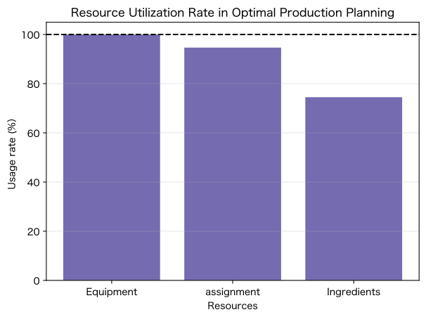
Most scarce resource: Equipment (100.0%)

Reading the results

It shows not only production volume but also bottlenecks and unreflected conditions. Without directly giving instructions on the optimal solution, we conduct on-site reviews of rounding, setup order, quality, delivery time, and resistance to change.

---

Practical Implications Seen Through Target Exercise

In optimization, the definition of decision variables, objective functions, and constraints determines the outcome. Continuous, integers, and binary values can be tailored to each business unit, and shifts, deliveries, and investments can be handled within the same framework. It is important to present not only optimal values but also constraints, assumptions, alternatives, and sensitivities.

What is necessary for practical implementation

1. Decide on the decision-making cycle and units

We unify daily, weekly, individual, lot, and individual numbers.

2. Distinguish between hard constraints and goals

We consider imposing restrictions on safety, laws, and contracts, and penalties on preferred delivery deadlines.

3. Manage parameter bases

Determine the responsible persons for capacity, workload, profit, demand limits, fixed costs, and update frequency.

4. Compare with current plans in parallel

Evaluate not only profits but also the number of changes, overtime, delivery times, and on-site load.

5. Decide on the operation when infeasible

Define which constraints to relax and who approves.

6. Convert the results to executable format

We provide production instructions, shift schedules, delivery sequences, and investment project lists to the site.

Conclusion

No.081–090 represent production volume, startup, shift, delivery, and investment as optimization models. The value of mathematical optimization lies not only in achieving maximum values but also in making trade-offs with resource competition visible and enabling comparison of actionable decisions.

Consultations for Corporations

At Mathematical Laboratory, we support production planning, workforce shifts, delivery, equipment allocation, and investment allocation with mathematical optimization PoCs and operational design.

📩 Contact Us: surikobo.co.jp/contact Please feel free to consult us first.