Turning demand fluctuations and equipment failures into decision-making based on ‘probability’

Modeling Uncertainty and Risk Learning with Critical Replacement Parts No.061–No.070

In this article, we use key replacement parts for hypothetical industrial equipment and heat treatment equipment as subjects, and represent demand, delivery time, yield, and failure timing as random variables. By using expected value, standard deviation, probability distribution, forecast interval, out-of-stock probability, failure probability, and expected loss, risks that cannot be seen by averages alone are connected to inventory and maintenance decisions.

[!NOTE] This material is a notebook previously used by Surikoubo (or personally by the representative, Kazuyama), and has been reconstructed, edited, and published with the company’s permission. All data listed is fictional and has no relation whatsoever to real companies, factories, or figures.

Introduction: Practical Challenges in Manufacturing Covered in This Article

For replacement parts manufacturers, shortages due to surging demand and sudden failures of heat treatment equipment are affecting delivery times. Planning based solely on average demand and mean interval of failure may be efficient under normal conditions, but losses when fluctuations overlap cannot be accounted for.

Using a 365-day product demand and a hypothetical model of equipment lifespan, we simultaneously compare average results and losses during deterioration.

Common situations on site

• Inventory is determined solely by average demand, without monitoring demand variation.
• Treat options with the same expected profit as equal and do not compare the size of the loss.
• Mechanically applying the same normal distribution to quantity, delivery time, and yield
• Presenting sales forecasts as a single numerical value and not submitting forecast ranges to management meetings
• Failure probability and loss during failure are managed separately.
• Only the option with the highest expected value is selected, without checking tolerance for the worst-case scenario.

Why is this issue so difficult to judge?

Uncertainty refers to “values not being fixed,” while risk is “uncertain results leading to operational losses.” It is necessary to compare failures with low probability but significant impact against frequent but minor demand fluctuations using the same criteria.

We check not only averages but also distributions, top quantiles, loss probabilities, expected losses, and averages when things worsen.

Overview of Exercise covered this time

No.	Theme	judgment
061	random variable	How to express demand, delivery dates, and yield
062	expected value	How to compare average results
063	Variance and Standard Deviation	How to measure variation
064	distribution selection	What kind of distribution should match the workload?
065	Demand distribution	How to express lead time demand
066	Sales forecast range	How to show upper and lower sales limits
067	Stockout Probability	What is the risk of stockouts per inventory level?
068	failure probability	What is the probability of failure during the maintenance interval?
069	expected loss	How to integrate probability and impact
070	Decision-making	How to balance expected value with risk in the event of deterioration

Preparing the Python environment

No external data is used. Fix random number seeds and simulate them using NumPy, pandas, SciPy, and matplotlib.

%matplotlib inline
%config InlineBackend.figure_format = 'svg'
import platform, sys
import matplotlib, matplotlib.pyplot as plt
from matplotlib import font_manager
import numpy as np, pandas as pd, scipy
from scipy import stats
from IPython.display import display
SEED=42; rng=np.random.default_rng(SEED)
fonts={f.name for f in font_manager.fontManager.ttflist}
plot_font=next((f for f in ["Hiragino Sans","Yu Gothic","Noto Sans CJK JP"] if f in fonts),"sans-serif")
plt.rcParams["font.family"]=plot_font; plt.rcParams["axes.unicode_minus"]=False
print(f"Python {sys.version.split()[0]} / NumPy {np.__version__} / pandas {pd.__version__} / SciPy {scipy.__version__}")
print(f"matplotlib {matplotlib.__version__} / font {plot_font} / seed {SEED} / {platform.platform()}")

Python 3.13.1 / NumPy 2.5.1 / pandas 3.0.3 / SciPy 1.18.0
matplotlib 3.11.0 / font Hiragino Sans / seed 42 / macOS-26.3-arm64-arm-64bit-Mach-O

Creation of Fictional Data

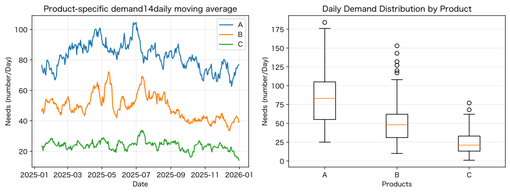
It generates the 365-day demand for products A, B, and C from a negative binomial distribution. Average demand and variance vary by product, and multipliers for days of the week and season are added. The equipment lifespan is based on a Weibull distribution with a shape number of 2.2 and a scale of 420 days.

dates=pd.date_range("2025-01-01",periods=365,freq="D")
specs=pd.DataFrame({"product":["A","B","C"],"mean_demand":[95,58,28],"dispersion":[18,10,5],"price":[5200,8400,14500],"unit_margin":[1800,3100,5600],"shortage_loss":[3500,6000,12000],"lead_days":[5,8,12]})
rows=[]
for i,date in enumerate(dates):
    factor=(.48 if date.dayofweek>=5 else 1.0)*(1+.14*np.sin(2*np.pi*(i-50)/365))
    for s in specs.itertuples(index=False):
        mu=max(1,s.mean_demand*factor); k=s.dispersion; p=k/(k+mu)
        rows.append({"date":date,"product":s.product,"demand":rng.negative_binomial(k,p),"expected":mu})
demand=pd.DataFrame(rows).merge(specs,on="product")
print(f"Demand Data: {len(demand):,}Walk (365days×3Products)")
display(demand.head(9).style.format({"expected":"{:.1f}","price":"¥{:,.0f}"}))

Demand data: 1,095 rows (365 days× 3 products)

	date	product	demand	expected	mean_demand	dispersion	price	unit_margin	shortage_loss	lead_days
0	2025-01-01 00:00:00	A	101	84.9	95	18	¥5,200	1800	3500	5
1	2025-01-01 00:00:00	B	18	51.8	58	10	¥8,400	3100	6000	8
2	2025-01-01 00:00:00	C	37	25.0	28	5	¥14,500	5600	12000	12
3	2025-01-02 00:00:00	A	95	85.1	95	18	¥5,200	1800	3500	5
4	2025-01-02 00:00:00	B	72	51.9	58	10	¥8,400	3100	6000	8
5	2025-01-02 00:00:00	C	45	25.1	28	5	¥14,500	5600	12000	12
6	2025-01-03 00:00:00	A	83	85.2	95	18	¥5,200	1800	3500	5
7	2025-01-03 00:00:00	B	88	52.0	58	10	¥8,400	3100	6000	8
8	2025-01-03 00:00:00	C	23	25.1	28	5	¥14,500	5600	12000	12

summary=demand.groupby("product",as_index=False).agg(average_need=("demand","mean"),standard_deviation=("demand","std"),smallest=("demand","min"),largest=("demand","max"))
display(summary.style.format({"average_need":"{:.1f}","standard_deviation":"{:.1f}"}))
fig,axes=plt.subplots(1,2,figsize=(11,4.2))
for p,g in demand.groupby("product"): axes[0].plot(g["date"],g["demand"].rolling(14).mean(),label=p)
axes[0].set_title("Product-specific demand14daily moving average"); axes[0].set_xlabel("Date"); axes[0].set_ylabel("Needs (number/Day)"); axes[0].grid(True,alpha=.3); axes[0].legend()
axes[1].boxplot([g["demand"] for _,g in demand.groupby("product")],tick_labels=["A","B","C"])
axes[1].set_title("Daily Demand Distribution by Product"); axes[1].set_xlabel("Products"); axes[1].set_ylabel("Needs (number/Day)"); axes[1].grid(True,axis="y",alpha=.3)
plt.tight_layout(); plt.show()

	product	average_need	standard_deviation	smallest	largest
0	A	82.4	32.5	25	184
1	B	48.9	23.5	10	153
2	C	23.7	13.9	1	77

---

No.061: Expressing Uncertainty as a Random Variable

Meaning in Practice

Expressing demand, lead time, yield, and lifespan as random variables rather than fixed values allows you to handle multiple outcomes and likelihood of occurrence.

Approach to Analysis and Modeling

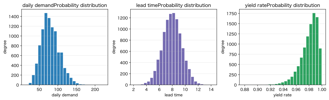
$X:\Omega\to\mathbb{R}$ is used as a random variable, and the demand $D$, delivery $L$, and yield $Y$ are represented as distributions. Decide the units and the range you can take first.

Check with Python

samples=pd.DataFrame({"daily demand":rng.negative_binomial(12,12/(12+80),10000),"lead time":np.maximum(1,rng.normal(8,1.5,10000)),"yield rate":rng.beta(98,2,10000)})
display(samples.describe(percentiles=[.05,.5,.95]).T.style.format("{:.2f}"))
fig,axes=plt.subplots(1,3,figsize=(12,3.7))
for ax,col,color in zip(axes,samples.columns,["#2c7fb8","#756bb1","#2ca25f"]):
    ax.hist(samples[col],bins=25,color=color,edgecolor="white"); ax.set_title(col+"Probability distribution"); ax.set_xlabel(col); ax.set_ylabel("degree"); ax.grid(True,axis="y",alpha=.3)
plt.tight_layout(); plt.show()

	count	mean	std	min	5%	50%	95%	max
daily demand	10000.00	80.02	24.70	13.00	43.00	77.00	124.00	224.00
lead time	10000.00	7.98	1.49	2.14	5.53	7.98	10.48	14.28
yield rate	10000.00	0.98	0.01	0.88	0.95	0.98	1.00	1.00

Reading the results

Demand is a non-negative integer, delivery time is a positive continuous value, and yield is 0–1. Choosing a distribution that fits the workload range is the premise for realistic simulation.

---

No.062: Expressing Average Results Using Expected Values

Meaning in Practice

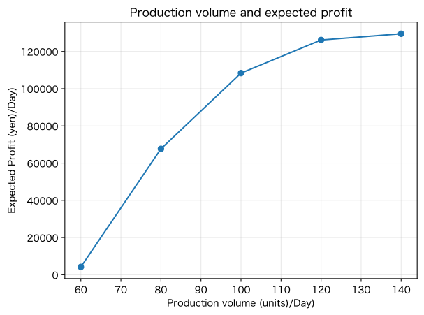
You can compare the average profit for each production volume candidate. However, you cannot determine the range of losses based solely on expected values.

Approach to Analysis and Modeling

$E[X]=\sum_x xP(X=x)$ is here. Monte Carlo evaluates profits after subtracting unsold expenses and out-of-stock losses from profits that meet demand.

Check with Python

d_sim=rng.choice(demand.query("product=='A'")["demand"],size=30000,replace=True)
plans=[]
for q in [60,80,100,120,140]:
    sold=np.minimum(q,d_sim); leftover=np.maximum(q-d_sim,0); shortage=np.maximum(d_sim-q,0)
    profit=sold*1800-leftover*250-shortage*3500
    plans.append({"Production volume":q,"expected benefit":profit.mean(),"probability of loss":(profit<0).mean(),"5%point":np.quantile(profit,.05)})
ev=pd.DataFrame(plans); display(ev.style.format({"expected benefit":"¥{:,.0f}","probability of loss":"{:.1%}","5%point":"¥{:,.0f}"}))
fig,ax=plt.subplots(); ax.plot(ev["Production volume"],ev["expected benefit"],marker="o"); ax.set_title("Production volume and expected profit"); ax.set_xlabel("Production volume (units)/Day)"); ax.set_ylabel("Expected Profit (yen)/Day)"); ax.grid(True,alpha=.3); plt.tight_layout(); plt.show()

	Production volume	expected benefit	probability of loss	5%point
0	60	¥4,188	39.9%	¥-154,500
1	80	¥67,665	12.0%	¥-48,500
2	100	¥108,383	2.3%	¥32,400
3	120	¥126,173	0.3%	¥35,600
4	140	¥129,515	0.0%	¥32,650

Reading the results

The plan with the highest expected profit is generally advantageous, but also check the 5% point and loss probability. Your choice depends on your financial capacity and the importance of your customers.

---

No.063: Expressing Variance with Variance and Standard Deviation

Meaning in Practice

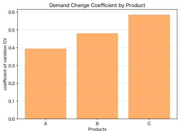
Even if average demand is the same, products with larger standard deviations require safety stock and capacity margins.

Approach to Analysis and Modeling

$\mathrm{Var}(X)=E[(X-\mu)^2]$、$\sigma=\sqrt{\mathrm{Var}(X)}$。 Scale is adjusted with a coefficient of variation $CV=\sigma/\mu$.

Check with Python

variability=demand.groupby("product")["demand"].agg(["mean","var","std"]).reset_index(); variability["CV"]=variability["std"]/variability["mean"]
display(variability.style.format({"mean":"{:.1f}","var":"{:.1f}","std":"{:.1f}","CV":"{:.2f}"}))
fig,ax=plt.subplots(); ax.bar(variability["product"],variability["CV"],color="#fdae6b"); ax.set_title("Demand Change Coefficient by Product"); ax.set_xlabel("Products"); ax.set_ylabel("coefficient of variation CV"); ax.grid(True,axis="y",alpha=.3); plt.tight_layout(); plt.show()

	product	mean	var	std	CV
0	A	82.4	1057.0	32.5	0.39
1	B	48.9	552.5	23.5	0.48
2	C	23.7	192.7	13.9	0.59

Reading the results

Standard deviation is in units of the original quantity, variance is the square of the quantity, and CV is ununited. CV is useful for comparing different demand scales.

---

No.064: Selecting a Probability Distribution That Fits Business Data

Meaning in Practice

The range and generation process differ depending on the quantity, duration, ratio, and lifespan. Incorrect selection of distribution leads to negative demand and yields exceeding 100%.

Approach to Analysis and Modeling

For case count, candidates are Poisson and negative binomial; for positive time, gamma and log-normal; for ratio, beta; and for lifespan, Weibull. Choose based on mean and variance, histogram, and business knowledge.

Check with Python

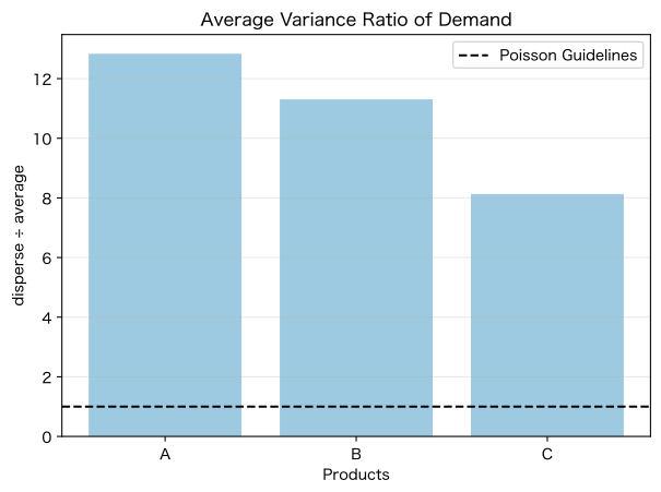
dist_check=demand.groupby("product")["demand"].agg(["mean","var"]).reset_index(); dist_check["mean ratio of variance"]=dist_check["var"]/dist_check["mean"]; dist_check["Candidate"] = np.where(dist_check["mean ratio of variance"]>1.3,"Negative binomial distribution","Poisson distribution")
display(dist_check.style.format({"mean":"{:.1f}","var":"{:.1f}","mean ratio of variance":"{:.2f}"}))
fig,ax=plt.subplots(); ax.bar(dist_check["product"],dist_check["mean ratio of variance"],color="#9ecae1"); ax.axhline(1,color="black",linestyle="--",label="Poisson Guidelines"); ax.set_title("Average Variance Ratio of Demand"); ax.set_xlabel("Products"); ax.set_ylabel("disperse ÷ average"); ax.grid(True,axis="y",alpha=.3); ax.legend(); plt.tight_layout(); plt.show()

	product	mean	var	mean ratio of variance	Candidate
0	A	82.4	1057.0	12.84	Negative binomial distribution
1	B	48.9	552.5	11.30	Negative binomial distribution
2	C	23.7	192.7	8.13	Negative binomial distribution

Reading the results

The variance is significantly above the average and is more overdistributed than simple Poissons. A negative binomial distribution that can represent surges in demand or customer gaps is a candidate.

---

No.065: Expressing Demand as a Probability Distribution

Meaning in Practice

By creating a distribution of lead time demand, you can determine order points based on quantiles rather than averages.

Approach to Analysis and Modeling

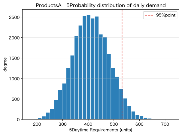
$D_L=\sum_{t=1}^L D_t$ is simulated using historical reextraction, and the average score of 95% and 99% is calculated.

Check with Python

a_hist=demand.query("product=='A'")["demand"].to_numpy(); lead=5
lead_demand=rng.choice(a_hist,size=(30000,lead),replace=True).sum(axis=1)
lead_kpi=pd.DataFrame({"average":[lead_demand.mean()],"standard_deviation":[lead_demand.std()],"95%point":[np.quantile(lead_demand,.95)],"99%point":[np.quantile(lead_demand,.99)]})
display(lead_kpi.style.format("{:.0f}units"))
fig,ax=plt.subplots(); ax.hist(lead_demand,bins=35,color="#2c7fb8",edgecolor="white"); ax.axvline(np.quantile(lead_demand,.95),color="#de2d26",linestyle="--",label="95%point"); ax.set_title("ProductsA：5Probability distribution of daily demand"); ax.set_xlabel("5Daytime Requirements (units)"); ax.set_ylabel("degree"); ax.grid(True,axis="y",alpha=.3); ax.legend(); plt.tight_layout(); plt.show()

	average	standard_deviation	95%point	99%point
0	411units	72units	532units	583units

Reading the results

In average inventory, it exceeds in about half the cases. Quantiles corresponding to the target service level are selected as order point candidates.

---

No.066: Modeling Sales Forecast Ranges

Meaning in Practice

By not showing sales as a single point but showing forecast ranges through demand, price, and yield, you can scenario capital and capacity planning.

Approach to Analysis and Modeling

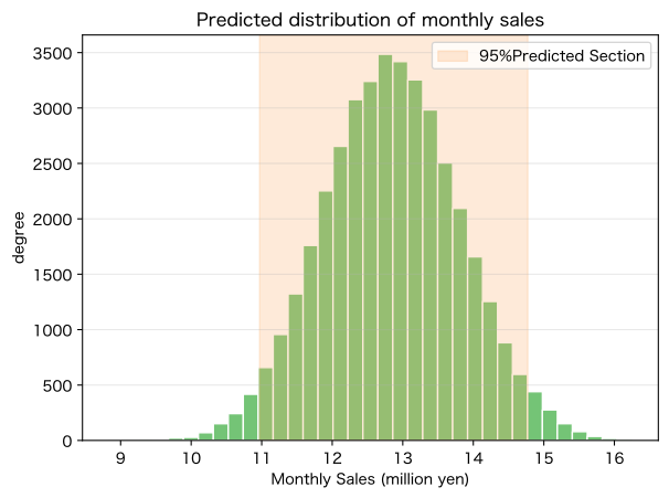
Calculate monthly sales $R=P\min(D,QY)$ Monte Carlo to obtain the median and the 80%/95% range.

Check with Python

n=40000; monthly_demand=rng.choice(a_hist,size=(n,30),replace=True).sum(axis=1); price=rng.normal(5200,120,n); yield_rate=rng.beta(98,2,n); capacity=3000
revenue=price*np.minimum(monthly_demand,capacity*yield_rate)
qs=np.quantile(revenue,[.025,.1,.5,.9,.975]); interval=pd.DataFrame({"indicator":["2.5%","10%","median","90%","97.5%"],"Monthly Sales":qs}); display(interval.style.format({"Monthly Sales":"¥{:,.0f}"}))
fig,ax=plt.subplots(); ax.hist(revenue/1e6,bins=35,color="#74c476",edgecolor="white"); ax.axvspan(qs[0]/1e6,qs[-1]/1e6,color="#fdae6b",alpha=.25,label="95%Predicted Section"); ax.set_title("Predicted distribution of monthly sales"); ax.set_xlabel("Monthly Sales (million yen)"); ax.set_ylabel("degree"); ax.grid(True,axis="y",alpha=.3); ax.legend(); plt.tight_layout(); plt.show()
print(f"95%Predicted Section: ¥{qs[0]:,.0f}〜¥{qs[-1]:,.0f}")

	indicator	Monthly Sales
0	2.5%	¥10,969,947
1	10%	¥11,602,134
2	median	¥12,838,050
3	90%	¥14,095,645
4	97.5%	¥14,773,267

95% Forecast Range: ¥10,969,947 to ¥14,773,267

Reading the results

The forecast range includes not only demand but also uncertainties in price and yield. Use the lower limit for cash flow and the upper limit for capacity planning.

---

No.067: Expressing Out-of-Stock Risk in Probabilistic Terms

Meaning in Practice

By showing the probability of out-of-stock during lead time at each inventory level, you can explain the trade-off between inventory and service.

Approach to Analysis and Modeling

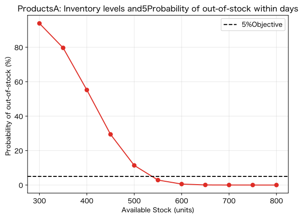
$P(\mathrm{stockout})=P(D_L>I)$ is estimated through simulation.

Check with Python

stock_levels=np.arange(300,801,50); risk=pd.DataFrame({"Inventory":stock_levels,"Stockout Probability":[np.mean(lead_demand>s) for s in stock_levels]}); display(risk.style.format({"Stockout Probability":"{:.1%}"}))
fig,ax=plt.subplots(); ax.plot(risk["Inventory"],risk["Stockout Probability"]*100,marker="o",color="#de2d26"); ax.axhline(5,color="black",linestyle="--",label="5%Objective"); ax.set_title("ProductsA: Inventory levels and5Probability of out-of-stock within days"); ax.set_xlabel("Available Stock (units)"); ax.set_ylabel("Probability of out-of-stock (%）"); ax.grid(True,alpha=.3); ax.legend(); plt.tight_layout(); plt.show()
target_stock=risk.loc[risk["Stockout Probability"]<=.05,"Inventory"].min(); print(f"Stockout Probability5%The following are the smallest candidates:: {target_stock:.0f}units")

	Inventory	Stockout Probability
0	300	93.9%
1	350	79.6%
2	400	55.2%
3	450	29.4%
4	500	11.4%
5	550	2.9%
6	600	0.6%
7	650	0.1%
8	700	0.0%
9	750	0.0%
10	800	0.0%

Minimum candidate with a shortage probability of 5% or less: 550 units

Reading the results

Increasing inventory lowers the probability of stockouts, but marginal improvement gradually diminishes. Combine target probabilities and storage costs by importance level.

---

No.068: Expressing Failure Risk in Probabilities

Meaning in Practice

Expressing equipment lifespan as a probability distribution allows for quantifying the probability of failure before the next maintenance.

Approach to Analysis and Modeling

The cumulative failure probability of the Weibull distribution is $F(t)=1-\exp[-(t/\eta)^\beta]$. $\beta>1$ is a type of aging type.

Check with Python

beta,eta=2.2,420; days=np.arange(30,601,30); failure_prob=1-np.exp(-(days/eta)**beta); failure=pd.DataFrame({"maintenance interval_days":days,"Probability of failure within the period":failure_prob}); display(failure.iloc[::2].style.format({"Probability of failure within the period":"{:.1%}"}))
fig,ax=plt.subplots(); ax.plot(days,failure_prob*100,marker="o",color="#756bb1"); ax.axhline(10,color="black",linestyle="--",label="10%guideline"); ax.set_title("Maintenance intervals and failure probability within the period"); ax.set_xlabel("Maintenance interval (days)"); ax.set_ylabel("Failure probability (%）"); ax.grid(True,alpha=.3); ax.legend(); plt.tight_layout(); plt.show()
limit=failure.loc[failure["Probability of failure within the period"]<=.10,"maintenance interval_days"].max(); print(f"failure probability10%The following are the maximum spacing candidates:: {limit}days")

	maintenance interval_days	Probability of failure within the period
0	30	0.3%
2	90	3.3%
4	150	9.9%
6	210	19.6%
8	270	31.5%
10	330	44.5%
12	390	57.2%
14	450	68.8%
16	510	78.4%
18	570	85.9%

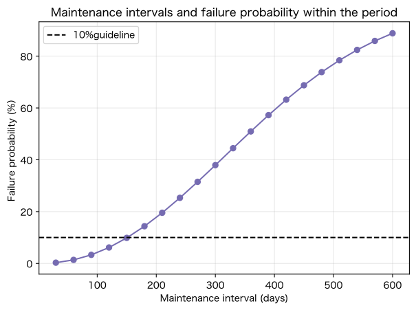
Maximum interval candidate with failure probability below 10%: 150 days

Reading the results

The longer the maintenance interval, the higher the probability of failure. We update the number by product group based on actual failures and replacement histories, and compare them with preventive replacement costs.

---

No.069: Using Expected Loss to Assess Risk

Meaning in Practice

By multiplying the probability of occurrence by the impact amount, different types of risks can be prioritized on a common monetary scale.

Approach to Analysis and Modeling

$EL=\sum_jp_jL_j$。 However, low-frequency large losses confirm not only expectations but also maximum losses and business continuity constraints.

Check with Python

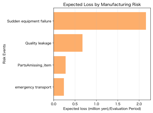
risks=pd.DataFrame({"Risks":["PartsAmissing_item","Sudden equipment failure","Quality leakage","emergency transport"],"Probability of occurrence":[.08,.12,.015,.20],"Impact amount":[3_500_000,18_000_000,45_000_000,1_200_000]}); risks["expected loss"]=risks["Probability of occurrence"]*risks["Impact amount"]; risks=risks.sort_values("expected loss",ascending=False); display(risks.style.format({"Probability of occurrence":"{:.1%}","Impact amount":"¥{:,.0f}","expected loss":"¥{:,.0f}"}))
fig,ax=plt.subplots(); ax.barh(risks["Risks"][::-1],risks["expected loss"][::-1]/1e6,color="#fdae6b"); ax.set_title("Expected Loss by Manufacturing Risk"); ax.set_xlabel("Expected loss (million yen)/Evaluation Period)"); ax.set_ylabel("Risk Events"); ax.grid(True,axis="x",alpha=.3); plt.tight_layout(); plt.show()

	Risks	Probability of occurrence	Impact amount	expected loss
1	Sudden equipment failure	12.0%	¥18,000,000	¥2,160,000
2	Quality leakage	1.5%	¥45,000,000	¥675,000
0	PartsAmissing_item	8.0%	¥3,500,000	¥280,000
3	emergency transport	20.0%	¥1,200,000	¥240,000

Reading the results

You can compare high-probability/medium losses and low-probability/massive losses in the same table. Unacceptable risks such as quality leaks are treated as constraints regardless of expected loss ranking.

---

No.070: Organizing Decisions Considering Uncertainty

Meaning in Practice

A plan with a low expected cost and a strong one when the situation worsens do not match. Select your policy by listing both the average and tail risk.

Approach to Analysis and Modeling

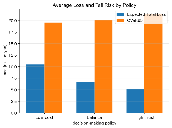
Calculate total losses for each inventory and maintenance policy in Monte Carlo, and compare expected losses, 95% points, and the worst average CVaR of 5%.

Check with Python

decisions=[]; n=30000
for name,stock,interval,annual_cost in [("Low cost",450,360,1_200_000),("Balance",550,240,2_100_000),("High Trust",650,150,3_400_000)]:
    dl=rng.choice(a_hist,size=(n,5),replace=True).sum(axis=1); shortage=np.maximum(dl-stock,0)*3500
    fail=rng.random(n)<(1-np.exp(-(interval/eta)**beta)); failure_loss=fail*18_000_000
    total=annual_cost+shortage+failure_loss; q95=np.quantile(total,.95); cvar=total[total>=q95].mean()
    decisions.append({"policy":name,"Expected Total Loss":total.mean(),"95%point":q95,"CVaR95":cvar,"loss500Over 10,000 yen odds":np.mean(total>5_000_000)})
decision=pd.DataFrame(decisions); display(decision.style.format({"Expected Total Loss":"¥{:,.0f}","95%point":"¥{:,.0f}","CVaR95":"¥{:,.0f}","loss500Over 10,000 yen odds":"{:.1%}"}))
fig,ax=plt.subplots(); x=np.arange(3); ax.bar(x-.18,decision["Expected Total Loss"]/1e6,.36,label="Expected Total Loss"); ax.bar(x+.18,decision["CVaR95"]/1e6,.36,label="CVaR95"); ax.set_xticks(x,decision["policy"]); ax.set_title("Average Loss and Tail Risk by Policy"); ax.set_xlabel("decision-making policy"); ax.set_ylabel("Loss (million yen)"); ax.grid(True,axis="y",alpha=.3); ax.legend(); plt.tight_layout(); plt.show()
best=decision.loc[decision["Expected Total Loss"].idxmin()]; print(f"Minimum expected total loss: {best['policy']} / ¥{best['Expected Total Loss']:,.0f}")

	policy	Expected Total Loss	95%point	CVaR95	loss500Over 10,000 yen odds
0	Low cost	¥10,462,275	¥19,396,000	¥19,517,076	51.2%
1	Balance	¥6,627,720	¥20,100,000	¥20,103,242	25.1%
2	High Trust	¥5,203,663	¥21,400,000	¥21,400,070	10.0%

Minimum expected total loss: High reliability / ¥5,203,663

Reading the results

Low-cost options have lower fixed costs, but tail losses due to out-of-stock or breakdowns are significant. Management choices are made based on expectations, allowable loss probability, CVaR, and customer and safety constraints.

---

Practical Implications Seen Through Target Exercise

1. Expressing uncertain workloads as random variables that fit the value range
2. Include the expected value and standard deviation and quantile points together
3. The distribution is chosen from the process of generating the business and the average variance.
4. Forecasts are shown not as individual points, but as intervals
5. Connecting stockouts and breakdowns to inventory and maintenance using probabilities
6. Integrate probability and impact into expected loss
7. Use CVaR and constraints for low-frequency massive losses
8. Policies are evaluated based on both average outcomes and deterioration tolerance

What is necessary for practical implementation

1. Determine the Scope and Unit of Uncertainty

Define demand, delivery time, yield, failure, and price without confusing them.

2. Keeping a history of out-of-stock, malfunctions, and maintenance

It records not only normal data but also discontinued lifespans, delays, lost orders, and impact amounts.

3. Testing the distribution assumption

We check and regularly update histograms, quantiles, fit levels, and process knowledge.

4. Agree on loss parameters

Gross profit, stoppages, emergency transportation, customer impact, safety, and legal matters are organized by the relevant departments.

5. Conduct backtesting and stress tests

In addition to normal periods, durability is confirmed through surges in demand, supply stoppages, and consecutive failures.

6. Set decision-making rules

Decide which of the approval criteria should be expected value, service level, maximum allowable loss, or CVaR.

Conclusion

No.061–070 represent demand, sales, stockouts, and failures as probability distributions, and link expected value, standard deviation, forecast interval, expected loss, and CVaR to decision-making. Rather than eliminating uncertainty, it is important to visualize the range of results and the size of losses, and compare inventory and maintenance options.

Consultations for Corporations

At Surikoubo, we support probabilistic models for demand, delivery time, and yield, stockout/failure risks, predictive intervals, Monte Carlo simulations, and inventory and maintenance decisions that consider risks.

📩 Contact Us: surikobo.co.jp/contact Please feel free to consult us first.