Selecting factory measures to prepare for increased demand based on “profit, delivery time, and risk”

Simulation and Decision Making No.091–No.100

In this article, we compare the current status, preventive maintenance, increased production shifts, and combined measures for precision parts factories expected to see increased demand using Monte Carlo simulation. In addition to expected returns, we organize demand fulfillment ratio, downside profits, investment recovery, loss probability, and model assumptions, and consolidate them into a final decision support model.

[!NOTE] This material is a notebook previously used by Surikoubo (or personally by the representative, Kazuyama), and has been reconstructed, edited, and published with the company’s permission. All data listed is fictional and has no relation whatsoever to real companies, factories, or figures.

Introduction: Practical Challenges in Manufacturing Covered in This Article

In the virtual factory, in preparation for increased demand next fiscal year, Measure A, “Strengthening Preventive Maintenance,” and Measure B, “Second Shift Expansion,” are being compared. A reduces downtime but limits capacity gain, while B increases capacity but raises fixed costs and quality risks. Comprehensive initiatives are also a candidate.

Simulate 8,000 trials × 12 months, making decisions from both average and deterioration perspectives.

Common situations on site

• Approve investments based solely on optimistic cases
• Each policy proposal has different demand assumptions, making comparison difficult.
• ROI is achieved, but stockouts or negative profits are not shown
• No sensitivity analysis, so the assumptions that influence conclusions are unknown.
• The limitations and scope of the model are not recorded in the documentation.
• Analysis results are only management indicators and do not lead to execution plans.

Why is this issue so difficult to judge?

Demand, downtime rates, yields, and costs fluctuate simultaneously. Proposals with large investment amounts may achieve average profits, but if demand does not grow, fixed cost burdens remain.

Using the common random number method that uses the same random number across scenarios reduces comparative noise and consolidates expected value, quantiles, probabilities, and cost-effectiveness into the same table.

Overview of Exercise covered this time

No.	Theme	judgment
091	scenario analysis	Comparing multiple future images
092	sensitivity analysis	Searching for assumptions that influence the conclusion
093	maintain the status quo	Fix the comparison criteria
094	A/B Comparison	Comparing preventive maintenance and increased production
095	cost-effectiveness	Measuring ROI and Payback Period
096	Risk Table	Integrating average and downside risk
097	visualization	Communicating Comparisons to Management
098	Limitations and Assumptions	Clearly state the scope of application
099	How to proceed	Designing from PoC to Operation
100	integrated design	Creating recommendations based on business challenges

Preparing the Python environment

No external data is used. Fix the random number seed and run a 12-month business simulation using NumPy, pandas, and matplotlib.

%matplotlib inline
%config InlineBackend.figure_format = 'svg'
import platform,sys
import matplotlib,matplotlib.pyplot as plt
from matplotlib import font_manager
import numpy as np,pandas as pd
from IPython.display import display
SEED=42; rng=np.random.default_rng(SEED)
fonts={f.name for f in font_manager.fontManager.ttflist}; plot_font=next((f for f in ["Hiragino Sans","Yu Gothic","Noto Sans CJK JP"] if f in fonts),"sans-serif")
plt.rcParams["font.family"]=plot_font; plt.rcParams["axes.unicode_minus"]=False
print(f"Python {sys.version.split()[0]} / NumPy {np.__version__} / pandas {pd.__version__} / matplotlib {matplotlib.__version__}")
print(f"font {plot_font} / seed {SEED} / {platform.platform()}")

Python 3.13.1 / NumPy 2.5.1 / pandas 3.0.3 / matplotlib 3.11.0
font Hiragino Sans / seed 42 / macOS-26.3-arm64-arm-64bit-Mach-O

Creation of Fictional Data

Set a base monthly demand of 120,000 units, unit price of 5,200 yen, variable cost of 3,100 yen, and initial inventory of 12,000 units. Demand is used as random variables such as demand, downtime rate, yield, and cost, and the four scenarios are evaluated using the same random number of 8,000 pairs.

n=8000; months=12
z_d=rng.normal(size=(n,months)); z_y=rng.normal(size=(n,months)); z_c=rng.normal(size=(n,months)); u_down=rng.beta(2,18,size=(n,months))
scenarios=pd.DataFrame({
"scenario":["maintain the status quo","A_preventive maintenance","B_Production Increase Shift","AB_compound"],
"capacity":[128000,130000,150000,151000],"downtime_scale":[1.0,.55,1.05,.58],"yield_mean":[.965,.972,.958,.970],
"annual_fixed":[150e6,158e6,174e6,184e6],"investment":[0,24e6,38e6,56e6]})

def simulate(row,demand_multiplier=1.0,cost_multiplier=1.0):
    demand=np.maximum(0,120000*demand_multiplier*(1+.025*np.arange(months))[None,:]*(1+.10*z_d))
    downtime=np.clip(u_down*row.downtime_scale,0,.35); yield_rate=np.clip(row.yield_mean+.008*z_y,.90,.995)
    production=row.capacity*(1-downtime)*yield_rate
    inventory=np.full(n,12000.); sales_total=np.zeros(n); demand_total=demand.sum(axis=1); prod_total=np.zeros(n)
    for m in range(months):
        available=inventory+production[:,m]; sold=np.minimum(available,demand[:,m]); inventory=available-sold; sales_total+=sold; prod_total+=production[:,m]
    unit_cost=np.maximum(2500,3100*cost_multiplier*(1+.025*z_c.mean(axis=1)))
    profit=sales_total*5200-prod_total*unit_cost-row.annual_fixed-row.investment
    return pd.DataFrame({"profit":profit,"sales":sales_total,"demand":demand_total,"ending_inventory":inventory,"service_rate":sales_total/demand_total})

results={row.scenario:simulate(row) for row in scenarios.itertuples(index=False)}
print(f"Number of scenarios: {len(results)} / each{n:,}trial run × {months}month")
display(scenarios.style.format({"capacity":"{:,.0f}","annual_fixed":"¥{:,.0f}","investment":"¥{:,.0f}"}))

Number of scenarios: 4 / 8,000 attempts each× 12 months

	scenario	capacity	downtime_scale	yield_mean	annual_fixed	investment
0	maintain the status quo	128,000	1.000000	0.965000	¥150,000,000	¥0
1	A_preventive maintenance	130,000	0.550000	0.972000	¥158,000,000	¥24,000,000
2	B_Production Increase Shift	150,000	1.050000	0.958000	¥174,000,000	¥38,000,000
3	AB_compound	151,000	0.580000	0.970000	¥184,000,000	¥56,000,000

def summarize(name,df):
    return {"Scenario":name,"expected benefit":df.profit.mean(),"interest5%point":df.profit.quantile(.05),"probability of loss":(df.profit<0).mean(),"average adequacy rate":df.service_rate.mean(),"sufficiency rate95%less probability":(df.service_rate<.95).mean(),"Average ending inventory":df.ending_inventory.mean()}
summary=pd.DataFrame([summarize(k,v) for k,v in results.items()])
display(summary.style.format({"expected benefit":"¥{:,.0f}","interest5%point":"¥{:,.0f}","probability of loss":"{:.1%}","average adequacy rate":"{:.2%}","sufficiency rate95%less probability":"{:.1%}","Average ending inventory":"{:,.0f}"}))
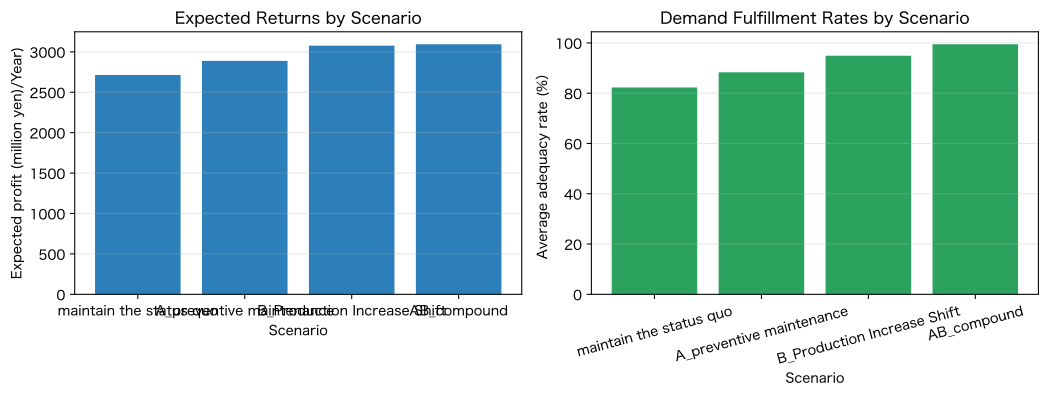
fig,axes=plt.subplots(1,2,figsize=(11,4.2)); axes[0].bar(summary["Scenario"],summary["expected benefit"]/1e6,color="#2c7fb8"); axes[0].set_title("Expected Returns by Scenario"); axes[0].set_xlabel("Scenario"); axes[0].set_ylabel("Expected profit (million yen)/Year)"); axes[0].grid(True,axis="y",alpha=.3); axes[1].bar(summary["Scenario"],summary["average adequacy rate"]*100,color="#2ca25f"); axes[1].set_title("Demand Fulfillment Rates by Scenario"); axes[1].set_xlabel("Scenario"); axes[1].set_ylabel("Average adequacy rate (%）"); axes[1].grid(True,axis="y",alpha=.3); plt.xticks(rotation=15); plt.tight_layout(); plt.show()

	Scenario	expected benefit	interest5%point	probability of loss	average adequacy rate	sufficiency rate95%less probability	Average ending inventory
0	maintain the status quo	¥2,713,302,647	¥2,602,642,065	0.0%	82.27%	100.0%	44
1	A_preventive maintenance	¥2,888,359,561	¥2,809,656,317	0.0%	88.30%	99.1%	129
2	B_Production Increase Shift	¥3,076,598,139	¥2,934,411,407	0.0%	94.89%	50.4%	2,828
3	AB_compound	¥3,093,538,649	¥2,717,132,026	0.0%	99.45%	1.4%	39,468

---

No.091: Understanding the Concept of Scenario Analysis

Meaning in Practice

Rather than a single project, we compare feasible future visions such as current status, conservation, increased production, and compound operations, all under the same premise.

Approach to Analysis and Modeling

Each scenario is defined as a set of capacity, stoppage, yield, fixed costs, and investment amount. Standardize random demand numbers to make differences in measures easier to see.

Check with Python

scenario_view=summary[["Scenario","expected benefit","interest5%point","average adequacy rate","Average ending inventory"]]; display(scenario_view.style.format({"expected benefit":"¥{:,.0f}","interest5%point":"¥{:,.0f}","average adequacy rate":"{:.2%}","Average ending inventory":"{:,.0f}"}))
fig,ax=plt.subplots();
for name,df in results.items(): ax.hist(df.profit/1e6,bins=35,alpha=.35,label=name)
ax.set_title("Annual profit distribution by scenario"); ax.set_xlabel("Annual profit (million yen)"); ax.set_ylabel("degree"); ax.grid(True,axis="y",alpha=.3); ax.legend(); plt.tight_layout(); plt.show()

	Scenario	expected benefit	interest5%point	average adequacy rate	Average ending inventory
0	maintain the status quo	¥2,713,302,647	¥2,602,642,065	82.27%	44
1	A_preventive maintenance	¥2,888,359,561	¥2,809,656,317	88.30%	129
2	B_Production Increase Shift	¥3,076,598,139	¥2,934,411,407	94.89%	2,828
3	AB_compound	¥3,093,538,649	¥2,717,132,026	99.45%	39,468

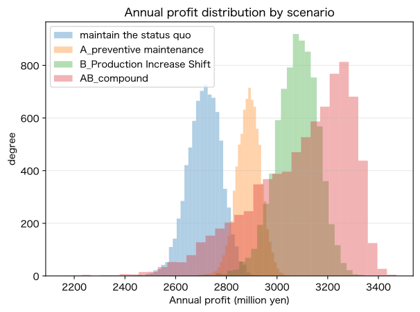
Reading the results

From the position and width of the distribution, you can compare not only average profits but also downside risk. Composite initiatives have characteristics that differ across multiple KPIs, such as having large supply capacity even at high costs.

---

No.092: Examining Key Parameters in Sensitivity Analysis

Meaning in Practice

Identify assumptions that influence conclusions and prioritize further investigations and contract negotiations.

Approach to Analysis and Modeling

Change the demand multiple, downtime multiple, and cost multiples of the base scenario one by one to measure changes in expected profit.

Check with Python

base_row=scenarios.iloc[0]; base_profit=results["maintain the status quo"].profit.mean(); sens=[]
for param,values in [("required magnification",[.9,1.1]),("Stop rate multiplier",[.7,1.3]),("cost ratio",[.95,1.05])]:
    for value in values:
        row=base_row.copy(); dm=cm=1.0
        if param=="required magnification": dm=value
        elif param=="Stop rate multiplier": row["downtime_scale"]=value
        else: cm=value
        sens.append({"Parameter":param,"Setting":value,"Expected profit spread":simulate(row,dm,cm).profit.mean()-base_profit})
sensitivity=pd.DataFrame(sens); display(sensitivity.style.format({"Setting":"{:.2f}","Expected profit spread":"¥{:+,.0f}"}))
fig,ax=plt.subplots(); piv=sensitivity.pivot(index="Parameter",columns="Setting",values="Expected profit spread"); piv.plot.barh(ax=ax); ax.set_title("Sensitivity Analysis Against Reference Profit"); ax.set_xlabel("Expected profit margin (yen)/Year)"); ax.set_ylabel("Parameter"); ax.grid(True,axis="x",alpha=.3); plt.tight_layout(); plt.show()

	Parameter	Setting	Expected profit spread
0	required magnification	0.90	¥-2,149,227
1	required magnification	1.10	¥+198,663
2	Stop rate multiplier	0.70	¥+93,041,622
3	Stop rate multiplier	1.30	¥-90,232,879
4	cost ratio	0.95	¥+206,783,556
5	cost ratio	1.05	¥-206,783,556

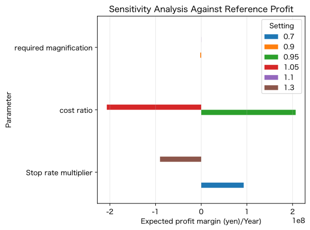
Reading the results

The higher the profit sensitivity, the higher the decision value, prioritizing demand research, cost contracts, and refinement of downtime records. Note that univariable sensitivity does not indicate interaction.

---

No.093: Set Based on the Status Quo Scenario

Meaning in Practice

The effectiveness of a measure is measured by the difference compared to ‘doing nothing.’ Maintaining the current status also involves risks of increased demand and aging.

Approach to Analysis and Modeling

Freeze capacity, stoppage, yield, and costs in reference cases, and calculate incremental KPIs for all measures based on the same criteria.

Check with Python

baseline=summary.query("`Scenario`=='maintain the status quo'").iloc[0]; incremental=summary.copy(); incremental["Incremental profit"]=incremental["expected benefit"]-baseline["expected benefit"]; incremental["Improvement in adequacy rate_pp"]=(incremental["average adequacy rate"]-baseline["average adequacy rate"])*100
display(incremental[["Scenario","Incremental profit","Improvement in adequacy rate_pp"]].style.format({"Incremental profit":"¥{:+,.0f}","Improvement in adequacy rate_pp":"{:+.2f}pt"}))
fig,ax=plt.subplots(); ax.bar(incremental["Scenario"],incremental["Incremental profit"]/1e6,color="#6baed6"); ax.axhline(0,color="black",linewidth=.8); ax.set_title("Incremental Profit on Maintaining the Status Quo"); ax.set_xlabel("Scenario"); ax.set_ylabel("Incremental profit (million yen)/Year)"); ax.grid(True,axis="y",alpha=.3); plt.tight_layout(); plt.show()

	Scenario	Incremental profit	Improvement in adequacy rate_pp
0	maintain the status quo	¥+0	+0.00pt
1	A_preventive maintenance	¥+175,056,914	+6.03pt
2	B_Production Increase Shift	¥+363,295,492	+12.62pt
3	AB_compound	¥+380,236,002	+17.19pt

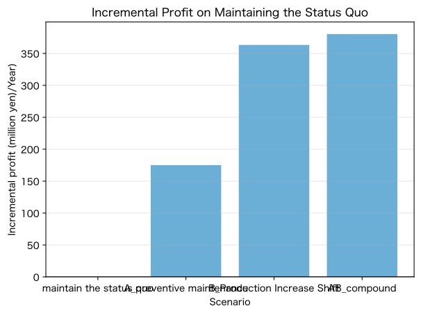
Reading the results

Incremental display clarifies what improvements or deteriorations the current measures are intended to make. Changes to the definition of comparison criteria affect all results, so version management is required.

---

No.094: Comparing Measures A and B

Meaning in Practice

Preventive maintenance A and increased production shift B are directly compared in terms of profit, delivery time, downside risk, and inventory.

Approach to Analysis and Modeling

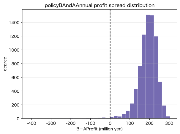
By calculating the difference $\Delta=Y_B-Y_A$ per trial using common random numbers, you can also evaluate the probability that B will surpass A.

Check with Python

a=results["A_preventive maintenance"]; bres=results["B_Production Increase Shift"]; diff=bres.profit-a.profit
ab=pd.DataFrame({"Comparison":["B-A"],"Average Profit Margin":[diff.mean()],"BHigh Profit Probability":[(diff>0).mean()],"Adequacy Rate Gap":[bres.service_rate.mean()-a.service_rate.mean()]})
display(ab.style.format({"Average Profit Margin":"¥{:,.0f}","BHigh Profit Probability":"{:.1%}","Adequacy Rate Gap":"{:+.2%}"}))
fig,ax=plt.subplots(); ax.hist(diff/1e6,bins=35,color="#756bb1",edgecolor="white"); ax.axvline(0,color="black",linestyle="--"); ax.set_title("policyBAndAAnnual profit spread distribution"); ax.set_xlabel("B－AProfit (million yen)"); ax.set_ylabel("degree"); ax.grid(True,axis="y",alpha=.3); plt.tight_layout(); plt.show()

	Comparison	Average Profit Margin	BHigh Profit Probability	Adequacy Rate Gap
0	B-A	¥188,238,578	98.8%	+6.59%

Reading the results

Even if B’s average profit is high, it doesn’t necessarily mean you win every trial. Combine profit spread probability and improvement in fulfillment rate, and select based on management risk tolerance.

---

No.095: Modeling Cost-Effectiveness

Meaning in Practice

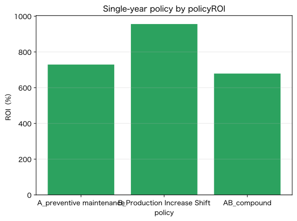
Divide incremental profit by the investment amount and compare ROI with the simple payback period.

Approach to Analysis and Modeling

$ROI=(E[\Pi_s]-E[\Pi_0])/I_s$. Collection period: $=I_s/(Incremental profit/12)$. Clearly indicate the duration of the benefit and the discount rate.

Check with Python

roi=incremental.merge(scenarios[["scenario","investment"]],left_on="Scenario",right_on="scenario"); roi=roi.query("investment>0").copy(); roi["ROI"]=roi["Incremental profit"]/roi["investment"]; roi["Number of months for collection"]=roi["investment"]/(roi["Incremental profit"]/12).replace(0,np.nan)
display(roi[["Scenario","Incremental profit","investment","ROI","Number of months for collection"]].style.format({"Incremental profit":"¥{:,.0f}","investment":"¥{:,.0f}","ROI":"{:.1%}","Number of months for collection":"{:.1f}month"}))
fig,ax=plt.subplots(); ax.bar(roi["Scenario"],roi["ROI"]*100,color="#2ca25f"); ax.axhline(0,color="black",linewidth=.8); ax.set_title("Single-year policy by policyROI"); ax.set_xlabel("policy"); ax.set_ylabel("ROI（%）"); ax.grid(True,axis="y",alpha=.3); plt.tight_layout(); plt.show()

	Scenario	Incremental profit	investment	ROI	Number of months for collection
1	A_preventive maintenance	¥175,056,914	¥24,000,000	729.4%	1.6month
2	B_Production Increase Shift	¥363,295,492	¥38,000,000	956.0%	1.3month
3	AB_compound	¥380,236,002	¥56,000,000	679.0%	1.8month

Reading the results

Even if ROI is high, proposals that do not meet supply targets cannot be adopted. For multi-year projects, NPV, residual value, and tax effects are also added.

---

No.096: Create a risk-taking decision sheet

Meaning in Practice

We present expected value, 5% points, loss probability, and service failure into a table, and simultaneously deliberate on returns and risks.

Approach to Analysis and Modeling

Add constraints to the decision table and clearly state hiring conditions such as an average fulfillment rate of 97% or higher and a loss probability of 5% or less.

Check with Python

decision=summary.copy(); decision["Service Conditions"]=decision["average adequacy rate"]>=.97; decision["Loss Conditions"]=decision["probability of loss"]<=.05; decision["Candidate for Employment"]=decision["Service Conditions"]&decision["Loss Conditions"]
display(decision.style.format({"expected benefit":"¥{:,.0f}","interest5%point":"¥{:,.0f}","probability of loss":"{:.1%}","average adequacy rate":"{:.2%}","sufficiency rate95%less probability":"{:.1%}","Average ending inventory":"{:,.0f}"}))

	Scenario	expected benefit	interest5%point	probability of loss	average adequacy rate	sufficiency rate95%less probability	Average ending inventory	Service Conditions	Loss Conditions	Candidate for Employment
0	maintain the status quo	¥2,713,302,647	¥2,602,642,065	0.0%	82.27%	100.0%	44	False	True	False
1	A_preventive maintenance	¥2,888,359,561	¥2,809,656,317	0.0%	88.30%	99.1%	129	False	True	False
2	B_Production Increase Shift	¥3,076,598,139	¥2,934,411,407	0.0%	94.89%	50.4%	2,828	False	True	False
3	AB_compound	¥3,093,538,649	¥2,717,132,026	0.0%	99.45%	1.4%	39,468	True	True	True

Reading the results

Putting hiring conditions in advance helps prevent choosing risky options based solely on expected returns. Condition values are determined based on customer contracts and financial capacity.

---

No.097: Visualizing and Explaining Model Results

Meaning in Practice

Expect profit and downside risk are communicated to management, while fullness rates and inventory are communicated to the field, all based on the same results.

Approach to Analysis and Modeling

Visualize the characteristics of your initiatives using a risk-return scatter plot and multiple standardized KPIs.

Check with Python

fig,axes=plt.subplots(1,2,figsize=(11,4.2))
axes[0].scatter(summary["interest5%point"]/1e6,summary["expected benefit"]/1e6,s=100)
for _,r in summary.iterrows(): axes[0].annotate(r["Scenario"],(r["interest5%point"]/1e6,r["expected benefit"]/1e6),xytext=(4,4),textcoords="offset points")
axes[0].set_title("Profit Risk and Return"); axes[0].set_xlabel("interest5%Points (million yen)"); axes[0].set_ylabel("Expected Profit (million yen)"); axes[0].grid(True,alpha=.3)
axes[1].scatter(summary["Average ending inventory"],summary["average adequacy rate"]*100,s=100,color="#de2d26")
for _,r in summary.iterrows(): axes[1].annotate(r["Scenario"],(r["Average ending inventory"],r["average adequacy rate"]*100),xytext=(4,4),textcoords="offset points")
axes[1].set_title("Inventory and Service Levels"); axes[1].set_xlabel("Average ending inventory (units)"); axes[1].set_ylabel("Average adequacy rate (%）"); axes[1].grid(True,alpha=.3); plt.tight_layout(); plt.show()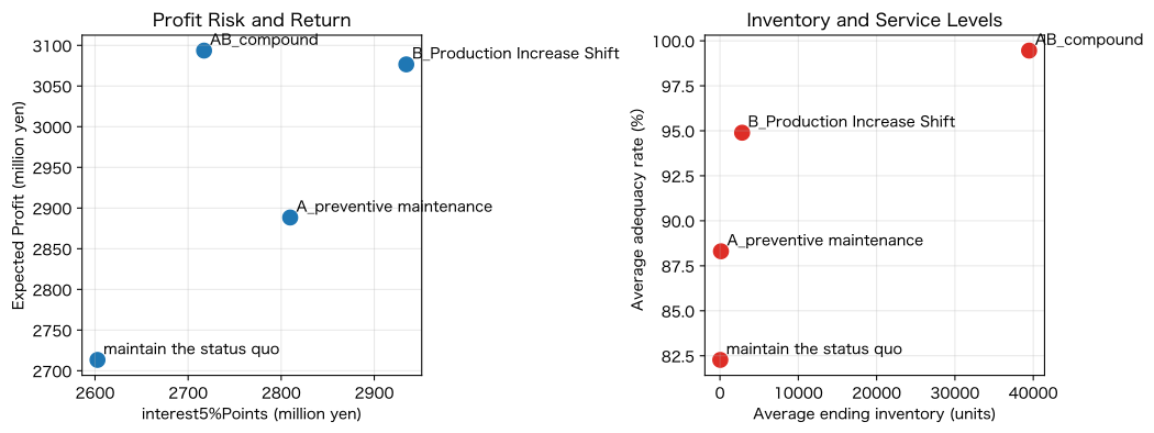

Reading the results

The top right shows the desired profit side, while the top left shows the desired inventory efficiency and service aspects. Choose axes based on your objectives and avoid showing only convenient indicators.

---

No.098: Organizing Model Limitations and Assumptions

Meaning in Practice

It clearly indicates the usable range of the model and what to do if it misses, preventing incorrect automatic judgments.

Approach to Analysis and Modeling

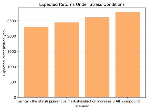
Assume a ledger of demand distribution, capacity, price, cost, independence, investment effect, and data period, and check results under stress conditions.

Check with Python

assumptions=pd.DataFrame({"premise":["Demand Growth","stop rate","yield rate","Sale Price","cost price","Ability Ceiling"],"standard":["month2.5%","past distribution","Average by Policy","5,200JPY","3,100JPY","Fixed by policy"],"If it comes off":["insufficient ability","Worsening delivery times","Increase in defects","profit reduction","profit reduction","Overtime and Outsourcing"]}); display(assumptions)
stress=[]
for name,row in scenarios.set_index("scenario").iterrows(): stress.append({"Scenario":name,"need+25%・Cost+10%interest":simulate(row,1.25,1.10).profit.mean()})
stress=pd.DataFrame(stress); display(stress.style.format({"need+25%・Cost+10%interest":"¥{:,.0f}"}))
fig,ax=plt.subplots(); ax.bar(stress["Scenario"],stress["need+25%・Cost+10%interest"]/1e6,color="#fdae6b"); ax.axhline(0,color="black"); ax.set_title("Expected Returns Under Stress Conditions"); ax.set_xlabel("Scenario"); ax.set_ylabel("Expected Profit (million yen)"); ax.grid(True,axis="y",alpha=.3); plt.tight_layout(); plt.show()

	premise	standard	If it comes off
0	Demand Growth	month2.5%	insufficient ability
1	stop rate	past distribution	Worsening delivery times
2	yield rate	Average by Policy	Increase in defects
3	Sale Price	5,200JPY	profit reduction
4	cost price	3,100JPY	profit reduction
5	Ability Ceiling	Fixed by policy	Overtime and Outsourcing

	Scenario	need+25%・Cost+10%interest
0	maintain the status quo	¥2,299,955,841
1	A_preventive maintenance	¥2,444,817,687
2	B_Production Increase Shift	¥2,612,757,372
3	AB_compound	¥2,785,372,850

Reading the results

We usually check whether the recommendations in the case are maintained under stress. If the assumption range is exceeded, a rule is needed to switch to recalculation and manual decision-making.

---

No.099: Organizing the Approach to a Mathematical Modeling Project

Meaning in Practice

We don’t just analyze but plan everything from problem definition, data, PoC, parallel operations, to implementation.

Approach to Analysis and Modeling

Decision-making, KPIs, responsible persons, deliverables, and evaluation criteria are set at each stage, and model accuracy and operational effectiveness are evaluated separately.

Check with Python

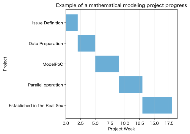
project=pd.DataFrame({"Project":["Issue Definition","Data Preparation","ModelPoC","Parallel operation","Established in the Real Sex"],"Start week":[0,2,5,9,13],"Period Week":[2,3,4,4,5],"deliverable":["Decision-making/KPI","Data dictionary","Comparative Model","Operational Evaluation","Monitoring and Update Procedures"]}); display(project)
fig,ax=plt.subplots();
for i,r in project.iterrows(): ax.barh(r["Project"],r["Period Week"],left=r["Start week"],color="#6baed6")
ax.set_title("Example of a mathematical modeling project progress"); ax.set_xlabel("Project Week"); ax.set_ylabel("Project"); ax.grid(True,axis="x",alpha=.3); ax.invert_yaxis(); plt.tight_layout(); plt.show()

	Project	Start week	Period Week	deliverable
0	Issue Definition	0	2	Decision-making/KPI
1	Data Preparation	2	3	Data dictionary
2	ModelPoC	5	4	Comparative Model
3	Parallel operation	9	4	Operational Evaluation
4	Established in the Real Sex	13	5	Monitoring and Update Procedures

Reading the results

If you skip problem definition and data organization, even if the model is highly accurate, it will not be used. We review the differences from current judgments through parallel operation.

---

No.100: Designing decision support models from business challenges

Meaning in Practice

Finally, it integrates issues, inputs, models, outputs, decision criteria, and operations into a single decision design.

Approach to Analysis and Modeling

The recommended rule is to maximize expected profit among proposals that meet the service and loss conditions. If none applicable, the relaxation of restrictions will be returned to management.

Check with Python

candidates=decision.query("`Candidate for Employment`"); recommended=(candidates.loc[candidates["expected benefit"].idxmax()] if len(candidates) else decision.loc[decision["interest5%point"].idxmax()])
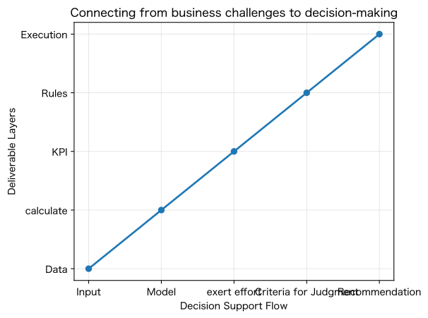
design=pd.DataFrame({"element":["Business Challenges","Input","Model","exert effort","Criteria for Judgment","Recommendation","Utilization"],"Contents":["Capacity and Conservation Investment to Increase Demand","Demand, Stoppages, Yield, Price, Cost, Expenses","12Monte Carlo Moon","Profit Distribution, Fulfillment Ratio, Inventory,ROI","sufficiency rate≥97%, loss probability≤5%Maximum expected profit",recommended["Scenario"],"Monthly updates, quarterly re-evaluations, and recalculations when assumptions deviate"]}); display(design)
fig,ax=plt.subplots(); order=["Input","Model","exert effort","Criteria for Judgment","Recommendation"]; ax.plot(range(len(order)),range(len(order)),marker="o",linewidth=2); ax.set_xticks(range(len(order)),order); ax.set_yticks(range(len(order)),["Data","calculate","KPI","Rules","Execution"]); ax.set_title("Connecting from business challenges to decision-making"); ax.set_xlabel("Decision Support Flow"); ax.set_ylabel("Deliverable Layers"); ax.grid(True,alpha=.3); plt.tight_layout(); plt.show(); print(f"Recommended Scenario: {recommended['Scenario']} / expected benefit ¥{recommended['expected benefit']:,.0f} / sufficiency rate {recommended['average adequacy rate']:.2%}")

	element	Contents
0	Business Challenges	Capacity and Conservation Investment to Increase Demand
1	Input	Demand, Stoppages, Yield, Price, Cost, Expenses
2	Model	12Monte Carlo Moon
3	exert effort	Profit Distribution, Fulfillment Ratio, Inventory,ROI
4	Criteria for Judgment	sufficiency rate≥97%, loss probability≤5%Maximum expected profit
5	Recommendation	AB_compound
6	Utilization	Monthly updates, quarterly re-evaluations, and recalculations when assumptions deviate

Recommended scenario: AB_ compound / Expected profit ¥3,093,538,649 / Fulfillment rate 99.45%

Reading the results

This is a decision support model that includes not only recommendations, but also hiring conditions, input, update frequency, and recalculation conditions. Final approvals are made based on on-site knowledge and management responsibility.

---

Practical Implications Seen Through Target Exercise

Scenarios are compared using the same criteria and clearly indicate maintaining the status quo. Sensitivity analysis identifies key assumptions and simultaneously presents ROI and risk. Visualization aligns with the recipient’s judgment, concealing its limits and scope of application. Model building does not end with PoC; it must be designed for parallel operation, monitoring, updates, and re-approval.

What is necessary for practical implementation

1. Decide on decision-making and approval conditions first

Agree on profits, services, loss tolerance, and investment limits.

2. Unify scenario assumptions and manage the version

Sources for demand, price, capacity, cost, and effectiveness of measures are retained.

3. Compare common random numbers with backtesting

We separate policy differences from random numbers and check reproducibility over past periods.

4. Define Model Limits and Manual Judgment

Supply suspensions, large orders, and major quality incidents are reassigned to exceptional operations.

5. Measure operational effectiveness through parallel operation

It measures not only accuracy but also out-of-stock items, inventory, overtime, and decision-making time.

6. Decide on renewal, monitoring, and responsibility

Monthly input, quarterly re-estimation, and assumption deviation alerts are operated.

Conclusion

No.091–100 integrated scenarios, sensitivity, baseline cases, measure comparisons, ROI, risk, visualization, limitations, and project progress, designing decision support models based on business challenges. The completion of a mathematical model is not the result of calculations, but a state where the organization can share assumptions and trade-offs and make continuous judgments.

Consultations for Corporations

At Surikoubo, we support scenario analysis, Monte Carlo simulations, decision support models for investment, production, inventory, and maintenance, and support from PoC to operational implementation.

📩 Contact Us: surikobo.co.jp/contact Please feel free to consult us first.