Predicting the “next state” of equipment, customers, and inventory

State Transition Models Learned at Industrial Equipment Manufacturers No.071–No.080

This article focuses on the after-sales service of industrial equipment manufacturers, representing the health of equipment, customer operation, hibernation, and churn, spare parts inventory, and sales funnel as condition variables. Check transition probabilities, Markov models, failures and maintenance, and future states before and after measures in Python.

[!NOTE] This material is a notebook previously used by Surikoubo (or personally by the representative, Kazuyama), and has been reconstructed, edited, and published with the company’s permission. All data listed is fictional and has no relation whatsoever to real companies, factories, or figures.

Introduction: Practical Challenges in Manufacturing Covered in This Article

Equipment manufacturers monitor the weekly health status of 60 delivered machines. Preventive maintenance on abnormal equipment reduces failures but incurs maintenance costs and downtime. Additionally, customers purchasing replacement parts move through cycles of operation, dormancy, and departure, and sales deals progress through multiple stages.

We model not only the number of cases per month but also “where to move from the current state” to evaluate future structure and policy effectiveness.

Common situations on site

• Only the number of normal units is counted, without checking the speed at which the alert moves to abnormal.
• Sensor thresholds and conservation actions are not linked.
• It does not compare the recovery probability of post-breakdown repairs with preventive maintenance.
• Look only at the final result of customer churn and avoid chasing the signs of dormancy.
• No one knows how inventory shortages and surpluses will remain the next week.
• Each stage of the sales funnel is managed as an independent KPI

Why is this issue so difficult to judge?

The state carries over between time points. The number of abnormal vehicles depends not only on the number of newly deteriorated vehicles but also on the number of vehicles that have recovered or malfunctioned from the previous week’s abnormalities.

In the state transition model, the set of states is defined exclusively and each row of transition probability is 1. The Markov model is a simplification, meaning ‘the following state depends on the current state,’ and if elapsed time or history is important, it breaks down the state.

Overview of Exercise covered this time

No.	Theme	Practical Judgment
071	State variable	What to hold as a state
072	Customer Status	How to define operating, hibernation, and defection
073	migration probability	How to create a probability matrix from achievements
074	Markov Model	How to predict state composition several weeks ahead
075	customer defection	How much dormancy measures reduce defections.
076	Facility Condition	Changing sensor values to normal, caution, or abnormal
077	Breakdowns and Maintenance	How do the chances of recovery and breakdown differ depending on whether maintenance is maintained?
078	Stock Status	How to measure the persistence of excess, adequacy, and deficiency
079	Purchase funnel	How to predict future numbers at the negotiation stage
080	Measure Evaluation	How to compare the cost of preventive maintenance and failure reduction

Preparing the Python environment

No external data is used. Fix the random number seed and generate the state sequence and transition matrix using NumPy, pandas, and matplotlib.

%matplotlib inline
%config InlineBackend.figure_format = 'svg'
import platform,sys
import matplotlib, matplotlib.pyplot as plt
from matplotlib import font_manager
import numpy as np, pandas as pd
from IPython.display import display
SEED=42; rng=np.random.default_rng(SEED)
fonts={f.name for f in font_manager.fontManager.ttflist}; plot_font=next((f for f in ["Hiragino Sans","Yu Gothic","Noto Sans CJK JP"] if f in fonts),"sans-serif")
plt.rcParams["font.family"]=plot_font; plt.rcParams["axes.unicode_minus"]=False
print(f"Python {sys.version.split()[0]} / NumPy {np.__version__} / pandas {pd.__version__} / matplotlib {matplotlib.__version__}")
print(f"font {plot_font} / seed {SEED} / {platform.platform()}")

Python 3.13.1 / NumPy 2.5.1 / pandas 3.0.3 / matplotlib 3.11.0
font Hiragino Sans / seed 42 / macOS-26.3-arm64-arm-64bit-Mach-O

Creation of Fictional Data

Tracks 60 units for 52 weeks, transitioning between normal, caution, abnormal, and malfunction. In some cases of abnormalities, preventive maintenance is implemented to improve transition probability. At the same time, it generates 400 customer companies and 18 months of operating, dormant, or defection status.

eq_states=["Normal","Caution","Abnormal","Failure"]
P_eq=np.array([[.90,.08,.015,.005],[.18,.65,.13,.04],[.05,.20,.55,.20],[.65,.05,0,.30]])
P_maint=np.array([.75,.20,.04,.01])
eq_rows=[]
for machine in range(60):
    state="Normal"
    for week in range(52):
        action=(state=="Abnormal" and rng.random()<.55)
        probs=P_maint if action else P_eq[eq_states.index(state)]
        nxt=rng.choice(eq_states,p=probs)
        vib_mean={"Normal":1.2,"Caution":2.1,"Abnormal":3.2,"Failure":4.5}[state]
        eq_rows.append({"machine":machine+1,"week":week,"state":state,"next_state":nxt,"maintenance":action,"vibration":max(0,rng.normal(vib_mean,.22))})
        state=nxt
equipment=pd.DataFrame(eq_rows)

cust_states=["Active","Dormant","Churned"]
P_cust=np.array([[.87,.10,.03],[.20,.63,.17],[0,0,1]])
cust_rows=[]
for customer in range(400):
    state="Active"
    for month in range(18):
        nxt=rng.choice(cust_states,p=P_cust[cust_states.index(state)])
        cust_rows.append({"customer":customer+1,"month":month,"state":state,"next_state":nxt})
        state=nxt
customers=pd.DataFrame(cust_rows)
print(f"equipment migration: {len(equipment):,}records / customer migration: {len(customers):,}records")
display(equipment.head(8).style.format({"vibration":"{:.2f}"}))

Equipment migration: 3,120 items / Customer migration: 7,200 items

	machine	week	state	next_state	maintenance	vibration
0	1	0	Normal	Normal	False	0.97
1	1	1	Normal	Normal	False	1.41
2	1	2	Normal	Normal	False	0.91
3	1	3	Normal	Normal	False	1.13
4	1	4	Normal	Normal	False	1.01
5	1	5	Normal	Normal	False	1.37
6	1	6	Normal	Normal	False	1.45
7	1	7	Normal	Normal	False	1.01

eq_share=pd.crosstab(equipment["week"],equipment["state"],normalize="index").reindex(columns=eq_states,fill_value=0)
cust_share=pd.crosstab(customers["month"],customers["state"],normalize="index").reindex(columns=cust_states,fill_value=0)
fig,axes=plt.subplots(1,2,figsize=(11,4.2))
eq_share.plot.area(ax=axes[0],stacked=True); axes[0].set_title("Weekly Trends in Equipment Condition Configuration"); axes[0].set_xlabel("week"); axes[0].set_ylabel("Composition ratio"); axes[0].grid(True,alpha=.3)
cust_share.plot.area(ax=axes[1],stacked=True); axes[1].set_title("Monthly Trends in Customer Status Composition"); axes[1].set_xlabel("month"); axes[1].set_ylabel("Composition ratio"); axes[1].grid(True,alpha=.3)
plt.tight_layout(); plt.show()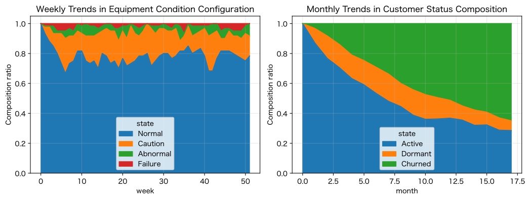

---

No.071: Understanding the Concept of State Variables

Meaning in Practice

State variables are information carried over to determine the next point in time. For equipment, it falls under health status; for inventory, it falls under the surplus and shortage category.

Approach to Analysis and Modeling

$S_t\in\{normal,Note,abnormal,malfunction\}$ is defined as this, and each point in time is always given one state. State definitions should be mutually exclusive and comprehensive.

Check with Python

sample=equipment.query("machine==1")
state_num={"Normal":0,"Caution":1,"Abnormal":2,"Failure":3}
fig,ax=plt.subplots(); ax.step(sample["week"],sample["state"].map(state_num),where="post",color="#2c7fb8"); ax.set_yticks(range(4),["normal","Note","abnormal","malfunction"]); ax.set_title("Equipment1Unit 1 State Variables"); ax.set_xlabel("week"); ax.set_ylabel("Facility Condition"); ax.grid(True,alpha=.3); plt.tight_layout(); plt.show()
print(sample["state"].value_counts().to_string())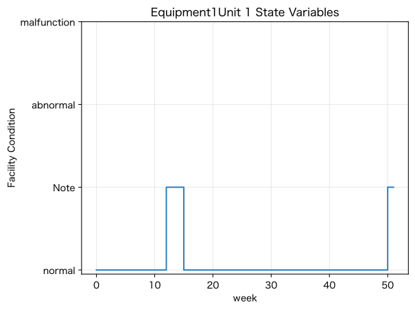

state
Normal     47
Caution     5

Reading the results

With the state series, you can track sustained attention, deterioration of abnormalities, and recovery on the same axis. Adding the duration of stay to the status allows you to prioritize long-term abnormalities.

---

No.072: Modeling Customer Conditions

Meaning in Practice

Breaking down replacement parts customers into active, dormant, and churn helps manage early signs of sales decline and reactivation.

Approach to Analysis and Modeling

Operation is defined by observable rules, such as a recent purchase for a recent purchase, dormancy for a certain period without purchase, and defection as contract termination.

Check with Python

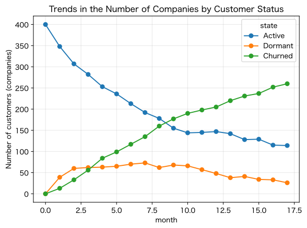
customer_counts=pd.crosstab(customers["month"],customers["state"]).reindex(columns=cust_states,fill_value=0)
display(customer_counts.tail(8))
fig,ax=plt.subplots(); customer_counts.plot(ax=ax,marker="o"); ax.set_title("Trends in the Number of Companies by Customer Status"); ax.set_xlabel("month"); ax.set_ylabel("Number of customers (companies)"); ax.grid(True,alpha=.3); plt.tight_layout(); plt.show()

state	Active	Dormant	Churned
month
10	144	66	190
11	145	57	198
12	147	48	205
13	142	38	220
14	128	41	231
15	129	34	237
16	115	33	252
17	114	26	260

Reading the results

Churn accumulates, and the number of active customers decreases. The number of dormant customers serves as a leading indicator of future churn and is subject to repurchase strategies.

---

No.073: Modeling State Transition Probability

Meaning in Practice

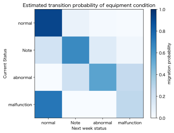
The transition probability represents the percentage of the following state for each current state, allowing comparison of the speed of deterioration and recovery.

Approach to Analysis and Modeling

$p_{ij}=P(S_{t+1}=j\mid S_t=i)$。 Normalize the cross table of entries in the row direction and check whether each line sum is 1.

Check with Python

no_action=equipment.query("not maintenance")
P_hat=pd.crosstab(no_action["state"],no_action["next_state"],normalize="index").reindex(index=eq_states,columns=eq_states,fill_value=0)
display(P_hat.style.format("{:.1%}")); print("Peace:",P_hat.sum(axis=1).round(6).to_dict())
fig,ax=plt.subplots(); im=ax.imshow(P_hat,cmap="Blues",vmin=0,vmax=1); ax.set_xticks(range(4),["normal","Note","abnormal","malfunction"]); ax.set_yticks(range(4),["normal","Note","abnormal","malfunction"]); ax.set_title("Estimated transition probability of equipment condition"); ax.set_xlabel("Next week status"); ax.set_ylabel("Current Status"); ax.grid(False); plt.colorbar(im,ax=ax,label="migration probability"); plt.tight_layout(); plt.show()

next_state	Normal	Caution	Abnormal	Failure
state
Normal	91.4%	6.4%	1.4%	0.7%
Caution	18.5%	65.6%	12.4%	3.5%
Abnormal	0.0%	20.0%	55.0%	25.0%
Failure	72.7%	0.0%	0.0%	27.3%

Sum of rows: {'Normal': 1.0, 'Caution': 1.0, 'Abnormal': 1.0, 'Failure': 1.0}

Reading the results

The diagonal component represents continuation, the right side represents deterioration, and the left side represents recovery. Since the estimation error is large in the state with a small number of cases, confidence intervals and stratification are considered.

---

No.074: Understanding the Markov Model Concept

Meaning in Practice

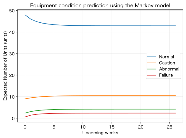
Based on the current state configuration and transition matrix, you can predict the number of normal, cautionary, abnormal, and faulty units several weeks ahead.

Approach to Analysis and Modeling

The state distribution vector $\pi_t$ is updated at $\pi_{t+k}=\pi_tP^k$. Let’s assume Markov’s principle, which determines the next step based solely on the current state.

Check with Python

pi0=np.array([.80,.15,.04,.01]); forecasts=[]
for k in range(27): forecasts.append({"week":k,**dict(zip(eq_states,pi0@np.linalg.matrix_power(P_hat.to_numpy(),k)))})
markov=pd.DataFrame(forecasts)
display(markov.iloc[::5].style.format({s:"{:.1%}" for s in eq_states}))
fig,ax=plt.subplots();
for s in eq_states: ax.plot(markov["week"],markov[s]*60,label=s)
ax.set_title("Equipment condition prediction using the Markov model"); ax.set_xlabel("Upcoming weeks"); ax.set_ylabel("Expected Number of Units (units)"); ax.grid(True,alpha=.3); ax.legend(); plt.tight_layout(); plt.show()

	week	Normal	Caution	Abnormal	Failure
0	0	80.0%	15.0%	4.0%	1.0%
5	5	72.4%	17.1%	6.7%	3.8%
10	10	71.6%	17.4%	7.0%	4.0%
15	15	71.5%	17.5%	7.0%	4.0%
20	20	71.5%	17.5%	7.0%	4.0%
25	25	71.5%	17.5%	7.0%	4.0%

Reading the results

Converging from the initial configuration to the long-term configuration. If the maintenance history or status retention period applies to the next state, the status will be extended to ‘Caution Week 1’ or similar.

---

No.075: Expressing Customer Churn as a State Transition

Meaning in Practice

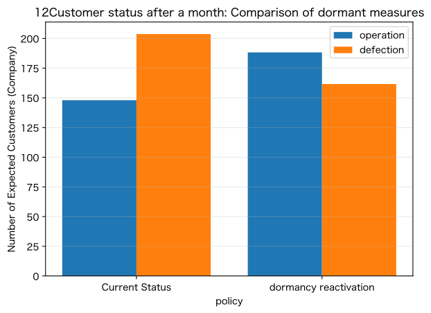
By implementing measures for dormant customers, you can estimate the future number of customers if you increase the probability of reactivation and reduce the probability of churn.

Approach to Analysis and Modeling

The reference matrix and the policy matrix are sprung by 12 to compare the state distribution of the initial 400 customers.

Check with Python

P_base=P_cust.copy(); P_action=P_cust.copy(); P_action[1]=[.32,.58,.10]
initial=np.array([1.,0,0]); rows=[]
for name,P in [("Current Status",P_base),("dormancy reactivation",P_action)]:
    dist=initial@np.linalg.matrix_power(P,12); rows.append({"policy":name,**{s:dist[i]*400 for i,s in enumerate(cust_states)}})
churn_eval=pd.DataFrame(rows); display(churn_eval.style.format({s:"{:.1f}society" for s in cust_states}))
fig,ax=plt.subplots(); x=np.arange(2); ax.bar(x-.2,churn_eval["Active"],.4,label="operation"); ax.bar(x+.2,churn_eval["Churned"],.4,label="defection"); ax.set_xticks(x,churn_eval["policy"]); ax.set_title("12Customer status after a month: Comparison of dormant measures"); ax.set_xlabel("policy"); ax.set_ylabel("Number of Expected Customers (Company)"); ax.grid(True,axis="y",alpha=.3); ax.legend(); plt.tight_layout(); plt.show()

	policy	Active	Dormant	Churned
0	Current Status	148.0society	48.3society	203.7society
1	dormancy reactivation	188.2society	50.1society	161.6society

Reading the results

Increasing the return rate from dormancy to operation increases the number of active customers after 12 months and reduces churn. We will make decisions based on both the initiative cost and the additional gross profit.

---

No.076: Expressing Equipment Status as Normal, Caution, or Abnormal

Meaning in Practice

By converting continuous sensor values into actionable states, you can unify the rules for monitoring, re-measurement, and inspection.

Approach to Analysis and Modeling

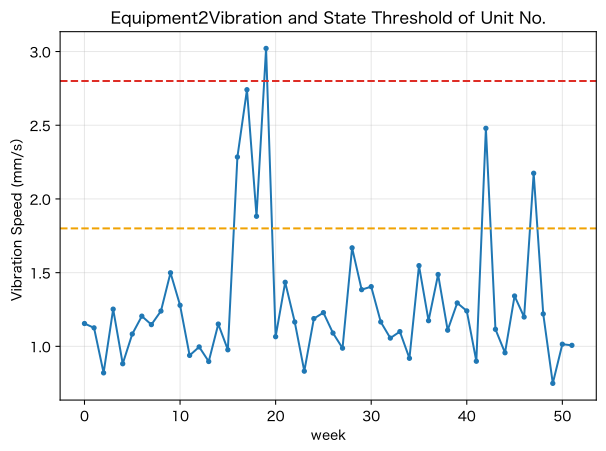
Vibration values are classified as normal $v<1.8$, caution $1.8\le v<2.8$, or abnormal $v\ge2.8$. Thresholds are set to balance missed and false alarms.

Check with Python

equipment["sensor_state"]=pd.cut(equipment["vibration"],[-np.inf,1.8,2.8,np.inf],labels=["normal","Note","abnormal"],right=False)
sensor_counts=pd.crosstab(equipment["state"],equipment["sensor_state"]); display(sensor_counts)
sample=equipment.query("machine==2")
fig,ax=plt.subplots(); ax.plot(sample["week"],sample["vibration"],marker="o",markersize=3); ax.axhline(1.8,color="#f0a202",linestyle="--"); ax.axhline(2.8,color="#de2d26",linestyle="--"); ax.set_title("Equipment2Vibration and State Threshold of Unit No."); ax.set_xlabel("week"); ax.set_ylabel("Vibration Speed (mm/s）"); ax.grid(True,alpha=.3); plt.tight_layout(); plt.show()

sensor_state	normal	Note	abnormal
state
Abnormal	0	4	123
Caution	57	434	0
Failure	0	0	66
Normal	2425	11	0

Reading the results

You can extract anomaly candidates based on thresholds. Compare sensor status with actual faults and inspection results, and update by equipment type.

---

No.077: Expressing Failure and Maintenance as State Transitions

Meaning in Practice

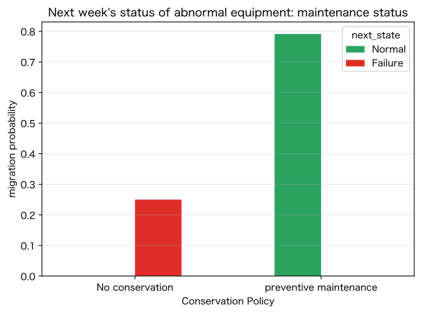
You can compare the recovery and failure probabilities when maintenance is done with and without abnormal equipment, and explain the effectiveness of preventive maintenance.

Approach to Analysis and Modeling

Starting from the abnormal state, the conditional probability of the next week’s state is estimated based on whether or not it is maintained. Because of selection bias, experimental design is necessary to determine causal effects.

Check with Python

abn=equipment.query("state=='Abnormal'"); maint_transition=pd.crosstab(abn["maintenance"],abn["next_state"],normalize="index").reindex(index=[False,True],columns=eq_states,fill_value=0); maint_transition.index=["No conservation","preventive maintenance"]
display(maint_transition.style.format("{:.1%}"))
fig,ax=plt.subplots(); maint_transition[["Normal","Failure"]].plot.bar(ax=ax,color=["#2ca25f","#de2d26"]); ax.set_title("Next week's status of abnormal equipment: maintenance status"); ax.set_xlabel("Conservation Policy"); ax.set_ylabel("migration probability"); ax.grid(True,axis="y",alpha=.3); plt.xticks(rotation=0); plt.tight_layout(); plt.show()

next_state	Normal	Caution	Abnormal	Failure
No conservation	0.0%	20.0%	55.0%	25.0%
preventive maintenance	79.1%	19.4%	1.5%	0.0%

Reading the results

Preventive maintenance increases the chances of recovery to normal and reduces the transition to failure. Maintenance costs, planned shutdowns, and failure losses are integrated in No.080.

---

No.078: Expressing inventory status as excess, adequacy, or shortage

Meaning in Practice

By converting inventory quantities into states, you can manage the probability of surplus or shortage continuing into the following week and the recovery to appropriate inventory.

Approach to Analysis and Modeling

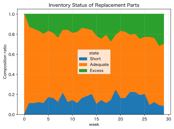
Set inventory cover days to less than 5 days, appropriate 5 to 15 days, and excess over 15 days, generating weekly transitions.

Check with Python

inv_states=["Short","Adequate","Excess"]; P_inv=np.array([[.45,.50,.05],[.12,.76,.12],[.04,.42,.54]])
inv_rows=[]
for item in range(100):
    s="Adequate"
    for week in range(30):
        nxt=rng.choice(inv_states,p=P_inv[inv_states.index(s)]); inv_rows.append((item,week,s,nxt)); s=nxt
inventory=pd.DataFrame(inv_rows,columns=["item","week","state","next_state"])
P_inv_hat=pd.crosstab(inventory["state"],inventory["next_state"],normalize="index").reindex(index=inv_states,columns=inv_states); display(P_inv_hat.style.format("{:.1%}"))
share=pd.crosstab(inventory["week"],inventory["state"],normalize="index").reindex(columns=inv_states,fill_value=0)
fig,ax=plt.subplots(); share.plot.area(ax=ax); ax.set_title("Inventory Status of Replacement Parts"); ax.set_xlabel("week"); ax.set_ylabel("Composition ratio"); ax.grid(True,alpha=.3); plt.tight_layout(); plt.show()

next_state	Short	Adequate	Excess
state
Short	40.4%	54.4%	5.1%
Adequate	12.1%	74.4%	13.5%
Excess	4.2%	40.4%	55.3%

Reading the results

Items with a high probability of continuous shortage or excess are not temporary exceptions but subject to review of order points and lot settings.

---

No.079: Expressing the Purchase Funnel as a State Transition

Meaning in Practice

By considering recognition, inquiries, proposals, orders, and lost orders, you can predict future order volumes and bottlenecks.

Approach to Analysis and Modeling

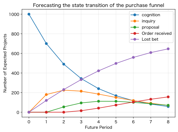
Orders are absorbed and lost, and the funnel transition matrix is multiplied. It can also express returns or stagnation.

Check with Python

f_states=["cognition","inquiry","proposal","Order received","Lost bet"]
P_f=np.array([[.70,.18,0,0,.12],[0,.55,.30,0,.15],[0,.05,.50,.28,.17],[0,0,0,1,0],[0,0,0,0,1]])
initial=np.array([1000,0,0,0,0.]); funnel=[]
for k in range(9): funnel.append({"Period":k,**dict(zip(f_states,initial@np.linalg.matrix_power(P_f,k)))})
funnel=pd.DataFrame(funnel); display(funnel.style.format({s:"{:.1f}" for s in f_states}))
fig,ax=plt.subplots();
for s in f_states: ax.plot(funnel["Period"],funnel[s],marker="o",label=s)
ax.set_title("Forecasting the state transition of the purchase funnel"); ax.set_xlabel("Future Period"); ax.set_ylabel("Number of Expected Projects"); ax.grid(True,alpha=.3); ax.legend(); plt.tight_layout(); plt.show()

	Period	cognition	inquiry	proposal	Order received	Lost bet
0	0	1000.0	0.0	0.0	0.0	0.0
1	1	700.0	180.0	0.0	0.0	120.0
2	2	490.0	225.0	54.0	0.0	231.0
3	3	343.0	214.7	94.5	15.1	332.7
4	4	240.1	184.5	111.6	41.6	422.2
5	5	168.1	150.3	111.2	72.8	497.6
6	6	117.6	118.5	100.7	104.0	559.2
7	7	82.4	91.4	85.9	132.2	608.2
8	8	57.6	69.4	70.4	156.2	646.4

Reading the results

As the period passes, orders are absorbed into both orders and losses. You can estimate how improvements in transitioning from proposal to order will affect final orders.

---

No.080: Using State Transition Models for Policy Evaluation

Meaning in Practice

When the transition probability is changed during preventive maintenance, future failures, downtime losses, and maintenance costs are compared.

Approach to Analysis and Modeling

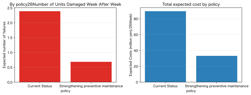
The current status matrix and the policy matrix that is easier to recover from warnings and anomalies will be updated up to 26 weeks ahead. The cost is estimated as 1,500,000 yen per week × a broken bike and maintenance fees.

Check with Python

P_policy=P_hat.to_numpy().copy(); P_policy[1]=[.30,.62,.07,.01]; P_policy[2]=[.55,.30,.12,.03]
pi=np.array([.80,.15,.04,.01]); rows=[]
for name,P,maint_cost in [("Current Status",P_hat.to_numpy(),0),("Strengthening preventive maintenance",P_policy,6_500_000)]:
    dist=pi.copy(); failure_weeks=0
    for _ in range(26): dist=dist@P; failure_weeks+=dist[3]*60
    loss=failure_weeks*1_500_000+maint_cost
    rows.append({"policy":name,"26Normal channel after the week":dist[0]*60,"26Breakdown platform after the week":dist[3]*60,"Cumulative Breakdown Weeks":failure_weeks,"Security fee":maint_cost,"Total expected cost":loss})
policy=pd.DataFrame(rows); display(policy.style.format({"26Normal channel after the week":"{:.1f}","26Breakdown platform after the week":"{:.1f}","Cumulative Breakdown Weeks":"{:.1f}","Security fee":"¥{:,.0f}","Total expected cost":"¥{:,.0f}"}))
fig,axes=plt.subplots(1,2,figsize=(11,4.2)); axes[0].bar(policy["policy"],policy["26Breakdown platform after the week"],color="#de2d26"); axes[0].set_title("By policy26Number of Units Damaged Week After Week"); axes[0].set_xlabel("policy"); axes[0].set_ylabel("Expected number of failures"); axes[0].grid(True,axis="y",alpha=.3); axes[1].bar(policy["policy"],policy["Total expected cost"]/1e6,color="#2c7fb8"); axes[1].set_title("Total expected cost by policy"); axes[1].set_xlabel("policy"); axes[1].set_ylabel("Expected Costs (million yen)/26Week)"); axes[1].grid(True,axis="y",alpha=.3); plt.tight_layout(); plt.show()
print(f"Expected cost savings: ¥{policy.loc[0,'Total expected cost']-policy.loc[1,'Total expected cost']:,.0f}")

	policy	26Normal channel after the week	26Breakdown platform after the week	Cumulative Breakdown Weeks	Security fee	Total expected cost
0	Current Status	42.9	2.4	59.6	¥0	¥89,474,389
1	Strengthening preventive maintenance	48.4	0.7	17.8	¥6,500,000	¥33,155,592

Expected cost reduction: ¥56,318,797

Reading the results

Enhanced preventive maintenance increases maintenance costs but may reduce downtime weeks and total expected costs. Sensitivity analysis is performed on the estimation error of transition probabilities, and small-scale verification is conducted on-site.

---

Practical Implications Seen Through Target Exercise

State variables are information carried over between time points. The transition matrix simultaneously represents deterioration, recovery, and continuation, and future configurations can be predicted using matrix powers. Equipment, customers, inventory, and sales can be handled with the same concept, but it is necessary to check state definitions, absorption status, historical dependence, and policy selection bias.

What is necessary for practical implementation

1. Standardize state definitions and determination times

Define observable rules for normal, cautionary, abnormal, operational, and dormant status.

2. Maintain history with individual ID

Connect data across equipment, customers, items, and projects at different points.

3. Check the number of transitions and uncertainty

Do not overestimate the probability of minority states; set confidence intervals and update frequency.

4. Incorporate history dependencies into state

Abnormal continuation weeks, elapsed months for customers, and days after maintenance are added to the status as needed.

5. Causally verify the effectiveness of the measures

Considering biases in conservation target selection, verification is conducted through comparison groups and phased introductions.

6. Connect to Costs and Constraints

We assess the impact amount of failures, turnovers, out-of-stock, or lost orders together with the cost of measures.

Conclusion

No.071–080 represent equipment, customers, inventory, and purchasing funnels as state transitions, connecting transition probabilities, Markov predictions, and evaluations of preservation and divergence measures. It is important not only to see the current number of cases but also to see how quickly the condition worsens or recovers.

Consultations for Corporations

At Mathematical Laboratory, we support transitional analysis of equipment status, customer churn, inventory status, sales funnel transitions, preventive maintenance, policy evaluation, and operational design of condition KPIs.

📩 Contact Us: surikobo.co.jp/contact Please feel free to consult us first.