不確実性を織り込む営業・技術支援計画：ベイズ回帰で受注額・受注確率・問い合わせ件数を読む

概要

製造業の営業・技術支援では、限られた実績から「来月の受注額」「案件ごとの受注確率」「問い合わせ件数」を見積もる必要があります。本稿では、架空の産業機器メーカーを題材に、ベイズ線形回帰・ベイズロジスティック回帰・ベイズポアソン回帰を一つの意思決定プロセスとして実装します。点予測だけでなく、係数や予測の不確実性まで可視化し、予算、人員、案件優先順位へつなげます。

[!NOTE] 本資料は、数理工房 (もしくは代表である和山個人) が過去に企業研修において使用した notebook を企業様の許可を得て再構成・編集のうえ公開しています。
掲載データはすべて架空のものであり、実在する企業・工場・数値とは一切関係ありません。

はじめに：この記事で扱う製造業の実務課題

産業機器は案件単価が高く、商談期間も長いため、平均値だけの計画は外れたときの影響が大きくなります。ここでは、月次の販促・営業活動から受注額を予測し、見積案件の受注確率でフォロー順位を決め、製品稼働台数から技術問い合わせ対応要員を計画します。

現場でよくある状況

• 実績が数十件しかなく、通常の回帰係数が大きく動く
• 営業施策と受注額の関係を知りたいが、季節性やばらつきも大きい
• 案件を「受注／失注」、問い合わせを「件数」として適切に扱いたい
• 経営会議では一点の数字を求められる一方、現場には安全余裕が必要である

なぜこの問題は判断が難しいのか

目的変数の型が連続値・二値・カウントで異なるうえ、少数データでは推定誤差を無視できません。ベイズ回帰は、事前知識と観測データを組み合わせ、未知パラメータを事後分布として扱います。そのため「係数が正である確率」「受注額が計画値を下回る確率」など、意思決定に直結する確率で説明できます。

今回扱うノックの全体像

No.	テーマ	主な意思決定
061–066	ベイズ線形回帰	受注額の要因把握、予算計画、予測レンジ
067–068	ベイズロジスティック回帰	見積案件の受注確率、フォロー優先度
069–070	ベイズポアソン回帰	問い合わせ件数、対応要員と上振れ余裕

Python 環境の準備

乱数シードを固定し、同じ環境で同じ架空データを再現できるようにします。PyMC の MCMC にも random_seed を渡します。グラフは matplotlib のみで描画します。

import warnings
warnings.filterwarnings("ignore", category=FutureWarning)

import numpy as np
import pandas as pd
import matplotlib
import matplotlib.pyplot as plt
import pymc as pm
import arviz as az

SEED = 20260712
rng = np.random.default_rng(SEED)
pd.set_option("display.float_format", lambda x: f"{x:,.3f}")

print("numpy      :", np.__version__)
print("pandas     :", pd.__version__)
print("matplotlib :", matplotlib.__version__)
print("PyMC       :", pm.__version__)

numpy      : 2.5.1
pandas     : 3.0.3
matplotlib : 3.11.0
PyMC       : 5.26.1

架空データの作成

同一メーカーの3種類の業務データを作ります。線形回帰では月次受注額（百万円）、ロジスティック回帰では見積案件の受注有無、ポアソン回帰では週次の問い合わせ件数を扱います。現実の個社データを模したものではありません。

# 月次営業データ（36か月）
n_month = 36
sales = pd.DataFrame({
    "month": pd.date_range("2023-01-01", periods=n_month, freq="MS"),
    "promotion_million": rng.uniform(1.5, 7.0, n_month),
    "sales_visits": rng.integers(35, 91, n_month),
})
sales["orders_million"] = (18 + 4.2 * sales["promotion_million"]
                             + 0.32 * sales["sales_visits"]
                             + rng.normal(0, 6.0, n_month))

# 見積案件データ（160件）
n_deal = 160
deals = pd.DataFrame({
    "value_million": rng.lognormal(np.log(8), 0.55, n_deal),
    "demo_done": rng.binomial(1, 0.58, n_deal),
    "lead_days": rng.integers(5, 61, n_deal),
})
z = -0.7 - 0.055 * (deals["value_million"] - 8) + 1.25 * deals["demo_done"] - 0.025 * (deals["lead_days"] - 25)
deals["won"] = rng.binomial(1, 1 / (1 + np.exp(-z)))

# 週次問い合わせデータ（80週）
n_week = 80
support = pd.DataFrame({
    "week": np.arange(1, n_week + 1),
    "installed_100": rng.uniform(5, 22, n_week),
    "release_week": rng.binomial(1, 0.18, n_week),
})
lam = np.exp(0.35 + 0.075 * support["installed_100"] + 0.48 * support["release_week"])
support["inquiries"] = rng.poisson(lam)

display(sales.head(3))
display(deals.head(3))
display(support.head(3))

	month	promotion_million	sales_visits	orders_million
0	2023-01-01	5.309	83	64.583
1	2023-02-01	4.153	85	62.291
2	2023-03-01	6.281	62	58.671

	value_million	demo_done	lead_days	won
0	15.960	1	34	1
1	14.069	1	52	0
2	7.036	1	16	1

	week	installed_100	release_week	inquiries
0	1	16.799	0	9
1	2	12.655	0	4
2	3	6.783	1	9

No.061：ベイズ線形回帰の考え方を理解する

実務での意味

受注額を販促費と訪問件数で説明できれば、次月の施策案を売上計画に変換できます。ただし、推定値を確定値として扱わず、データ量に応じた不確実性を残すことが重要です。

分析・モデル化の考え方

月 $i$ の受注額を $y_i$、標準化した販促費と訪問件数を $x_{i1},x_{i2}$ として、

\mu_i=\alpha+\beta_1x_{i1}+\beta_2x_{i2}$$ と置きます。頻度論的回帰が係数の点推定を中心にするのに対し、ベイズ回帰では $p(\alpha,\boldsymbol{\beta},\sigma\mid y,X)$ を求めます。 ### Pythonで確認する ```python fig, ax = plt.subplots(figsize=(7, 4)) sc = ax.scatter(sales["promotion_million"], sales["orders_million"], c=sales["sales_visits"], cmap="viridis", s=55) fig.colorbar(sc, ax=ax, label="Sales visits") ax.set_title("Monthly orders and promotion spending") ax.set_xlabel("Promotion spending (million JPY)") ax.set_ylabel("Orders (million JPY)") ax.grid(True, alpha=0.3) plt.tight_layout() plt.show() ``` 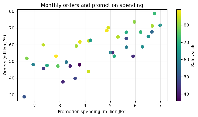 ### 結果の読み取り 販促費が大きい月ほど受注額も高い傾向ですが、同じ販促費でも訪問件数や偶然変動により幅があります。この幅を係数推定と将来予測に引き継ぐのがベイズ回帰です。相関だけで因果効果とは断定できない点にも注意します。 ## No.062：回帰係数に事前分布を設定する ### 実務での意味 少数データで「販促費1百万円あたり受注が数百百万円増える」といった非現実的な係数が出るのを抑え、過去の経験や業務上の上限をモデルへ明示します。 ### 分析・モデル化の考え方 説明変数を標準化したうえで、切片には $\alpha\sim\mathcal{N}(50,30)$、係数には $\beta_j\sim\mathcal{N}(0,15)$、誤差には $\sigma\sim\mathrm{HalfNormal}(15)$ を設定します。係数の正負を決め打ちしない弱情報事前分布です。事前予測チェックで、受注額として不自然な範囲を大量に生成しないか確かめます。 ### Pythonで確認する ```python features = ["promotion_million", "sales_visits"] X_mean, X_sd = sales[features].mean(), sales[features].std() X = ((sales[features] - X_mean) / X_sd).to_numpy() y = sales["orders_million"].to_numpy() prior_rng = np.random.default_rng(SEED + 1) alpha_prior = prior_rng.normal(50, 30, 4000) beta_prior = prior_rng.normal(0, 15, (4000, 2)) sigma_prior = np.abs(prior_rng.normal(0, 15, 4000)) mu_typical = alpha_prior # 標準化説明変数が0（平均的な月） y_prior = prior_rng.normal(mu_typical, sigma_prior) print(pd.Series(y_prior).quantile([0.025, 0.5, 0.975]).rename("prior orders")) ``` 0.025 -15.451 0.500 50.607 0.975 113.715 Name: prior orders, dtype: float64 ### 結果の読み取り 平均的な活動量の月について、事前予測は広いレンジを持ちます。これは「データを見る前には大きな不確実性があるが、桁違いの値は中心に置かない」という表現です。実務では過去3年のレンジや設備能力を基に、関係者と事前分布をレビューします。 ## No.063：ベイズ線形回帰を PyMC で実装する ### 実務での意味 仮定を再現可能なコードにし、モデル更新を属人的な表計算から定期実行可能な分析プロセスへ変えます。 ### 分析・モデル化の考え方 PyMC で尤度と事前分布を宣言し、NUTS により事後分布からサンプリングします。`r_hat` は複数チェーンの収束、`ess_bulk` は有効サンプルサイズの目安です。 ### Pythonで確認する ```python with pm.Model() as linear_model: alpha = pm.Normal("alpha", mu=50, sigma=30) beta = pm.Normal("beta", mu=0, sigma=15, shape=2) sigma = pm.HalfNormal("sigma", sigma=15) mu = alpha + pm.math.dot(X, beta) pm.Normal("orders", mu=mu, sigma=sigma, observed=y) linear_idata = pm.sample(700, tune=700, chains=2, cores=1, random_seed=SEED, target_accept=0.9, progressbar=False) linear_summary = az.summary(linear_idata, var_names=["alpha", "beta", "sigma"], hdi_prob=0.95, round_to=3) display(linear_summary) ``` Initializing NUTS using jitter+adapt_diag... Sequential sampling (2 chains in 1 job) NUTS: [alpha, beta, sigma] Sampling 2 chains for 700 tune and 700 draw iterations (1_400 + 1_400 draws total) took 16 seconds. We recommend running at least 4 chains for robust computation of convergence diagnostics <style scoped> .dataframe tbody tr th:only-of-type { vertical-align: middle; } .dataframe tbody tr th { vertical-align: top; } .dataframe thead th { text-align: right; } </style> <table border="1" class="dataframe"> <thead> <tr style="text-align: right;"> <th></th> <th>mean</th> <th>sd</th> <th>hdi_2.5%</th> <th>hdi_97.5%</th> <th>mcse_mean</th> <th>mcse_sd</th> <th>ess_bulk</th> <th>ess_tail</th> <th>r_hat</th> </tr> </thead> <tbody> <tr> <th>alpha</th> <td>57.116</td> <td>1.005</td> <td>54.979</td> <td>58.955</td> <td>0.029</td> <td>0.027</td> <td>1,248.667</td> <td>1,024.931</td> <td>1.000</td> </tr> <tr> <th>beta[0]</th> <td>8.216</td> <td>0.980</td> <td>6.286</td> <td>10.115</td> <td>0.028</td> <td>0.029</td> <td>1,268.098</td> <td>816.110</td> <td>1.001</td> </tr> <tr> <th>beta[1]</th> <td>4.974</td> <td>1.018</td> <td>3.251</td> <td>7.253</td> <td>0.028</td> <td>0.029</td> <td>1,313.071</td> <td>815.351</td> <td>1.000</td> </tr> <tr> <th>sigma</th> <td>5.904</td> <td>0.765</td> <td>4.544</td> <td>7.504</td> <td>0.026</td> <td>0.023</td> <td>917.377</td> <td>778.611</td> <td>1.002</td> </tr> </tbody> </table> ### 結果の読み取り `r_hat` が概ね 1.01 以下で、有効サンプルサイズが極端に小さくなければ、まず数値計算上の収束を確認できます。ただし収束はモデル妥当性の証明ではありません。残差、外れ値、時間依存、データ生成過程を別途点検します。 ## No.064：回帰係数の事後分布を確認する ### 実務での意味 「効果がある／ない」の二択ではなく、効果の大きさと向きにどの程度確信があるかを共有できます。 ### 分析・モデル化の考え方 標準化係数の事後分布について、95% HDI（最高事後密度区間）と正である確率を確認します。係数は他の説明変数を一定とした条件付きの関連です。 ### Pythonで確認する ```python beta_draws = linear_idata.posterior["beta"].stack(sample=("chain", "draw")).values coef_result = pd.DataFrame({ "feature": features, "posterior_mean": beta_draws.mean(axis=1), "hdi_2.5%": np.quantile(beta_draws, 0.025, axis=1), "hdi_97.5%": np.quantile(beta_draws, 0.975, axis=1), "P(beta>0)": (beta_draws > 0).mean(axis=1), }) display(coef_result) ``` <style scoped> .dataframe tbody tr th:only-of-type { vertical-align: middle; } .dataframe tbody tr th { vertical-align: top; } .dataframe thead th { text-align: right; } </style> <table border="1" class="dataframe"> <thead> <tr style="text-align: right;"> <th></th> <th>feature</th> <th>posterior_mean</th> <th>hdi_2.5%</th> <th>hdi_97.5%</th> <th>P(beta&gt;0)</th> </tr> </thead> <tbody> <tr> <th>0</th> <td>promotion_million</td> <td>8.216</td> <td>6.188</td> <td>10.107</td> <td>1.000</td> </tr> <tr> <th>1</th> <td>sales_visits</td> <td>4.974</td> <td>2.954</td> <td>7.050</td> <td>1.000</td> </tr> </tbody> </table> ### 結果の読み取り 正である確率が高く、区間がゼロから離れる変数ほど、正の関連を安定して観測できています。標準化係数なので活動量を1標準偏差増やしたときの比較ができます。一方、販促費と訪問件数が同時に決まる場合、施策の因果効果を得るには実験や交絡調整が必要です。 ## No.065：ベイズ回帰の信用区間を可視化する ### 実務での意味 予算案ごとの中心予測だけでなく、平均応答の信用区間を示すことで、経営と現場がリスク幅を共有できます。 ### 分析・モデル化の考え方 訪問件数を平均に固定し、販促費を変化させます。係数の事後標本ごとに期待受注額を計算し、その2.5・50・97.5パーセンタイルを描きます。これは平均応答の不確実性であり、個別月の偶然誤差は含みません。 ### Pythonで確認する ```python promo_grid = np.linspace(1.5, 7.0, 80) X_grid = np.column_stack([ (promo_grid - X_mean["promotion_million"]) / X_sd["promotion_million"], np.zeros_like(promo_grid), ]) alpha_draws = linear_idata.posterior["alpha"].stack(sample=("chain", "draw")).values mu_grid = alpha_draws[:, None] + beta_draws.T @ X_grid.T lo, med, hi = np.quantile(mu_grid, [0.025, 0.5, 0.975], axis=0) fig, ax = plt.subplots(figsize=(7, 4)) ax.scatter(sales["promotion_million"], y, alpha=0.55, label="Observed") ax.plot(promo_grid, med, color="C1", label="Posterior median") ax.fill_between(promo_grid, lo, hi, color="C1", alpha=0.25, label="95% credible interval") ax.set_title("Expected monthly orders at average sales visits") ax.set_xlabel("Promotion spending (million JPY)") ax.set_ylabel("Expected orders (million JPY)") ax.grid(True, alpha=0.3); ax.legend() plt.tight_layout(); plt.show() ``` 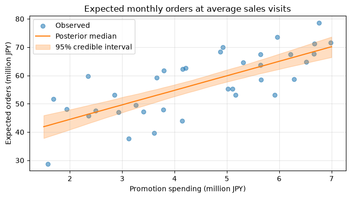 ### 結果の読み取り 帯が係数推定の不確実性です。観測が少ない領域への外挿ほど区間は一般に広がります。信用区間は「このモデルとデータの下で期待値が入る事後確率区間」であり、頻度論の信頼区間とは解釈が異なります。 ## No.066：ベイズ回帰で受注額を予測する ### 実務での意味 次月計画を単一値で置かず、下振れ・中央値・上振れを示し、資金繰りや生産能力のシナリオを作ります。 ### 分析・モデル化の考え方 次月を販促費5百万円、訪問70件とします。期待値の不確実性に観測誤差 $\sigma$ を加えた事後予測分布を作ります。予測区間は信用区間より広く、個別月のばらつきを含みます。 ### Pythonで確認する ```python next_x = np.array([(5.0 - X_mean["promotion_million"]) / X_sd["promotion_million"], (70 - X_mean["sales_visits"]) / X_sd["sales_visits"]]) sigma_draws = linear_idata.posterior["sigma"].stack(sample=("chain", "draw")).values next_mu = alpha_draws + beta_draws.T @ next_x pred_rng = np.random.default_rng(SEED + 2) next_orders = pred_rng.normal(next_mu, sigma_draws) q = np.quantile(next_orders, [0.025, 0.5, 0.975]) decision = pd.Series({"2.5%": q[0], "median": q[1], "97.5%": q[2], "P(orders < 50)": (next_orders < 50).mean()}) display(decision.to_frame("next-month prediction")) ``` <style scoped> .dataframe tbody tr th:only-of-type { vertical-align: middle; } .dataframe tbody tr th { vertical-align: top; } .dataframe thead th { text-align: right; } </style> <table border="1" class="dataframe"> <thead> <tr style="text-align: right;"> <th></th> <th>next-month prediction</th> </tr> </thead> <tbody> <tr> <th>2.5%</th> <td>49.198</td> </tr> <tr> <th>median</th> <td>61.317</td> </tr> <tr> <th>97.5%</th> <td>72.412</td> </tr> <tr> <th>P(orders &lt; 50)</th> <td>0.034</td> </tr> </tbody> </table> ### 結果の読み取り 中央値を基準計画、2.5%点を厳しい下振れケースとして利用できます。また「50百万円未満となる確率」は在庫や資金計画の発動条件に直結します。意思決定では予測精度だけでなく、過剰在庫と欠品の損失差を明示します。 ## No.067：ベイズロジスティック回帰を理解する ### 実務での意味 受注／失注のような二値結果をそのまま線形回帰すると、予測が0未満や1超になり得ます。ロジスティック回帰なら確率として案件評価できます。 ### 分析・モデル化の考え方 案件 $i$ の受注を $y_i\in\{0,1\}$ とし、 $$y_i\sim\mathrm{Bernoulli}(p_i),\qquad \mathrm{logit}(p_i)=\alpha+\boldsymbol{x}_i^\top\boldsymbol{\beta}$$ とします。係数を指数変換した $\exp(\beta)$ は、他条件一定で説明変数が1単位増えたときのオッズ比です。 ### Pythonで確認する ```python win_by_demo = deals.groupby("demo_done")["won"].agg(["count", "mean"]) win_by_demo.index = ["No demo", "Demo completed"] display(win_by_demo.rename(columns={"mean": "observed_win_rate"})) ``` <style scoped> .dataframe tbody tr th:only-of-type { vertical-align: middle; } .dataframe tbody tr th { vertical-align: top; } .dataframe thead th { text-align: right; } </style> <table border="1" class="dataframe"> <thead> <tr style="text-align: right;"> <th></th> <th>count</th> <th>observed_win_rate</th> </tr> </thead> <tbody> <tr> <th>No demo</th> <td>66</td> <td>0.318</td> </tr> <tr> <th>Demo completed</th> <td>94</td> <td>0.479</td> </tr> </tbody> </table> ### 結果の読み取り デモ実施案件の観測受注率は比較材料になりますが、案件金額やリード日数の構成差を調整していません。回帰モデルでは複数条件を同時に扱い、各案件の受注確率分布を得ます。なお、観測データからデモの因果効果を断定はできません。 ## No.068：購入確率をベイズロジスティック回帰で推定する ### 実務での意味 ここではB2Bの「購入」を見積案件の受注と読み替えます。確率順に案件を並べるだけでなく、案件金額との積で期待受注額を計算し、限られた営業工数を配分します。 ### 分析・モデル化の考え方 案件金額とリード日数を標準化し、デモ実施を0/1で投入します。弱情報事前分布 $\mathcal{N}(0,1.5)$ を使い、事後標本ごとに案件の受注確率を計算します。 ### Pythonで確認する ```python logit_cols = ["value_million", "demo_done", "lead_days"] logit_mean = deals[["value_million", "lead_days"]].mean() logit_sd = deals[["value_million", "lead_days"]].std() X_logit = np.column_stack([ (deals["value_million"] - logit_mean["value_million"]) / logit_sd["value_million"], deals["demo_done"], (deals["lead_days"] - logit_mean["lead_days"]) / logit_sd["lead_days"], ]) with pm.Model() as logit_model: a = pm.Normal("a", 0, 1.5) b = pm.Normal("b", 0, 1.5, shape=3) p = pm.Deterministic("p", pm.math.sigmoid(a + pm.math.dot(X_logit, b))) pm.Bernoulli("won", p=p, observed=deals["won"].to_numpy()) logit_idata = pm.sample(700, tune=700, chains=2, cores=1, random_seed=SEED + 3, target_accept=0.9, progressbar=False) p_draws = logit_idata.posterior["p"].stack(sample=("chain", "draw")).values deals_result = deals.copy() deals_result["win_prob"] = p_draws.mean(axis=1) deals_result["expected_orders_million"] = deals_result["value_million"] * deals_result["win_prob"] display(deals_result.nlargest(8, "expected_orders_million") [["value_million", "demo_done", "lead_days", "win_prob", "expected_orders_million"]]) ``` Initializing NUTS using jitter+adapt_diag... Sequential sampling (2 chains in 1 job) NUTS: [a, b] Sampling 2 chains for 700 tune and 700 draw iterations (1_400 + 1_400 draws total) took 89 seconds. We recommend running at least 4 chains for robust computation of convergence diagnostics <style scoped> .dataframe tbody tr th:only-of-type { vertical-align: middle; } .dataframe tbody tr th { vertical-align: top; } .dataframe thead th { text-align: right; } </style> <table border="1" class="dataframe"> <thead> <tr style="text-align: right;"> <th></th> <th>value_million</th> <th>demo_done</th> <th>lead_days</th> <th>win_prob</th> <th>expected_orders_million</th> </tr> </thead> <tbody> <tr> <th>143</th> <td>42.899</td> <td>1</td> <td>5</td> <td>0.554</td> <td>23.760</td> </tr> <tr> <th>156</th> <td>49.475</td> <td>1</td> <td>35</td> <td>0.394</td> <td>19.492</td> </tr> <tr> <th>93</th> <td>21.275</td> <td>1</td> <td>18</td> <td>0.538</td> <td>11.448</td> </tr> <tr> <th>144</th> <td>18.953</td> <td>1</td> <td>25</td> <td>0.503</td> <td>9.537</td> </tr> <tr> <th>149</th> <td>17.189</td> <td>1</td> <td>22</td> <td>0.525</td> <td>9.029</td> </tr> <tr> <th>11</th> <td>16.943</td> <td>1</td> <td>27</td> <td>0.496</td> <td>8.410</td> </tr> <tr> <th>41</th> <td>16.084</td> <td>1</td> <td>25</td> <td>0.510</td> <td>8.208</td> </tr> <tr> <th>76</th> <td>15.074</td> <td>1</td> <td>22</td> <td>0.531</td> <td>7.999</td> </tr> </tbody> </table> ### 結果の読み取り 確率が高くても小口の案件と、確率は中程度でも大型の案件では優先順位が変わります。期待受注額は有用な一次指標ですが、戦略顧客、粗利、フォロー所要時間、納期制約も加えて運用します。確率校正は時系列で検証し、人事評価へ短絡的に使わないことが重要です。 ## No.069：ベイズポアソン回帰を理解する ### 実務での意味 問い合わせ、故障、欠陥などの非負整数を扱います。稼働台数が増えると件数も増えるため、単純な平均だけでは要員計画を誤ります。 ### 分析・モデル化の考え方 週 $i$ の件数を $y_i$ として、 $$y_i\sim\mathrm{Poisson}(\lambda_i),\qquad \log\lambda_i=\alpha+\boldsymbol{x}_i^\top\boldsymbol{\beta}$$ とします。$\exp(\beta)$ は説明変数1単位増加に対する期待件数の倍率です。ポアソン分布は平均と分散が等しいため、過分散が強い場合は負の二項回帰を検討します。 ### Pythonで確認する ```python count_check = support["inquiries"].agg(["mean", "var", "min", "max"]) display(count_check.to_frame("inquiries")) fig, ax = plt.subplots(figsize=(7, 3.8)) ax.scatter(support["installed_100"], support["inquiries"], c=support["release_week"], cmap="coolwarm", alpha=0.75) ax.set_title("Weekly inquiries and installed base") ax.set_xlabel("Installed units (hundreds)") ax.set_ylabel("Inquiries per week") ax.grid(True, alpha=0.3) plt.tight_layout(); plt.show() ``` <style scoped> .dataframe tbody tr th:only-of-type { vertical-align: middle; } .dataframe tbody tr th { vertical-align: top; } .dataframe thead th { text-align: right; } </style> <table border="1" class="dataframe"> <thead> <tr style="text-align: right;"> <th></th> <th>inquiries</th> </tr> </thead> <tbody> <tr> <th>mean</th> <td>4.050</td> </tr> <tr> <th>var</th> <td>7.263</td> </tr> <tr> <th>min</th> <td>0.000</td> </tr> <tr> <th>max</th> <td>15.000</td> </tr> </tbody> </table> 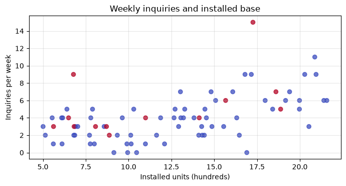 ### 結果の読み取り 稼働台数が多い週ほど件数が増える傾向と、リリース週の上振れが見えます。標本分散が平均を大きく超えるなら、説明変数不足、ゼロ過剰、週ごとの異質性も疑います。分布選択は業務プロセスの理解と事後予測チェックで判断します。 ## No.070：問い合わせ件数をベイズポアソン回帰で推定する ### 実務での意味 新リリース週の問い合わせ上振れを確率分布で予測し、一次対応要員、エスカレーション枠、外部委託枠を計画します。 ### 分析・モデル化の考え方 稼働台数を標準化し、リリース週フラグとともに対数リンクへ入れます。次週の期待件数だけでなく、ポアソンの偶然変動を含む事後予測分布を作り、処理能力超過確率を算出します。 ### Pythonで確認する ```python inst_mean, inst_sd = support["installed_100"].mean(), support["installed_100"].std() X_count = np.column_stack([(support["installed_100"] - inst_mean) / inst_sd, support["release_week"]]) with pm.Model() as count_model: ca = pm.Normal("ca", 0, 1.5) cb = pm.Normal("cb", 0, 1.0, shape=2) rate = pm.Deterministic("rate", pm.math.exp(ca + pm.math.dot(X_count, cb))) pm.Poisson("inquiries", mu=rate, observed=support["inquiries"].to_numpy()) count_idata = pm.sample(700, tune=700, chains=2, cores=1, random_seed=SEED + 4, target_accept=0.9, progressbar=False) ca_d = count_idata.posterior["ca"].stack(sample=("chain", "draw")).values cb_d = count_idata.posterior["cb"].stack(sample=("chain", "draw")).values next_count_x = np.array([(20 - inst_mean) / inst_sd, 1]) next_rate = np.exp(ca_d + cb_d.T @ next_count_x) count_rng = np.random.default_rng(SEED + 5) next_count = count_rng.poisson(next_rate) capacity = 8 count_plan = pd.Series({ "expected inquiries": next_count.mean(), "median": np.median(next_count), "95% prediction lower": np.quantile(next_count, 0.025), "95% prediction upper": np.quantile(next_count, 0.975), f"P(inquiries > {capacity})": (next_count > capacity).mean(), }) display(count_plan.to_frame("release-week plan")) fig, ax = plt.subplots(figsize=(7, 3.8)) bins = np.arange(next_count.min(), next_count.max() + 2) - 0.5 ax.hist(next_count, bins=bins, density=True, alpha=0.75, color="C2") ax.axvline(capacity, color="C3", linestyle="--", label=f"Capacity = {capacity}") ax.set_title("Posterior predictive inquiries: next release week") ax.set_xlabel("Inquiries per week") ax.set_ylabel("Probability") ax.grid(True, alpha=0.3); ax.legend() plt.tight_layout(); plt.show() ``` Initializing NUTS using jitter+adapt_diag... Sequential sampling (2 chains in 1 job) NUTS: [ca, cb] Sampling 2 chains for 700 tune and 700 draw iterations (1_400 + 1_400 draws total) took 33 seconds. We recommend running at least 4 chains for robust computation of convergence diagnostics <style scoped> .dataframe tbody tr th:only-of-type { vertical-align: middle; } .dataframe tbody tr th { vertical-align: top; } .dataframe thead th { text-align: right; } </style> <table border="1" class="dataframe"> <thead> <tr style="text-align: right;"> <th></th> <th>release-week plan</th> </tr> </thead> <tbody> <tr> <th>expected inquiries</th> <td>9.399</td> </tr> <tr> <th>median</th> <td>9.000</td> </tr> <tr> <th>95% prediction lower</th> <td>4.000</td> </tr> <tr> <th>95% prediction upper</th> <td>16.000</td> </tr> <tr> <th>P(inquiries &gt; 8)</th> <td>0.586</td> </tr> </tbody> </table> 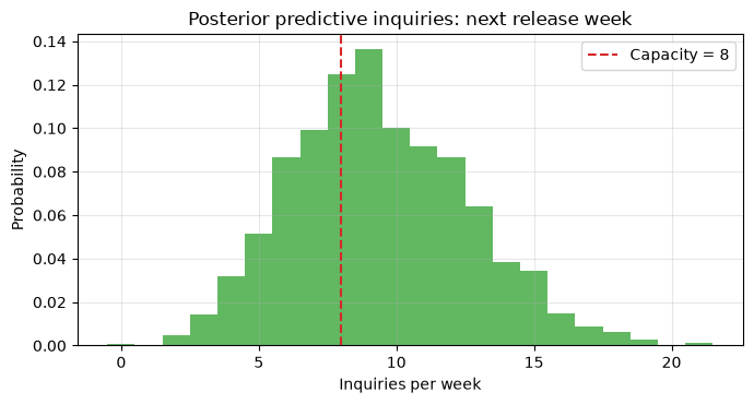 ### 結果の読み取り 95%予測区間は対応件数の現実的な幅、能力8件を超える確率は応援要員を確保する判断材料です。閾値は「超過1件の損失」と「余剰要員1人の費用」に基づいて決めます。件数だけでなく、難易度別の処理時間も次段階でモデル化します。 ## 対象ノックを通して見える実務上の示唆 1. 目的変数の型に合わせ、連続値には正規、二値にはベルヌーイ、件数にはポアソン尤度を選ぶ必要があります。 2. 点予測よりも、下振れ確率・能力超過確率・係数の符号確率が意思決定に役立ちます。 3. 事前分布は恣意性を隠すものではなく、データを見る前の想定を可視化し、関係者がレビューする対象です。 4. 予測上の関連と因果効果は別です。施策効果を知るなら、実験設計や交絡調整が必要です。 ## 実務導入する場合に必要なこと - **定義統一**：受注日、失注、問い合わせ起票などのKPI定義を固定する - **時点整合**：予測時点で利用可能だった説明変数だけを使い、情報漏洩を防ぐ - **検証**：時系列ホールドアウトで誤差、区間被覆率、確率校正を確認する - **診断**：MCMC収束、事後予測、外れ値、過分散、説明変数間相関を点検する - **運用**：閾値、再学習頻度、承認者、モデル停止条件を業務手順へ落とす - **ガバナンス**：モデルは担当者を補助するもので、評価や与信を自動確定しない ## まとめ No.061〜070では、ベイズ回帰を「係数を推定する技術」から「不確実性を含めて業務資源を配分する仕組み」へつなげました。受注額、受注確率、問い合わせ件数は異なるデータ型ですが、事前分布・尤度・事後分布・事後予測という共通の枠組みで整理できます。実務ではモデル精度だけでなく、予測を受けて誰が何を変えるのかまで設計することが成功条件です。 ## 法人向けのご相談 数理工房では、製造業向けのデータ分析研修、ベイズモデリング、需要・受注予測、意思決定ルール設計、PoCから運用定着までをご支援します。自社データに適した目的変数・尤度・事前分布の設計や、現場が説明可能なダッシュボードへの落とし込みもご相談いただけます。 > 📩 **お問い合わせ**: [surikobo.co.jp/contact](https://surikobo.co.jp/contact) > まずはお気軽にご相談ください。