
100本ノック / ベイズ統計 / データ分析のためのベイズ統計100本ノック
製造業のベイズ統計入門|需要予測・販促効果・異常検知をPythonで実践
不確実性を利益に変える:産業部品メーカーのベイズ需要予測と顧客・品質意思決定
本稿は「ベイズ統計100本ノック」第9章 No.081〜No.090 です。架空の産業部品メーカーを題材に、需要・売上の予測から販促評価、顧客行動、異常検知、経営報告までを一つの分析ストーリーとして扱います。点予測だけでなく、起こり得る範囲と意思決定確率を示すことが狙いです。
[!NOTE] 本資料は、数理工房 (もしくは代表である和山個人) が過去に企業研修において使用した notebook を企業様の許可を得て再構成・編集のうえ公開しています。
掲載データはすべて架空のものであり、実在する企業・工場・数値とは一切関係ありません。
はじめに:この記事で扱う製造業の実務課題
受注生産と見込生産が混在する工場では、需要の平均だけでは発注量、要員、在庫を決められません。さらに、展示会や技術広告の効果、代理店ごとの購入・離反、設備センサーの異常も、限られた観測から判断する必要があります。本稿ではベイズ更新により、過去知識と新しいデータを結合し、次の会議で使える確率へ変換します。
現場でよくある状況
- 月次予算が単一値で、欠品リスクと余剰在庫リスクが見えない
- 季節性と販促効果が混ざり、施策の寄与を説明できない
- 大口顧客と新規顧客を同じ基準で評価してしまう
- センサーの固定しきい値が誤報を多発させる
なぜこの問題は判断が難しいのか
標本が少なく、母数は直接観測できず、将来には観測ノイズも加わります。ベイズ統計では未知量を分布で表し、
として更新します。重要なのは「最もありそうな値」だけでなく、欠品、赤字、離反、異常といった事象の確率を意思決定に結び付けることです。
今回扱うノックの全体像
| No. | テーマ | 主な業務判断 |
|---|---|---|
| 081 | 需要予測 | 生産能力・材料手配 |
| 082 | 売上予測区間 | 予算・資金繰り |
| 083 | 季節性 | 繁忙期の先行生産 |
| 084 | キャンペーン効果 | 展示会施策の継続 |
| 085 | 広告効果の不確実性 | 媒体配分 |
| 086 | 購入確率 | 営業優先順位 |
| 087 | 購買回数 | 顧客別対応能力 |
| 088 | 離反確率 | 保全契約の更新活動 |
| 089 | ベイズ異常検知 | 点検・停止判断 |
| 090 | 業務レポート | 会議での合意形成 |
Python 環境の準備
外部データは使いません。乱数生成器を固定し、NumPy・pandas・SciPy・matplotlib のみで再現可能にします。ここでは日本語フォントへの依存を避けるためグラフ内のラベルは英語、本文の解釈は日本語とします。
import sys
import numpy as np
import pandas as pd
import matplotlib
import matplotlib.pyplot as plt
from scipy import stats

SEED = 20260712
rng = np.random.default_rng(SEED)
pd.set_option("display.precision", 3)
print(f"Python {sys.version.split()[0]}")
print(f"numpy {np.__version__} / pandas {pd.__version__} / matplotlib {matplotlib.__version__}")
Python 3.13.1
numpy 2.5.1 / pandas 3.0.3 / matplotlib 3.11.0架空データの作成
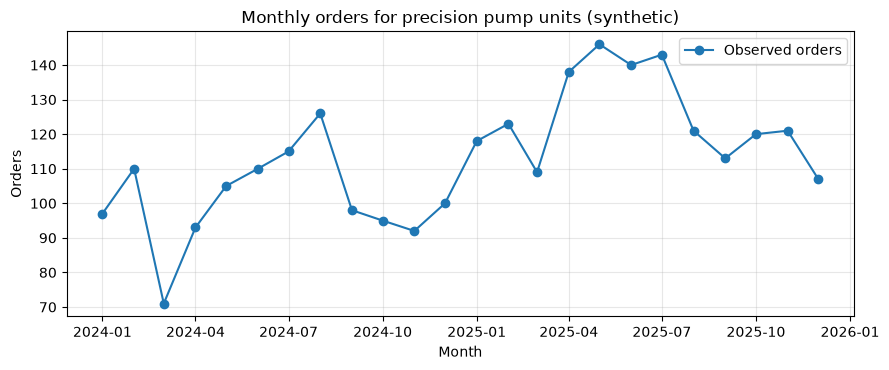
24か月分の精密ポンプユニットの受注と単価、展示会接触、広告費、顧客別購買・契約更新、設備振動を生成します。潜在的な増加傾向、夏冬の季節性、施策効果を含めますが、分析側はその正解を知らない前提です。
n_months = 24
dates = pd.date_range("2024-01-01", periods=n_months, freq="MS")
t = np.arange(n_months)
season = 1 + 0.18*np.sin(2*np.pi*(t-1)/12) + 0.08*np.cos(2*np.pi*t/6)
campaign = np.isin(t, [8, 9, 20, 21]).astype(int)
latent_demand = (92 + 1.4*t) * season * (1 + 0.10*campaign)
orders = rng.poisson(latent_demand)
unit_price = 128_000 + rng.normal(0, 3_500, n_months)
monthly = pd.DataFrame({"month": dates, "orders": orders, "unit_price_yen": unit_price.round(), "campaign": campaign})
monthly["sales_million_yen"] = monthly.orders * monthly.unit_price_yen / 1e6
display(monthly.tail(8))

fig, ax = plt.subplots(figsize=(9, 3.8))
ax.plot(monthly.month, monthly.orders, marker="o", label="Observed orders")
ax.set_title("Monthly orders for precision pump units (synthetic)")
ax.set_xlabel("Month"); ax.set_ylabel("Orders"); ax.grid(alpha=.3); ax.legend()
plt.tight_layout(); plt.show()| month | orders | unit_price_yen | campaign | sales_million_yen | |
|---|---|---|---|---|---|
| 16 | 2025-05-01 | 146 | 129462.0 | 0 | 18.901 |
| 17 | 2025-06-01 | 140 | 129769.0 | 0 | 18.168 |
| 18 | 2025-07-01 | 143 | 130565.0 | 0 | 18.671 |
| 19 | 2025-08-01 | 121 | 128417.0 | 0 | 15.538 |
| 20 | 2025-09-01 | 113 | 117132.0 | 1 | 13.236 |
| 21 | 2025-10-01 | 120 | 126404.0 | 1 | 15.168 |
| 22 | 2025-11-01 | 121 | 132070.0 | 0 | 15.980 |
| 23 | 2025-12-01 | 107 | 128970.0 | 0 | 13.800 |
No.081:ベイズ統計で需要予測を行う
実務での意味
直近6か月の需要水準を使って翌月の生産枠を検討します。少数月の単純平均を確定値とせず、過去の標準的な需要水準を事前分布として残すことで、突発的な一か月に過剰反応しにくくします。
分析・モデル化の考え方
月間需要 、需要率 ( は rate)とすると、事後分布は
です。次月需要は事後分布から を引き、さらにポアソン乱数を生成する事後予測で表します。
Pythonで確認する
recent = monthly.orders.tail(6).to_numpy()
a0, b0 = 100.0, 1.0
a_post, b_post = a0 + recent.sum(), b0 + len(recent)
lambda_draws = rng.gamma(a_post, 1/b_post, 50_000)
demand_next = rng.poisson(lambda_draws)
q = np.quantile(demand_next, [.05, .5, .95])
pd.DataFrame({"metric": ["posterior mean rate", "predictive P05", "predictive median", "predictive P95"],
"units": [lambda_draws.mean(), *q]}).round(1)| metric | units | |
|---|---|---|
| 0 | posterior mean rate | 117.9 |
| 1 | predictive P05 | 99.0 |
| 2 | predictive median | 118.0 |
| 3 | predictive P95 | 137.0 |
結果の読み取り
中央値は基準計画、P95 は欠品回避を重視した能力・材料確認の目安です。需要率の不確実性だけでなく来月固有の偶然変動も含むため、発注判断にはパラメータの信用区間ではなく事後予測区間を用います。
No.082:売上予測の予測区間を計算する
実務での意味
数量予測に単価の揺らぎを重ね、売上予算の達成確率と下振れ幅を見ます。これは資金繰りや残業枠を一つの強気シナリオだけで決めないために有効です。
分析・モデル化の考え方
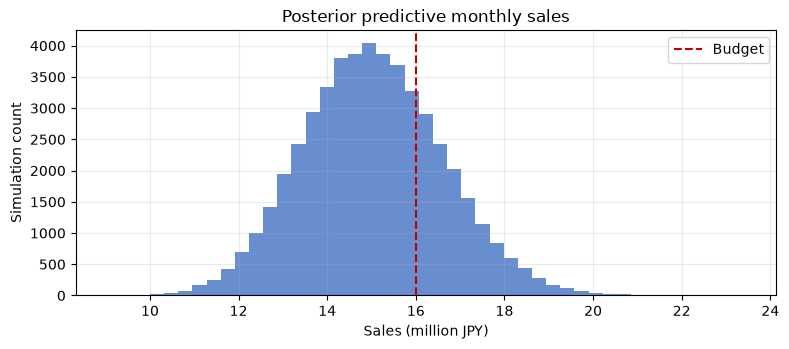
各シミュレーションで需要 と単価 を同時に生成し、 を計算します。非線形な積でもモンテカルロ法なら分布を直接要約できます。
Pythonで確認する
price_mu = monthly.unit_price_yen.tail(12).mean()
price_sd = monthly.unit_price_yen.tail(12).std(ddof=1)
price_next = np.maximum(rng.normal(price_mu, price_sd, len(demand_next)), 0)
sales_next = demand_next * price_next / 1e6
budget = 16.0
summary_082 = pd.Series({"P05 (million yen)": np.quantile(sales_next,.05),
                         "median (million yen)": np.median(sales_next),
                         "P95 (million yen)": np.quantile(sales_next,.95),
                         "P(sales >= budget)": np.mean(sales_next >= budget)})
display(summary_082.round(3))
fig, ax = plt.subplots(figsize=(8,3.6)); ax.hist(sales_next,bins=45,color="#4472C4",alpha=.8)
ax.axvline(budget,color="#C00000",ls="--",label="Budget")
ax.set_title("Posterior predictive monthly sales"); ax.set_xlabel("Sales (million JPY)"); ax.set_ylabel("Simulation count")
ax.grid(alpha=.25); ax.legend(); plt.tight_layout(); plt.show()
P05 (million yen) 12.509
median (million yen) 14.988
P95 (million yen) 17.713
P(sales >= budget) 0.267
dtype: float64
結果の読み取り
予算達成確率は「達成する/しない」の断定よりも、営業・製造・財務が共通のリスク認識を持つ材料になります。P05 をストレスケース、中央値を標準ケース、P95 を上振れケースとして資金・能力計画を並べられます。
No.083:季節性を考慮したベイズモデルを作る
実務での意味
繁忙期を単なる異常値として均してしまうと先行生産が遅れます。月別係数を部分的に全体平均へ縮約し、データが少ない月の季節指数を安定化します。
分析・モデル化の考え方
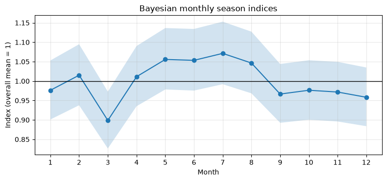
説明を明快にするため、各月の受注率に Gamma 事前分布を置く共役モデルを使います。月 の観測について とし、共通事前分布が過度な月別変動を抑えます。
Pythonで確認する
season_rows=[]
global_mean=monthly.orders.mean()
for m,g in monthly.assign(month_num=monthly.month.dt.month).groupby("month_num"):
    ap, bp = global_mean*2 + g.orders.sum(), 2 + len(g)
    draws=rng.gamma(ap,1/bp,20_000)
    season_rows.append([m,draws.mean()/global_mean,*np.quantile(draws/global_mean,[.05,.95])])
season_post=pd.DataFrame(season_rows,columns=["month","season_index","p05","p95"])
display(season_post.round(3))
fig,ax=plt.subplots(figsize=(8,3.8)); ax.plot(season_post.month,season_post.season_index,marker="o")
ax.fill_between(season_post.month,season_post.p05,season_post.p95,alpha=.2)
ax.axhline(1,color="black",lw=1); ax.set_title("Bayesian monthly season indices")
ax.set_xlabel("Month"); ax.set_ylabel("Index (overall mean = 1)"); ax.set_xticks(range(1,13)); ax.grid(alpha=.3)
plt.tight_layout(); plt.show()| month | season_index | p05 | p95 | |
|---|---|---|---|---|
| 0 | 1 | 0.976 | 0.901 | 1.053 |
| 1 | 2 | 1.015 | 0.938 | 1.095 |
| 2 | 3 | 0.899 | 0.826 | 0.973 |
| 3 | 4 | 1.011 | 0.935 | 1.090 |
| 4 | 5 | 1.056 | 0.978 | 1.136 |
| 5 | 6 | 1.053 | 0.976 | 1.134 |
| 6 | 7 | 1.071 | 0.992 | 1.153 |
| 7 | 8 | 1.046 | 0.968 | 1.127 |
| 8 | 9 | 0.967 | 0.893 | 1.044 |
| 9 | 10 | 0.976 | 0.900 | 1.054 |
| 10 | 11 | 0.972 | 0.896 | 1.050 |
| 11 | 12 | 0.958 | 0.884 | 1.035 |
結果の読み取り
指数が1を上回る月は平常月より需要が多い候補です。ただし帯が広い月は確証が弱いため、指数の順位だけで設備投資せず、納期情報や受注残と組み合わせて先行手配します。
No.084:キャンペーン効果をベイズ推定する
実務での意味
展示会後の技術相談が案件化した割合を、通常の営業接触と比較します。「差が正か」だけでなく、実務上必要な改善幅を超える確率を評価します。
分析・モデル化の考え方
案件化率に独立な 事前分布を置きます。成功 、失敗 の観測後は です。2群の事後標本差から優越確率と最小有効差を超える確率を求めます。
Pythonで確認する
campaign_leads, campaign_wins = 85, 25
usual_leads, usual_wins = 110, 22
p_c = rng.beta(1+campaign_wins,1+campaign_leads-campaign_wins,50_000)
p_u = rng.beta(1+usual_wins,1+usual_leads-usual_wins,50_000)
lift = p_c-p_u
pd.Series({"campaign posterior mean":p_c.mean(),"usual posterior mean":p_u.mean(),
           "P(campaign > usual)":np.mean(lift>0),"P(lift > 5pt)":np.mean(lift>.05),
           "lift P05":np.quantile(lift,.05),"lift P95":np.quantile(lift,.95)}).round(3)
campaign posterior mean 0.299
usual posterior mean 0.205
P(campaign > usual) 0.936
P(lift > 5pt) 0.760
lift P05 -0.008
lift P95 0.195
dtype: float64結果の読み取り
優越確率が高くても、5ポイント以上の改善確率が低ければ、会場費・技術者工数を回収できない可能性があります。最低有効差は分析後に都合よく決めず、粗利と施策費から事前に合意します。
No.085:広告効果の不確実性を評価する
実務での意味
技術媒体への広告費と問い合わせ増加の関係を推定します。係数の符号だけでなく、追加100万円が生む問い合わせ数の幅を媒体配分に使います。
分析・モデル化の考え方
正規線形モデル を考え、、既知の を仮定すると事後分布も正規分布です。広告費と季節要因を同時に入れ、交絡を減らします。
Pythonで確認する
n=30
ad_spend=rng.uniform(0.4,2.2,n)
busy=np.sin(2*np.pi*np.arange(n)/12)
inquiries=18+5.2*ad_spend+3.0*busy+rng.normal(0,3.5,n)
X=np.column_stack([np.ones(n),ad_spend,busy]); sigma=3.5; tau=10.0
V=np.linalg.inv(X.T@X/sigma**2+np.eye(3)/tau**2)
m=V@(X.T@inquiries/sigma**2)
beta=rng.multivariate_normal(m,V,50_000)
effect=beta[:,1]
pd.Series({"inquiries per +1M JPY (mean)":effect.mean(),"P05":np.quantile(effect,.05),
           "P95":np.quantile(effect,.95),"P(effect > 0)":np.mean(effect>0)}).round(3)
inquiries per +1M JPY (mean) 4.430
P05 2.117
P95 6.735
P(effect > 0) 0.999
dtype: float64結果の読み取り
効果の信用区間が広い場合、全額投入よりも小規模な追加テストに価値があります。係数は相関に基づくため、媒体選択や営業活動の未観測交絡が残る点をレポートに明記します。
No.086:顧客の購入確率をベイズ推定する
実務での意味
代理店別の見積提出後の購入率を推定し、営業フォローを優先します。件数の少ない代理店を0%・100%と断定しないことが重要です。
分析・モデル化の考え方
過去全体を弱い 事前分布として各社の二項データを更新します。事後平均は観測率と事前平均の加重平均になり、小標本ほど強く縮約されます。
Pythonで確認する
customers=pd.DataFrame({"dealer":["A","B","C","D","E"],"quotes":[42,18,8,30,5],"purchases":[20,6,4,9,4]})
a0,b0=2,3
customers["raw_rate"]=customers.purchases/customers.quotes
customers["posterior_mean"]=(a0+customers.purchases)/(a0+b0+customers.quotes)
customers["P(rate>40%)"]=[1-stats.beta.cdf(.4,a0+s,b0+n-s) for n,s in zip(customers.quotes,customers.purchases)]
display(customers.round(3).sort_values("P(rate>40%)",ascending=False))| dealer | quotes | purchases | raw_rate | posterior_mean | P(rate>40%) | |
|---|---|---|---|---|---|---|
| 4 | E | 5 | 4 | 0.800 | 0.600 | 0.901 |
| 0 | A | 42 | 20 | 0.476 | 0.468 | 0.825 |
| 2 | C | 8 | 4 | 0.500 | 0.462 | 0.665 |
| 1 | B | 18 | 6 | 0.333 | 0.348 | 0.290 |
| 3 | D | 30 | 9 | 0.300 | 0.314 | 0.138 |
結果の読み取り
生の購入率だけなら小標本のE社が最上位になりますが、事後確率は証拠量も反映します。営業優先順位は購入確率に加えて案件粗利、移動・対応コスト、戦略的重要性と組み合わせます。
No.087:購買回数をガンマ・ポアソンモデルで推定する
実務での意味
保守部品の顧客別発注頻度を更新し、補充頻度と担当者の対応能力を決めます。短い観測期間のゼロ回も「今後ずっとゼロ」とは扱いません。
分析・モデル化の考え方
顧客の月間発注率 、観測期間 の回数 なら、事後分布は です。
Pythonで確認する
freq=pd.DataFrame({"customer":["K1","K2","K3","K4"],"months":[6,12,4,9],"orders":[9,11,1,18]})
a0,b0=2,2
freq["observed_per_month"]=freq.orders/freq.months
freq["posterior_rate"]=(a0+freq.orders)/(b0+freq.months)
freq["next_3m_orders"] = 3*freq.posterior_rate
display(freq.round(2))| customer | months | orders | observed_per_month | posterior_rate | next_3m_orders | |
|---|---|---|---|---|---|---|
| 0 | K1 | 6 | 9 | 1.50 | 1.38 | 4.12 |
| 1 | K2 | 12 | 11 | 0.92 | 0.93 | 2.79 |
| 2 | K3 | 4 | 1 | 0.25 | 0.50 | 1.50 |
| 3 | K4 | 9 | 18 | 2.00 | 1.82 | 5.45 |
結果の読み取り
K3のような短期・少数観測は全体知識へ縮約され、過小な在庫設定を避けられます。合計需要を作る際は各顧客の事後予測を足し合わせ、リードタイム中の分布として安全在庫へ接続します。
No.088:離反確率をベイズ的に考える
実務での意味
保全契約の更新失敗を離反とし、重点フォロー対象を決めます。離反率の高さだけでなく、契約金額を掛けた期待損失で優先順位を付けます。
分析・モデル化の考え方
セグメント別離反率を Beta–Binomial で更新し、 を計算します。期待損失は概算として契約金額×事後離反率で示します。
Pythonで確認する
churn=pd.DataFrame({"segment":["Key","Growth","Standard"],"renewals":[35,48,80],"churned":[2,8,18],"annual_value_myen":[3.2,1.4,.6]})
a0,b0=2,18
churn["posterior_churn"]=(a0+churn.churned)/(a0+b0+churn.renewals)
churn["P(churn>15%)"]=[1-stats.beta.cdf(.15,a0+s,b0+n-s) for n,s in zip(churn.renewals,churn.churned)]
churn["expected_loss_myen_each"]=churn.annual_value_myen*churn.posterior_churn
display(churn.round(3))| segment | renewals | churned | annual_value_myen | posterior_churn | P(churn>15%) | expected_loss_myen_each | |
|---|---|---|---|---|---|---|---|
| 0 | Key | 35 | 2 | 3.2 | 0.073 | 0.030 | 0.233 |
| 1 | Growth | 48 | 8 | 1.4 | 0.147 | 0.441 | 0.206 |
| 2 | Standard | 80 | 18 | 0.6 | 0.200 | 0.902 | 0.120 |
結果の読み取り
離反確率が低い重要顧客でも契約額が大きければ期待損失は無視できません。一方、介入可能性を確かめず全件に値引きすると利益を損なうため、原因分類と施策別効果検証が必要です。
No.089:異常検知にベイズ的なしきい値を使う
実務での意味
組立設備の振動RMS値について、正常時データから次の観測の分布を作り、固定値ではなく正常状態の不確実性を含むしきい値で点検を判断します。
分析・モデル化の考え方
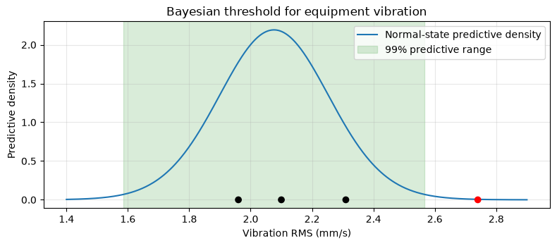
正常値を正規分布とし、平均・分散が未知の場合の事後予測は Student の 分布になります。新観測 の両側事後予測確率が小さければ異常候補です。
Pythonで確認する
normal_vibration=rng.normal(2.05,.16,40)
new_vibration=np.array([2.10,2.31,2.74,1.96])
n=len(normal_vibration); mean=normal_vibration.mean(); s=normal_vibration.std(ddof=1)
pred_scale=s*np.sqrt(1+1/n); dist=stats.t(df=n-1,loc=mean,scale=pred_scale)
lower,upper=dist.ppf([.005,.995])
tail=2*np.minimum(dist.cdf(new_vibration),1-dist.cdf(new_vibration))
result_089=pd.DataFrame({"vibration":new_vibration,"two_sided_predictive_p":tail,"alert":tail<.01})
display(result_089.round(5)); print(f"99% posterior predictive interval: [{lower:.3f}, {upper:.3f}]")
fig,ax=plt.subplots(figsize=(8,3.6)); x=np.linspace(1.4,2.9,500); ax.plot(x,dist.pdf(x),label="Normal-state predictive density")
ax.axvspan(lower,upper,alpha=.15,color="green",label="99% predictive range"); ax.scatter(new_vibration,np.zeros_like(new_vibration),c=np.where(tail<.01,"red","black"),zorder=3)
ax.set_title("Bayesian threshold for equipment vibration"); ax.set_xlabel("Vibration RMS (mm/s)"); ax.set_ylabel("Predictive density")
ax.grid(alpha=.3); ax.legend(); plt.tight_layout(); plt.show()| vibration | two_sided_predictive_p | alert | |
|---|---|---|---|
| 0 | 2.10 | 8.953e-01 | False |
| 1 | 2.31 | 2.033e-01 | False |
| 2 | 2.74 | 7.200e-04 | True |
| 3 | 1.96 | 5.247e-01 | False |
99% posterior predictive interval: [1.586, 2.566]
結果の読み取り
赤い点は正常モデルでは起こりにくく、点検候補です。ただし異常確率そのものではなく「正常ならどれほど珍しいか」を見ています。停止判断には故障事前確率、見逃し・誤報コスト、複数センサー、連続回数を加えます。
No.090:ベイズ分析結果を業務レポートにまとめる
実務での意味
モデルの係数一覧ではなく、意思決定、確率、金額、推奨アクション、留保条件を1枚にまとめます。分析者以外が再現可能な判断規則を持つことが目的です。
分析・モデル化の考え方
報告では (1)問い、(2)データ期間、(3)事前分布、(4)事後予測、(5)意思決定基準、(6)感度・限界を分離します。確率だけで自動決定せず、損失関数と業務制約を併記します。
Pythonで確認する
report=pd.DataFrame([
 ["Next-month capacity",f"P95 demand = {np.quantile(demand_next,.95):.0f} units","Check material/capacity at P95","Demand model uses recent 6 months"],
 ["Sales budget",f"P(>= JPY {budget:.0f}M) = {np.mean(sales_next>=budget):.1%}","Prepare P05 cash scenario","Price and quantity simulated"],
 ["Campaign",f"P(lift > 5pt) = {np.mean(lift>.05):.1%}","Compare expected margin with cost","Observational follow-up may differ"],
 ["Equipment alert",f"{result_089.alert.sum()} of {len(result_089)} readings","Inspect alert readings","Confirm with other sensors"]],
 columns=["decision","evidence","recommended_action","caveat"])
display(report)| decision | evidence | recommended_action | caveat | |
|---|---|---|---|---|
| 0 | Next-month capacity | P95 demand = 137 units | Check material/capacity at P95 | Demand model uses recent 6 months |
| 1 | Sales budget | P(>= JPY 16M) = 26.7% | Prepare P05 cash scenario | Price and quantity simulated |
| 2 | Campaign | P(lift > 5pt) = 76.0% | Compare expected margin with cost | Observational follow-up may differ |
| 3 | Equipment alert | 1 of 4 readings | Inspect alert readings | Confirm with other sensors |
結果の読み取り
同じ表に「証拠」「行動」「留保」を並べることで、確率が独り歩きするのを防ぎます。更新日、コード版、データ抽出条件、承認者も本番レポートに付け、翌月に予測と実績を照合します。
対象ノックを通して見える実務上の示唆
ベイズ分析の価値は高度な分布名ではなく、情報が少ないときも過去知識を明示的に使い、新データで継続更新し、意思決定に必要な確率を直接計算できる点にあります。需要、顧客、品質を別々の点推定で管理するより、「どの損失を避けたいか」に合わせて予測分布を要約する方が、部門間の判断基準を揃えやすくなります。
実務導入する場合に必要なこと
- 意思決定と損失の定義:欠品、余剰、誤報、見逃しの費用を合意する
- データ生成過程の確認:欠測、打切り、価格改定、施策対象選定を記録する
- 事前分布のレビュー:根拠と感度分析を残し、都合のよい調整を防ぐ
- 妥当性確認:事後予測チェック、時系列バックテスト、校正を定期実施する
- 運用設計:更新頻度、責任者、例外処理、モデル停止条件を決める
まとめ
No.081〜No.090 では、共役モデルとシミュレーションを中心に、製造業の需要・売上・施策・顧客・設備の不確実性を確率として表しました。次の一歩は、貴社固有の損失と制約を定義し、予測精度だけでなく意思決定後の利益・サービス水準・安全性で評価することです。
法人向けのご相談
需要予測、在庫・生産計画、販促効果検証、予知保全の導入では、モデル作成に加えてデータ定義、現場の判断規則、運用・教育まで一体で設計する必要があります。数理工房では、PoC設計、分析基盤、社内研修、意思決定プロセスへの実装をご支援します。
📩 お問い合わせ: surikobo.co.jp/contact
まずはお気軽にご相談ください。