Turning Uncertainty into Profit: Bayesian Demand Forecasting and Customer Quality Decision-Making for Industrial Component Manufacturers

This article is from Chapter 9 No.081–No.090 of ‘100 Exercises in Bayesian Statistics.’ Using a fictional industrial parts manufacturer as the subject, it handles everything from demand and sales forecasting to promotional evaluations, customer behavior, anomaly detection, and management reporting as a single analytical story. The aim is not only to predict points but also to show Possible Range and Decision Probability.

[!NOTE] This material is a notebook previously used by Surikoubo (or personally by the representative, Kazuyama), and has been reconstructed, edited, and published with the company’s permission.
All data listed is fictional and has no relation whatsoever to real companies, factories, or figures.

Introduction: Practical Challenges in Manufacturing Covered in This Article

In factories where made-to-order and forecast-based production coexist, average demand alone cannot determine order volume, personnel, or inventory. Furthermore, the effectiveness of exhibitions and technical advertising, purchases and defects by agents, and abnormalities in equipment sensors all need to be judged based on limited observations. In this article, we combine past knowledge with new data through Bayesian updates and convert them into probabilities that can be used in the next meeting.

Common situations on site

• Monthly budgets are single-valued, with no visible risk of stockout or excess inventory
• Seasonality and promotional effects mix, making it impossible to explain the contribution of the initiative.
• Evaluating large and new clients by the same standards
• Fixed sensor thresholds cause frequent false alarms

Why is this issue so difficult to judge?

With few samples, the population cannot be directly observed, and observational noise may be added in the future. In Bayesian statistics, unknown quantities are expressed as distributions,

$p(\theta\mid y)=\frac{p(y\mid\theta)p(\theta)}{p(y)}\propto p(y\mid\theta)p(\theta)$

This is the update. What matters is not just the “most likely value,” but also linking the probability of events such as out-of-stock, deficits, defections, and anomalies to decision-making.

Overview of Exercise covered this time

No.	Theme	Main Business Decisions
081	Demand forecasting	Production Capacity and Material Arrangement
082	Sales forecast segments	Budget and Cash Flow
083	seasonal	Early production during busy periods
084	Campaign Effects	Continued exhibition initiatives
085	Uncertainty in advertising effectiveness	Media Allocation
086	Purchase Probability	Business Priorities
087	Number of purchases	Customer-specific response capabilities
088	defection probability	Conservation contract renewal activities
089	Bayesian anomaly detection	Inspection and Stop Decisions
090	Business Report	Consensus Building in Meetings

Preparing the Python environment

No external data is used. Fix the random number generator and make it reproduce using only NumPy, pandas, SciPy, and matplotlib. To avoid relying on Japanese fonts, labels in the graph are in English, and the interpretation of the text is in Japanese.

import sys
import numpy as np
import pandas as pd
import matplotlib
import matplotlib.pyplot as plt
from scipy import stats

SEED = 20260712
rng = np.random.default_rng(SEED)
pd.set_option("display.precision", 3)
print(f"Python {sys.version.split()[0]}")
print(f"numpy {np.__version__} / pandas {pd.__version__} / matplotlib {matplotlib.__version__}")

Python 3.13.1
numpy 2.5.1 / pandas 3.0.3 / matplotlib 3.11.0

Creation of Fictional Data

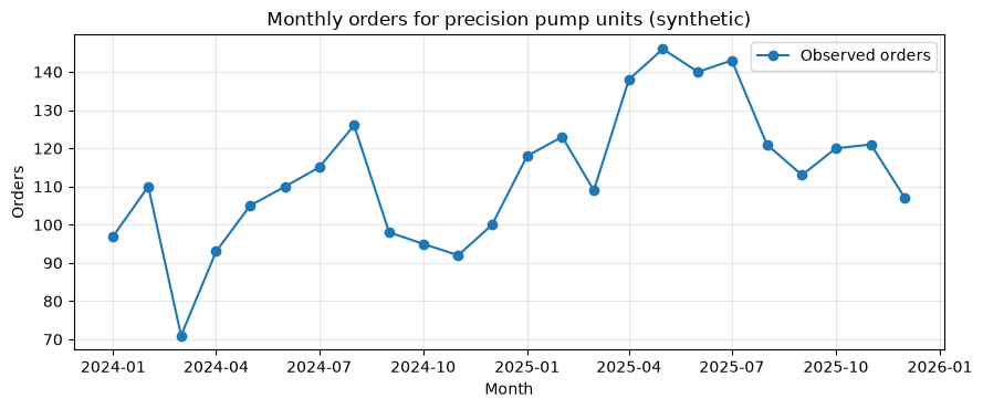
We generate 24 months’ worth of precision pump unit orders and unit prices, exhibition contacts, advertising expenses, customer-specific purchases and contract renewals, and equipment vibration. It includes potential growth trends, seasonality in summer and winter, and policy effects, but analysts assume they do not know the correct answers.

n_months = 24
dates = pd.date_range("2024-01-01", periods=n_months, freq="MS")
t = np.arange(n_months)
season = 1 + 0.18*np.sin(2*np.pi*(t-1)/12) + 0.08*np.cos(2*np.pi*t/6)
campaign = np.isin(t, [8, 9, 20, 21]).astype(int)
latent_demand = (92 + 1.4*t) * season * (1 + 0.10*campaign)
orders = rng.poisson(latent_demand)
unit_price = 128_000 + rng.normal(0, 3_500, n_months)
monthly = pd.DataFrame({"month": dates, "orders": orders, "unit_price_yen": unit_price.round(), "campaign": campaign})
monthly["sales_million_yen"] = monthly.orders * monthly.unit_price_yen / 1e6
display(monthly.tail(8))

fig, ax = plt.subplots(figsize=(9, 3.8))
ax.plot(monthly.month, monthly.orders, marker="o", label="Observed orders")
ax.set_title("Monthly orders for precision pump units (synthetic)")
ax.set_xlabel("Month"); ax.set_ylabel("Orders"); ax.grid(alpha=.3); ax.legend()
plt.tight_layout(); plt.show()

	month	orders	unit_price_yen	campaign	sales_million_yen
16	2025-05-01	146	129462.0	0	18.901
17	2025-06-01	140	129769.0	0	18.168
18	2025-07-01	143	130565.0	0	18.671
19	2025-08-01	121	128417.0	0	15.538
20	2025-09-01	113	117132.0	1	13.236
21	2025-10-01	120	126404.0	1	15.168
22	2025-11-01	121	132070.0	0	15.980
23	2025-12-01	107	128970.0	0	13.800

No.081: Demand Forecasting Using Bayesian Statistics

Meaning in Practice

We use the demand levels from the past six months to consider production quotas for the following month. By not using the simple average of a few months as a fixed value and instead preserving past standard demand levels as a preliminary distribution, it is less likely to overreact to sudden one-month events.

Approach to Analysis and Modeling

If monthly demand $y_i\sim\mathrm{Poisson}(\lambda)$ and demand rate $\lambda\sim\mathrm{Gamma}(a_0,b_0)$ ($b$ is rate), the posterior distribution is

$\lambda\mid y\sim\mathrm{Gamma}\left(a_0+\sum y_i,\ b_0+n\right)$

That’s right. Next month’s demand is represented by subtracting $\lambda$ from the posterior distribution and generating a Poisson random number through a post-event forecast.

Check with Python

recent = monthly.orders.tail(6).to_numpy()
a0, b0 = 100.0, 1.0
a_post, b_post = a0 + recent.sum(), b0 + len(recent)
lambda_draws = rng.gamma(a_post, 1/b_post, 50_000)
demand_next = rng.poisson(lambda_draws)
q = np.quantile(demand_next, [.05, .5, .95])
pd.DataFrame({"metric": ["posterior mean rate", "predictive P05", "predictive median", "predictive P95"],
              "units": [lambda_draws.mean(), *q]}).round(1)

	metric	units
0	posterior mean rate	117.9
1	predictive P05	99.0
2	predictive median	118.0
3	predictive P95	137.0

Reading the results

The median is the standard plan, and P95 is a reference for checking capacity and materials, emphasizing shortage avoidance. Because there is not only uncertainty in demand rates but also accidental fluctuations unique to the next month, order decisions use the post-Prediction interval rather than the parameter’s credit range.

No.082: Calculating the forecast segment for sales forecasts

Meaning in Practice

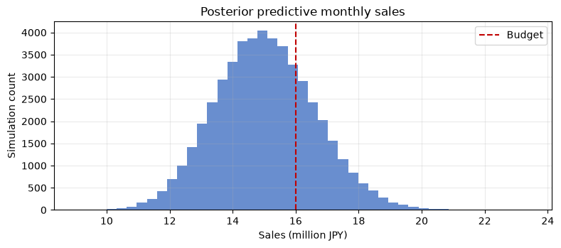
We overlay fluctuations in unit prices on volume forecasts to assess the probability and downside of achieving sales budgets. This is effective because you don’t have to decide on cash flow or overtime limits based solely on one bullish scenario.

Approach to Analysis and Modeling

Each simulation simultaneously generates demand $\tilde y$ and unit price $\tilde p$, and calculates $\tilde R=\tilde y\tilde p$. Even nonlinear products can be directly summarized using the Monte Carlo method.

Check with Python

price_mu = monthly.unit_price_yen.tail(12).mean()
price_sd = monthly.unit_price_yen.tail(12).std(ddof=1)
price_next = np.maximum(rng.normal(price_mu, price_sd, len(demand_next)), 0)
sales_next = demand_next * price_next / 1e6
budget = 16.0
summary_082 = pd.Series({"P05 (million yen)": np.quantile(sales_next,.05),
                         "median (million yen)": np.median(sales_next),
                         "P95 (million yen)": np.quantile(sales_next,.95),
                         "P(sales >= budget)": np.mean(sales_next >= budget)})
display(summary_082.round(3))
fig, ax = plt.subplots(figsize=(8,3.6)); ax.hist(sales_next,bins=45,color="#4472C4",alpha=.8)
ax.axvline(budget,color="#C00000",ls="--",label="Budget")
ax.set_title("Posterior predictive monthly sales"); ax.set_xlabel("Sales (million JPY)"); ax.set_ylabel("Simulation count")
ax.grid(alpha=.25); ax.legend(); plt.tight_layout(); plt.show()

P05 (million yen)       12.509
median (million yen)    14.988
P95 (million yen)       17.713
P(sales >= budget)       0.267
dtype: float64

Reading the results

The probability of achieving the budget is more important than the definitive judgment of ‘achieve/not achieved,’ and sales, manufacturing, and finance share a common risk perception. You can arrange funding and capability plans with P05 as a stress case, a median as a standard case, and P95 as an upside case.

No.083: Creating a Bayesian Model Considering Seasonality

Meaning in Practice

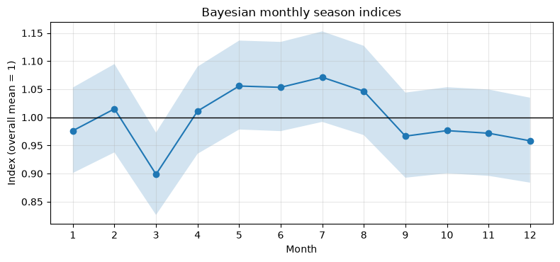
If you treat the busy period as mere abnormal values, early production will be delayed. Monthly coefficients are partially reduced to overall averages to stabilize seasonal indices for months with less data.

Approach to Analysis and Modeling

To clarify the explanation, a conjugate model is used, which places a Gamma pre-distribution on the order rate for each month. Regarding the observation of the monthly $m$, set it to $y_{m,j}\sim\mathrm{Poisson}(\lambda_m)$ to suppress excessive monthly variation in the common pre-distribution.

Check with Python

season_rows=[]
global_mean=monthly.orders.mean()
for m,g in monthly.assign(month_num=monthly.month.dt.month).groupby("month_num"):
    ap, bp = global_mean*2 + g.orders.sum(), 2 + len(g)
    draws=rng.gamma(ap,1/bp,20_000)
    season_rows.append([m,draws.mean()/global_mean,*np.quantile(draws/global_mean,[.05,.95])])
season_post=pd.DataFrame(season_rows,columns=["month","season_index","p05","p95"])
display(season_post.round(3))
fig,ax=plt.subplots(figsize=(8,3.8)); ax.plot(season_post.month,season_post.season_index,marker="o")
ax.fill_between(season_post.month,season_post.p05,season_post.p95,alpha=.2)
ax.axhline(1,color="black",lw=1); ax.set_title("Bayesian monthly season indices")
ax.set_xlabel("Month"); ax.set_ylabel("Index (overall mean = 1)"); ax.set_xticks(range(1,13)); ax.grid(alpha=.3)
plt.tight_layout(); plt.show()

	month	season_index	p05	p95
0	1	0.976	0.901	1.053
1	2	1.015	0.938	1.095
2	3	0.899	0.826	0.973
3	4	1.011	0.935	1.090
4	5	1.056	0.978	1.136
5	6	1.053	0.976	1.134
6	7	1.071	0.992	1.153
7	8	1.046	0.968	1.127
8	9	0.967	0.893	1.044
9	10	0.976	0.900	1.054
10	11	0.972	0.896	1.050
11	12	0.958	0.884	1.035

Reading the results

Months with an index above 1 are candidates with higher demand than in regular months. However, months with wide bands have weaker convictions, so we do not invest in equipment based solely on index rankings, but arrange ahead by combining delivery date information and backlog with orders.

No.084: Estimating Campaign Effectiveness by Bayesian

Meaning in Practice

We compare the proportion of post-exhibition technical consultations that have become cases with regular sales contacts. We evaluate not only whether the difference is correct, but also the probability that the range of improvement required in practice exceeds the threshold required.

Approach to Analysis and Modeling

Place a $\mathrm{Beta}(1,1)$ pre-distribution independent of the case conversion rate. After observing $s$ success and failure $f$, it is $\mathrm{Beta}(1+s,1+f)$. From the posterior sample differences between the two groups, the probability of superiority and the probability of surpassing the least effective error are calculated.

Check with Python

campaign_leads, campaign_wins = 85, 25
usual_leads, usual_wins = 110, 22
p_c = rng.beta(1+campaign_wins,1+campaign_leads-campaign_wins,50_000)
p_u = rng.beta(1+usual_wins,1+usual_leads-usual_wins,50_000)
lift = p_c-p_u
pd.Series({"campaign posterior mean":p_c.mean(),"usual posterior mean":p_u.mean(),
           "P(campaign > usual)":np.mean(lift>0),"P(lift > 5pt)":np.mean(lift>.05),
           "lift P05":np.quantile(lift,.05),"lift P95":np.quantile(lift,.95)}).round(3)

campaign posterior mean    0.299
usual posterior mean       0.205
P(campaign > usual)        0.936
P(lift > 5pt)              0.760
lift P05                  -0.008
lift P95                   0.195
dtype: float64

Reading the results

Even if the probability of superiority is high, if the probability of improvement by 5 points or more is low, there is a possibility that venue fees and technician labor cannot be recovered. The minimum effective margin is not conveniently decided after analysis; instead, it is agreed upon in advance based on gross profit and policy costs.

No.085: Assessing Uncertainty in Advertising Effectiveness

Meaning in Practice

Estimate the relationship between advertising spend on technology media and increased inquiries. Not only the coefficient signs, but also the range of inquiries generated by an additional 1,000,000 yen will be used for media allocation.

Approach to Analysis and Modeling

Considering the normal linear model $y=X\beta+\epsilon$, $\beta\sim N(0,\tau^2I)$, assuming a known $\sigma$, the posterior distribution is also normal. Include both advertising spend and seasonal factors simultaneously to reduce confusion.

Check with Python

n=30
ad_spend=rng.uniform(0.4,2.2,n)
busy=np.sin(2*np.pi*np.arange(n)/12)
inquiries=18+5.2*ad_spend+3.0*busy+rng.normal(0,3.5,n)
X=np.column_stack([np.ones(n),ad_spend,busy]); sigma=3.5; tau=10.0
V=np.linalg.inv(X.T@X/sigma**2+np.eye(3)/tau**2)
m=V@(X.T@inquiries/sigma**2)
beta=rng.multivariate_normal(m,V,50_000)
effect=beta[:,1]
pd.Series({"inquiries per +1M JPY (mean)":effect.mean(),"P05":np.quantile(effect,.05),
           "P95":np.quantile(effect,.95),"P(effect > 0)":np.mean(effect>0)}).round(3)

inquiries per +1M JPY (mean)    4.430
P05                             2.117
P95                             6.735
P(effect > 0)                   0.999
dtype: float64

Reading the results

If the credit range for effectiveness is wide, it is worth a smaller, additional test rather than a full investment. Since coefficients are based on correlation, any unobserved or confounding aspects of media selection and sales activities should be clearly noted in the report.

No.086: Bayesian Estimation of Customer Purchase Probability

Meaning in Practice

Estimate the purchase rate after submitting quotes for each agency and prioritize sales follow-up. It is important not to categorize agents with low transaction counts as 0% or 100%.

Approach to Analysis and Modeling

Updates binary data for each company as a weak $\mathrm{Beta}(2,3)$ preliminary distribution across the entire history. The poster average is the weighted average of the observed rate and the prior average, and smaller samples are more strongly reduced.

Check with Python

customers=pd.DataFrame({"dealer":["A","B","C","D","E"],"quotes":[42,18,8,30,5],"purchases":[20,6,4,9,4]})
a0,b0=2,3
customers["raw_rate"]=customers.purchases/customers.quotes
customers["posterior_mean"]=(a0+customers.purchases)/(a0+b0+customers.quotes)
customers["P(rate>40%)"]=[1-stats.beta.cdf(.4,a0+s,b0+n-s) for n,s in zip(customers.quotes,customers.purchases)]
display(customers.round(3).sort_values("P(rate>40%)",ascending=False))

	dealer	quotes	purchases	raw_rate	posterior_mean	P(rate>40%)
4	E	5	4	0.800	0.600	0.901
0	A	42	20	0.476	0.468	0.825
2	C	8	4	0.500	0.462	0.665
1	B	18	6	0.333	0.348	0.290
3	D	30	9	0.300	0.314	0.138

Reading the results

In terms of raw purchase rate alone, Company E with a small sample ranks highest, but post-hoc probability also reflects the amount of evidence. Sales priorities are combined with purchase probability and deal gross margin, moving and response costs, and strategic importance.

No.087: Estimating Purchase Count Using the Gamma-Poisson Model

Meaning in Practice

Update the order frequency for maintenance parts by customer, determine replenishment frequency, and determine the responsiveness of the person in charge. Zero times during a short observation period are not treated as “zero forever.”

Approach to Analysis and Modeling

If the customer’s monthly order rate $\lambda\sim\mathrm{Gamma}(a_0,b_0)$ and the number of observations $T$ $k\sim\mathrm{Poisson}(T\lambda)$, the post-posterior distribution is $\mathrm{Gamma}(a_0+k,b_0+T)$.

Check with Python

freq=pd.DataFrame({"customer":["K1","K2","K3","K4"],"months":[6,12,4,9],"orders":[9,11,1,18]})
a0,b0=2,2
freq["observed_per_month"]=freq.orders/freq.months
freq["posterior_rate"]=(a0+freq.orders)/(b0+freq.months)
freq["next_3m_orders"] = 3*freq.posterior_rate
display(freq.round(2))

	customer	months	orders	observed_per_month	posterior_rate	next_3m_orders
0	K1	6	9	1.50	1.38	4.12
1	K2	12	11	0.92	0.93	2.79
2	K3	4	1	0.25	0.50	1.50
3	K4	9	18	2.00	1.82	5.45

Reading the results

Short-term or small-group observations like K3 are condensed into comprehensive knowledge, avoiding insufficient inventory settings. When creating total demand, the post-event forecasts of each customer are added together and connected to safety stock as a distribution during lead time.

No.088: Considering Defection Probability in a Bayesian Perspective

Meaning in Practice

Failure to renew the conservation contract is considered a defection, and the focus is set on targeted follow-up. Priorities are determined not only by high churn rates but also by expected loss multiplied by the contract amount.

Approach to Analysis and Modeling

Update the segment departure rate in Beta–Binomial and calculate $P(p>p_\mathrm{alert})$. Expected losses are estimated as contract amounts × post-exit rates.

Check with Python

churn=pd.DataFrame({"segment":["Key","Growth","Standard"],"renewals":[35,48,80],"churned":[2,8,18],"annual_value_myen":[3.2,1.4,.6]})
a0,b0=2,18
churn["posterior_churn"]=(a0+churn.churned)/(a0+b0+churn.renewals)
churn["P(churn>15%)"]=[1-stats.beta.cdf(.15,a0+s,b0+n-s) for n,s in zip(churn.renewals,churn.churned)]
churn["expected_loss_myen_each"]=churn.annual_value_myen*churn.posterior_churn
display(churn.round(3))

	segment	renewals	churned	annual_value_myen	posterior_churn	P(churn>15%)	expected_loss_myen_each
0	Key	35	2	3.2	0.073	0.030	0.233
1	Growth	48	8	1.4	0.147	0.441	0.206
2	Standard	80	18	0.6	0.200	0.902	0.120

Reading the results

Even for key customers with a low chance of churn, if the contract amount is large, expected losses cannot be ignored. On the other hand, discounting all cases without confirming the possibility of intervention can harm profits, so it is necessary to classify causes and verify the effectiveness of each policy.

No.089: Using Bayesian Threshold Values for Anomaly Detection

Meaning in Practice

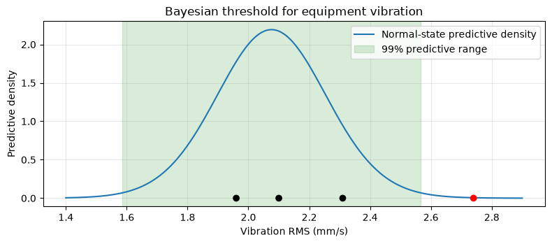
Regarding the vibration RMS values of assembly equipment, the following observation distribution is created from the normal-state data, and inspections are determined based on threshold values that include uncertainty in normal conditions, rather than fixed values.

Approach to Analysis and Modeling

The normal value is taken as the normal distribution, and the post-post prediction when the mean and variance are unknown is the $t$ distribution of the Student. If the bilateral postmortem prediction probability of the new observation $x_\mathrm{new}$ is low, it is an anomaly candidate.

Check with Python

normal_vibration=rng.normal(2.05,.16,40)
new_vibration=np.array([2.10,2.31,2.74,1.96])
n=len(normal_vibration); mean=normal_vibration.mean(); s=normal_vibration.std(ddof=1)
pred_scale=s*np.sqrt(1+1/n); dist=stats.t(df=n-1,loc=mean,scale=pred_scale)
lower,upper=dist.ppf([.005,.995])
tail=2*np.minimum(dist.cdf(new_vibration),1-dist.cdf(new_vibration))
result_089=pd.DataFrame({"vibration":new_vibration,"two_sided_predictive_p":tail,"alert":tail<.01})
display(result_089.round(5)); print(f"99% posterior predictive interval: [{lower:.3f}, {upper:.3f}]")
fig,ax=plt.subplots(figsize=(8,3.6)); x=np.linspace(1.4,2.9,500); ax.plot(x,dist.pdf(x),label="Normal-state predictive density")
ax.axvspan(lower,upper,alpha=.15,color="green",label="99% predictive range"); ax.scatter(new_vibration,np.zeros_like(new_vibration),c=np.where(tail<.01,"red","black"),zorder=3)
ax.set_title("Bayesian threshold for equipment vibration"); ax.set_xlabel("Vibration RMS (mm/s)"); ax.set_ylabel("Predictive density")
ax.grid(alpha=.3); ax.legend(); plt.tight_layout(); plt.show()

	vibration	two_sided_predictive_p	alert
0	2.10	8.953e-01	False
1	2.31	2.033e-01	False
2	2.74	7.200e-04	True
3	1.96	5.247e-01	False

99% posterior predictive interval: [1.586, 2.566]

Reading the results

Red spots are unlikely to occur on normal models and are recommended for inspection. However, rather than the probability of abnormalities themselves, we look at how rare it is if it were normal. Stop decisions include the probability of failure beforehand, missed or false alarm costs, multiple sensors, and the number of consecutive incidents.

No.090: Compile Bayesian Analysis Results into Business Reports

Meaning in Practice

Instead of listing model coefficients, it consolidates decision-making, probability, amount, recommended action, and reservations into a single sheet. The goal is to have decision-making rules that can be reproducible to anyone other than the analyst.

Approach to Analysis and Modeling

In the report, (1) questions, (2) data periods, (3) prior distributions, (4) post-event predictions, (5) decision criteria, and (6) sensitivity and limitations are separated. Instead of automatically determining results based solely on probability, both the loss function and business constraints are recorded together.

Check with Python

report=pd.DataFrame([
 ["Next-month capacity",f"P95 demand = {np.quantile(demand_next,.95):.0f} units","Check material/capacity at P95","Demand model uses recent 6 months"],
 ["Sales budget",f"P(>= JPY {budget:.0f}M) = {np.mean(sales_next>=budget):.1%}","Prepare P05 cash scenario","Price and quantity simulated"],
 ["Campaign",f"P(lift > 5pt) = {np.mean(lift>.05):.1%}","Compare expected margin with cost","Observational follow-up may differ"],
 ["Equipment alert",f"{result_089.alert.sum()} of {len(result_089)} readings","Inspect alert readings","Confirm with other sensors"]],
 columns=["decision","evidence","recommended_action","caveat"])
display(report)

	decision	evidence	recommended_action	caveat
0	Next-month capacity	P95 demand = 137 units	Check material/capacity at P95	Demand model uses recent 6 months
1	Sales budget	P(>= JPY 16M) = 26.7%	Prepare P05 cash scenario	Price and quantity simulated
2	Campaign	P(lift > 5pt) = 76.0%	Compare expected margin with cost	Observational follow-up may differ
3	Equipment alert	1 of 4 readings	Inspect alert readings	Confirm with other sensors

Reading the results

By listing “evidence,” “action,” and “reservation” in the same table, you prevent probability from going on a whim. Update dates, code versions, data extraction conditions, and approvers are also attached to the production report, and forecasts and results are reconciled the following month.

Practical Implications Seen Through Target Exercise

The value of Bayesian analysis lies not in advanced distribution names, but in the ability to explicitly use past knowledge even when information is scarce, continuously update with new data, and directly calculate the probabilities necessary for decision-making. Rather than managing demand, customers, and quality with separate point estimates, it is easier to align cross-departmental judgment criteria by summarizing forecast distributions based on “which losses you want to avoid.”

What is necessary for practical implementation

1. Decision Making and Defining Loss: Agree on costs for out-of-stock, surplus, false alarms, and missed items
2. Verification of the Data Generation Process: Record missed measurements, discontinuations, price revisions, and selection of policy targets
3. Review of the preliminary distribution: Leave evidence and sensitivity analysis to prevent convenient adjustments
4. validation: Regularly conduct post-forecast checks, time-series backtests, and calibrations
5. Operations Design: Determine update frequency, responsible persons, exception handling, and conditions for model stoppage

Conclusion

In No.081 to No.090, we focused on conjugate models and simulations to represent the uncertainties in demand, sales, policies, customers, and equipment in manufacturing as probabilities. The next step is to define your company’s unique losses and constraints, evaluating them not only by forecast accuracy but also by post-decision benefits, service levels, and safety.

Consultations for Corporations

When introducing demand forecasting, inventory and production planning, promotional effect verification, and predictive maintenance, it is necessary to design not only model creation but also data definition, on-site decision-making rules, and operations and training in an integrated manner. At Mathematical Laboratory, we support PoC design, analytical infrastructure, in-house training, and implementation in decision-making processes.

📩 Contact Us: surikobo.co.jp/contact
Please feel free to consult us first.