100 Exercises / Bayesian statistics / Bayesian Statistics 100 Exercises for Data Analysis

Bayesian Estimation of Manufacturing Non-Performing Rate | Applying Credit Bands, Exceeding Standards Probability, and Next Lot Forecast with Python

2020-09-16

Determining Process Improvements from Small Amounts of Inspection Data—Practical Bayesian Estimation and Forecasting

In manufacturing sites, simply reporting the defect rate as a single value does not make it difficult to determine shipment feasibility or investment in improvements. In this article, we use the Current LineA and Improvement Candidate LineB sampling inspections at a fictional precision parts factory as a subject, and implement the process of “turning estimated uncertainty into decision-making” through No.041 to No.050.

The questions addressed include the current defect rate, whether it could exceed control standards, whether line B is truly improving, and how many defects are expected in the next lot. External data is not used; instead, fictional data generated by fixed seeds is used.

[!NOTE] This material is a notebook previously used by Surikoubo (or personally by the representative, Kazuyama), and has been reconstructed, edited, and published with the company’s permission. All data listed is fictional and has no relation whatsoever to real companies, factories, or figures.

Introduction: Practical Challenges in Manufacturing Covered in This Article

At one factory, non-standard critical dimensions are defined as “defects” and are conducting spot checks on a separate line. The management guideline is a defect rate of 2%. However, if the number of tests is only a few hundred, the error rate can fluctuate even by chance. Judging solely by “1.7% is no problem” or “2.2% is why stop” leads to both overreaction and missed detection.

In this article, we set the defect probability as an unknown parameter $p$ and calculate the post-event distribution from the pre-distribution and test results. On top of that, we cover everything from process status explanation, line comparison, next lot prediction, model verification, to report creation.

Common situations on site

The daily report only lists ‘number of tests, number of defects, and defect rate,’ and does not indicate uncertainty.
Interpreting the difference in rates before and after improvement as the effect of improvement
You cannot discuss probability exceeding management standards alone
Estimates based on historical data are often confused with variations in future lots.
Report only results without checking for discrepancies between model predictions and actual measurements.

Why is this issue so difficult to judge?

If the number of defects $x$ is the binomial distribution $x\sim\mathrm{Binomial}(n,p)$ among $n$ , even with the same true defect rate, the $x$ changes with each inspection. Also, the uncertainty of the estimated $p$ and the variation in chance occurring in the next lot are two different things. Bayesian statistics represent the former as posterior distributions, and the combined result as the posterior prediction distribution.

Overview of Exercise covered this time

No.	Theme	Questions Answered in Practice
041	Post-event average	Here are some representative defect rate values:
042	median post hoc	What is the value that halves the post-event probability?
043	MAP Estimates	What is the defect rate with the highest density?
044	credit range	Where is the most plausible range for defect rates?
045	Probability of exceeding threshold	What is the probability that the defect rate exceeds the 2% management standard?
046	2. Difference in probability	What is the probability and extent of improvement for line B over A?
047	Postmortem Distribution	How to predict the number of defects in the next lot
048	Predicted Section	What is the realistic range for defective numbers in the next lot?
049	Forecast Check	Are there any major discrepancies between the model and actual measurements?
050	Report	How to communicate results to decision-makers

Preparing the Python environment

Only NumPy, pandas, SciPy, and matplotlib are used. Create a random number generator and fix the seed so that the result is the same when you run it again.

import sys
import numpy as np
import pandas as pd
import scipy
from scipy.stats import beta, betabinom
import matplotlib
import matplotlib.pyplot as plt
from IPython.display import display, Markdown

SEED = 20250715
rng = np.random.default_rng(SEED)
plt.rcParams["figure.figsize"] = (8, 4.5)
plt.rcParams["axes.unicode_minus"] = False
plot_label = {"A(Current)": "Line A (current)", "B(Improvement candidate)": "Line B (candidate)"}

print(f"Python     : {sys.version.split()[0]}")
print(f"NumPy      : {np.__version__}")
print(f"pandas     : {pd.__version__}")
print(f"SciPy      : {scipy.__version__}")
print(f"matplotlib : {matplotlib.__version__}")

Python     : 3.13.1
NumPy      : 2.5.1
pandas     : 3.0.3
SciPy      : 1.18.0
matplotlib : 3.11.0

Creation of Fictional Data

For each line, let’s say you remove 20 items per day for 25 days. As training data, fixed daily inspection and defect counts are generated in Python. Line A is a candidate based on current conditions, and Line B is a candidate with revised equipment conditions. The data here is a hypothetical value for explanatory purposes.

days = pd.date_range("2025-06-02", periods=25, freq="B")
records = []
for line, true_rate in {"A(Current)": 0.024, "B(Improvement candidate)": 0.014}.items():
    defects = rng.binomial(20, true_rate, size=len(days))
    for day, x in zip(days, defects):
        records.append({"date": day, "line": line, "inspected": 20, "defects": int(x)})

inspection = pd.DataFrame(records)
summary = (inspection.groupby("line", as_index=False)
           .agg(inspected=("inspected", "sum"), defects=("defects", "sum")))
summary["observed_rate"] = summary["defects"] / summary["inspected"]
display(inspection.head(8))
display(summary.style.format({"observed_rate": "{:.2%}"}))

	date	line	inspected	defects
0	2025-06-02	A(Current)	20	0
1	2025-06-03	A(Current)	20	0
2	2025-06-04	A(Current)	20	0
3	2025-06-05	A(Current)	20	0
4	2025-06-06	A(Current)	20	2
5	2025-06-09	A(Current)	20	1
6	2025-06-10	A(Current)	20	0
7	2025-06-11	A(Current)	20	0

	line	inspected	defects	observed_rate
0	A(Current)	500	10	2.00%
1	B(Improvement candidate)	500	8	1.60%

daily = inspection.pivot(index="date", columns="line", values="defects")
ax = daily.rename(columns=plot_label).plot(marker="o", linewidth=1.2)
ax.set_title("Daily defects in 20 inspected units")
ax.set_xlabel("Inspection date")
ax.set_ylabel("Number of defects")
ax.grid(True, alpha=0.3)
plt.tight_layout()
plt.show()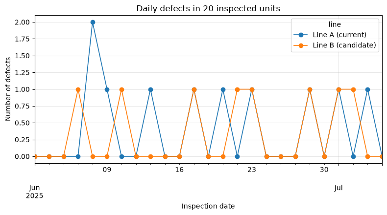

png

Common Model Settings

Regarding past similar processes, the defect rate is mainly about 2%, but we do not strongly judge it with $p\sim\mathrm{Beta}(2,98)$ . This is about the amount of information you can virtually see 100 items and find that 2 were defective. When $x$ defects are observed with $n$ tests, due to conjugation,

$p\mid x,n\sim\mathrm{Beta}(\alpha+x,\;\beta+n-x)$

That’s how it works. In practice, we agree on pre-distribution with quality assurance and production technology, and also conduct sensitivity analysis using multiple pre-distributions.

prior_a, prior_b = 2, 98
post = summary.copy()
post["alpha"] = prior_a + post["defects"]
post["beta"] = prior_b + post["inspected"] - post["defects"]
post = post.set_index("line")
display(post)

	inspected	defects	observed_rate	alpha	beta
line
A(Current)	500	10	0.020	12	588
B(Improvement candidate)	500	8	0.016	10	590

No.041: Calculating Post-Histories Averages

Meaning in Practice

The posterior mean is a Bayesian estimate when the square error is considered a loss. It is useful when a single representative value is needed for daily reports or KPIs, but it is also necessary to list the distribution range. In the Beta distribution, it is $E[p\mid x]=\alpha'/(\alpha'+\beta')$ .

Approach to Analysis and Modeling

Post-event or post-event distribution is linked to on-site management standards, scope of improvement, and future number of units. The goal is not to calculate estimates themselves, but to clarify which losses to avoid and which additional information will change the decision.

Check with Python

post["posterior_mean"] = post["alpha"] / (post["alpha"] + post["beta"])
display(post[["observed_rate", "posterior_mean"]].style.format("{:.3%}"))

	observed_rate	posterior_mean
line
A(Current)	2.000%	2.000%
B(Improvement candidate)	1.600%	1.667%

Reading the results

Post-event averages are positioned between the observed rate and the pre-event average. The smaller the sample size, the greater the influence of prior information, which helps suppress overreaction to random swings. However, shipment approval is not determined solely by the average; instead, the sections and probabilities for No.044 and 045 are checked.

No.042: Calculating the Post-Posterior Median

Meaning in Practice

The posterior median $m$ meets $P(p\le m\mid x)=0.5$ . In a distorted distribution, unlike the mean, the representative value is represented by the absolute error loss. It is worth comparing with indicators that tend to distort near zero, such as low defect rates.

Approach to Analysis and Modeling

Check with Python

post["posterior_median"] = [beta.median(r.alpha, r.beta) for r in post.itertuples()]
display(post[["posterior_mean", "posterior_median"]].style.format("{:.3%}"))

	posterior_mean	posterior_median
line
A(Current)	2.000%	1.947%
B(Improvement candidate)	1.667%	1.613%

Reading the results

Although the difference between the average and median is small, it is not identical. When the rate is low and the number of defects is small, the right end of the distribution may be longer, and the average may be slightly above the median. Clearly state the definition of representative values in the report.

No.043: Calculating MAP Estimates

Meaning in Practice

MAP (maximum a posteriori) is the value where post-mortem density is maximized. When the Beta distribution is $\alpha',\beta'>1$ , it is $(\alpha'-1)/(\alpha'+\beta'-2)$ . It shows the most “likely point,” but the probability of a continuous point itself is zero and is not a substitute for the interval.

Approach to Analysis and Modeling

Check with Python

post["map"] = (post["alpha"] - 1) / (post["alpha"] + post["beta"] - 2)
display(post[["posterior_mean", "posterior_median", "map"]].style.format("{:.3%}"))

	posterior_mean	posterior_median	map
line
A(Current)	2.000%	1.947%	1.839%
B(Improvement candidate)	1.667%	1.613%	1.505%

Reading the results

The closeness of the mean, median, and MAP indicates that the estimate is not extremely skewed. However, in decision-making, estimates should be chosen based on the loss function used, and “MAP is not always correct.”

No.044: Calculating the Credit Bracket

Meaning in Practice

The 95% equivalent-tail credit interval is constructed at the lower 2.5% point and the upper 97.5% point of the posterior distribution. The Bayesian credit range can be interpreted as a 95% post-event probability that $p$ falls within this range, based on the model and data.

Approach to Analysis and Modeling

Check with Python

post["ci_low"] = [beta.ppf(0.025, r.alpha, r.beta) for r in post.itertuples()]
post["ci_high"] = [beta.ppf(0.975, r.alpha, r.beta) for r in post.itertuples()]
display(post[["posterior_mean", "ci_low", "ci_high"]].style.format("{:.3%}"))

plot_df = post.reset_index()
err = np.vstack([plot_df.posterior_mean - plot_df.ci_low,
                 plot_df.ci_high - plot_df.posterior_mean])
fig, ax = plt.subplots()
ax.errorbar(plot_df["line"].map(plot_label), plot_df.posterior_mean, yerr=err,
            fmt="o", capsize=6, color="tab:blue")
ax.axhline(0.02, color="tab:red", linestyle="--", label="Control threshold: 2%")
ax.set_title("Posterior mean and 95% credible interval")
ax.set_xlabel("Production line")
ax.set_ylabel("Defect probability")
ax.grid(True, alpha=0.3)
ax.legend()
plt.tight_layout()
plt.show()

	posterior_mean	ci_low	ci_high
line
A(Current)	2.000%	1.039%	3.262%
B(Improvement candidate)	1.667%	0.803%	2.833%

png

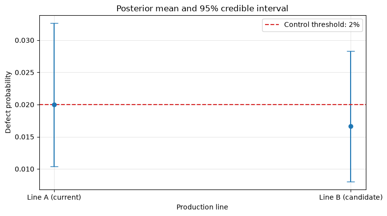
Reading the results

Just because the sections overlap doesn’t mean there is “no difference.” Also, if the section of Line A crosses the standard, a point estimate below 2% does not guarantee safety. This situation is highly worthwhile for additional examinations.

No.045: Calculating the probability that parameters exceed a constant value

Meaning in Practice

If we set the management standard to $p_{limit}=2\%$ , the probability of exceeding is $P(p>p_{limit}\mid x)=1-F_{Beta}(p_{limit})$ . You can present the probability of ‘exceeding the standard or not’ to the quality meeting. Actual shutdown standards are designed in conjunction with losses, regulations, and customer requirements.

Approach to Analysis and Modeling

Check with Python

limit = 0.02
post["prob_over_2pct"] = [beta.sf(limit, r.alpha, r.beta) for r in post.itertuples()]
display(post[["posterior_mean", "prob_over_2pct"]].style.format("{:.2%}"))

xgrid = np.linspace(0, 0.07, 600)
fig, ax = plt.subplots()
for line, row in post.iterrows():
    density = beta.pdf(xgrid, row.alpha, row.beta)
    ax.plot(xgrid, density, label=plot_label[line])
    ax.fill_between(xgrid, density, where=xgrid > limit, alpha=0.18)
ax.axvline(limit, color="black", linestyle="--", label="Threshold: 2%")
ax.set_title("Posterior distributions and threshold exceedance")
ax.set_xlabel("Defect probability")
ax.set_ylabel("Posterior density")
ax.grid(True, alpha=0.3)
ax.legend()
plt.tight_layout()
plt.show()

	posterior_mean	prob_over_2pct
line
A(Current)	2.00%	46.28%
B(Improvement candidate)	1.67%	24.15%

png

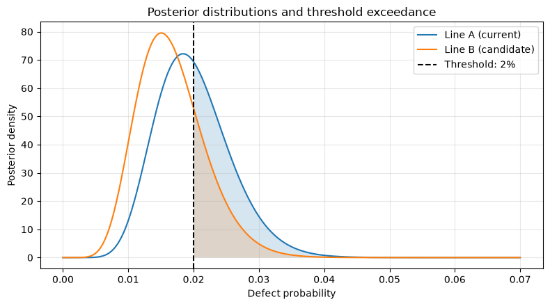
Reading the results

The excess probability is the posterior area to the right of the baseline. This can be linked to rules like “80% or higher, process check,” or “95% or more, pause,” but thresholds quantify the costs of false stops and outflows.

No.046: Calculating the posterior distribution of the difference between two probabilities

Meaning in Practice

Samples $p_A,p_B$ from independent posterior distributions and calculates the $\Delta=p_A-p_B$ of improvement. $P(\Delta>0)$ is the probability that B has a lower defect rate than A, and $P(\Delta>0.005)$ is the probability of improving by 0.5 points or more.

Approach to Analysis and Modeling

Check with Python

draws = 200_000
pa = rng.beta(post.loc["A(Current)", "alpha"], post.loc["A(Current)", "beta"], draws)
pb = rng.beta(post.loc["B(Improvement candidate)", "alpha"], post.loc["B(Improvement candidate)", "beta"], draws)
delta = pa - pb
comparison = pd.Series({
    "mean_improvement": delta.mean(),
    "prob_B_better": np.mean(delta > 0),
    "prob_improvement_over_0.5pt": np.mean(delta > 0.005),
    "ci_low": np.quantile(delta, 0.025),
    "ci_high": np.quantile(delta, 0.975),
})
display(comparison.to_frame("value").style.format("{:.2%}"))

fig, ax = plt.subplots()
ax.hist(delta, bins=80, density=True, alpha=0.75, color="tab:green")
ax.axvline(0, color="black", linestyle="--", label="No difference")
ax.axvline(0.005, color="tab:red", linestyle=":", label="0.5 pt improvement")
ax.set_title("Posterior distribution of improvement (pA - pB)")
ax.set_xlabel("Reduction in defect probability")
ax.set_ylabel("Density")
ax.grid(True, alpha=0.3)
ax.legend()
plt.tight_layout()
plt.show()

	value
mean_improvement	0.34%
prob_B_better	67.09%
prob_improvement_over_0.5pt	41.07%
ci_low	-1.18%
ci_high	1.88%

png

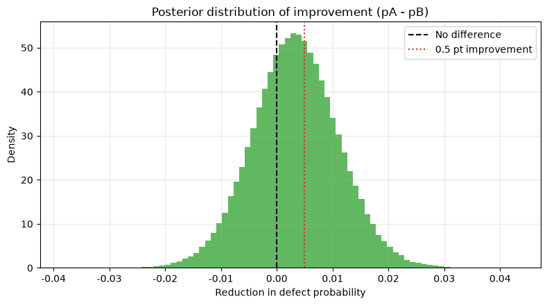
Reading the results

Not only is the observation rate of B low, but it can also be shown separately as the probability that B is superior and the probability that the improvement exceeds practical significance. Even if statistical advantage is high, if the improvement is small, the modification costs may not be recovered.

No.047: Creating Post-Prediction Distributions

Meaning in Practice

The next lot $m$ defective numbers $Y$ follows a beta binomial distribution that integrates the uncertainty of the $p$ . $Y\mid x\sim\mathrm{BetaBinomial}(m,\alpha',\beta')$ is this. Here, we predict the next 200 lots for each line.

Approach to Analysis and Modeling

Check with Python

future_n = 200
k = np.arange(future_n + 1)
predictive = {}
for line, row in post.iterrows():
    predictive[line] = betabinom.pmf(k, future_n, row.alpha, row.beta)

fig, ax = plt.subplots()
for line, pmf in predictive.items():
    ax.plot(k[:18], pmf[:18], marker="o", label=plot_label[line])
ax.set_title("Posterior predictive distribution for next 200 units")
ax.set_xlabel("Number of defects in next lot")
ax.set_ylabel("Predictive probability")
ax.grid(True, alpha=0.3)
ax.legend()
plt.tight_layout()
plt.show()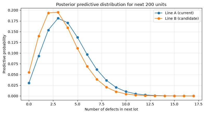

png

Reading the results

The predicted distribution directly represents how many defects may occur in the next lot. For tasks planned by “quantity,” such as reserved space, re-inspection man-hours, and replacement inventory, the post-forecast distribution is more suitable than the credit range of the parameter.

No.048: Calculating Forecast Intervals

Meaning in Practice

The 95% prediction range is the range where defects in the next lot are expected to occur. This is not a credit range for the non-performing rate parameter, but also includes binomial fluctuations observed in the future, so it is relatively broad.

Approach to Analysis and Modeling

Check with Python

pred_rows = []
for line, row in post.iterrows():
    dist = betabinom(future_n, row.alpha, row.beta)
    pred_rows.append({
        "line": line,
        "expected_defects": dist.mean(),
        "prediction_low": int(dist.ppf(0.025)),
        "prediction_high": int(dist.ppf(0.975)),
        "prob_5_or_more": dist.sf(4),
    })
pred_summary = pd.DataFrame(pred_rows).set_index("line")
display(pred_summary.style.format({"expected_defects": "{:.2f}", "prob_5_or_more": "{:.1%}"}))

	expected_defects	prediction_low	prediction_high	prob_5_or_more
line
A(Current)	4.00	0	9	37.0%
B(Improvement candidate)	3.33	0	8	25.8%

Reading the results

By looking not only at the expected number of defects but also at the upper predicted points, you can design with more margins in personnel and re-inspection capacity. Simply saying, ‘Average 3 pieces, so only prepare 3 units’ cannot handle the upside fluctuations that normally occur.

No.049: Comparing Observations and Post-Prediction Distributions

Meaning in Practice

We check with post-prediction checks to see if the model can reproduce the features of field data. This time, we reproduce the number of defects among 20 items per day and compare the “number of days with zero defects” with the “maximum number of defects per day.” If measurements are taken at extreme locations, factors such as daily fluctuations, lot differences, and equipment condition can be added to the model.

Approach to Analysis and Modeling

Check with Python

n_rep = 50_000
ppc_rows = []
fig, axes = plt.subplots(1, 2, figsize=(11, 4.2))
for ax, (line, row) in zip(axes, post.iterrows()):
    p_rep = rng.beta(row.alpha, row.beta, size=(n_rep, 1))
    replicated = rng.binomial(20, p_rep, size=(n_rep, 25))
    rep_zero_days = (replicated == 0).sum(axis=1)
    observed = daily[line].to_numpy()
    obs_zero_days = int((observed == 0).sum())
    ppc_rows.append({
        "line": line,
        "observed_zero_days": obs_zero_days,
        "predictive_mean_zero_days": rep_zero_days.mean(),
        "two_sided_tail_area": 2 * min(np.mean(rep_zero_days <= obs_zero_days),
                                         np.mean(rep_zero_days >= obs_zero_days)),
    })
    ax.hist(rep_zero_days, bins=np.arange(-0.5, 26.5), alpha=0.75)
    ax.axvline(obs_zero_days, color="tab:red", linestyle="--", label="Observed")
    ax.set_title(f"PPC: {plot_label[line]}")
    ax.set_xlabel("Zero-defect days out of 25")
    ax.set_ylabel("Simulation frequency")
    ax.grid(True, alpha=0.3)
    ax.legend()
plt.tight_layout()
plt.show()
ppc = pd.DataFrame(ppc_rows).set_index("line")
display(ppc.style.format({"predictive_mean_zero_days": "{:.1f}", "two_sided_tail_area": "{:.3f}"}))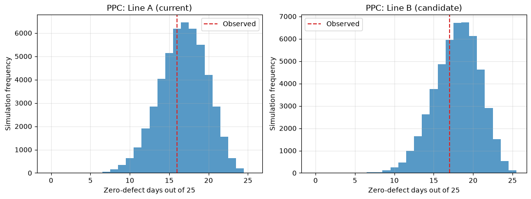

png

	observed_zero_days	predictive_mean_zero_days	two_sided_tail_area
line
A(Current)	16	16.8	0.897
B(Improvement candidate)	17	18.0	0.829

Reading the results

Check whether the red line is at the extreme end of the predicted distribution. This check does not prove the model is correct. If there is inconsistency, do not stick to a simple binomial model, but consider daily and equipment hierarchical structures and overdispersion.

No.050: Compiling Bayesian Estimation Results as a Report

Meaning in Practice

In the decision maker report, the method name indicates “conclusion, uncertainty, recommended action, assumptions” first. Below, we automatically generate a routine summary from the calculated values. A design that allows pre-rounding data for audit purposes is also desirable.

Approach to Analysis and Modeling

Check with Python

report = pd.DataFrame({
    "indicator": ["Post-event average defect rate", "95%credit range", "2%excess probability", "Next200Individual Expected Defects", "Next200individual95%Predicted Section"],
    "A(Current)": [
        f"{post.loc['A(Current)','posterior_mean']:.2%}",
        f"{post.loc['A(Current)','ci_low']:.2%}–{post.loc['A(Current)','ci_high']:.2%}",
        f"{post.loc['A(Current)','prob_over_2pct']:.1%}",
        f"{pred_summary.loc['A(Current)','expected_defects']:.1f}units",
        f"{pred_summary.loc['A(Current)','prediction_low']}–{pred_summary.loc['A(Current)','prediction_high']}units",
    ],
    "B(Improvement candidate)": [
        f"{post.loc['B(Improvement candidate)','posterior_mean']:.2%}",
        f"{post.loc['B(Improvement candidate)','ci_low']:.2%}–{post.loc['B(Improvement candidate)','ci_high']:.2%}",
        f"{post.loc['B(Improvement candidate)','prob_over_2pct']:.1%}",
        f"{pred_summary.loc['B(Improvement candidate)','expected_defects']:.1f}units",
        f"{pred_summary.loc['B(Improvement candidate)','prediction_low']}–{pred_summary.loc['B(Improvement candidate)','prediction_high']}units",
    ],
}).set_index("indicator")
display(report)

recommendation = f"""### Summary for Quality Meetings (Fictitious Data)

- LineBbutAPost-mortem probability, which is a lower defect rate, is **{np.mean(delta > 0):.1%}**。
- The range of improvement0.5The probability of exceeding the points is **{np.mean(delta > 0.005):.1%}**。
- However, since the estimated range remains, additional verification is conducted with the same product and inspection conditions before switching.
- In additional verification, hiring criteria are pre-fixed based on customer churn costs and stoppage costs.
"""
display(Markdown(recommendation))

	A(Current)	B(Improvement candidate)
indicator
Post-event average defect rate	2.00%	1.67%
95%credit range	1.04%–3.26%	0.80%–2.83%
2%excess probability	46.3%	24.2%
Next200Individual Expected Defects	4.0units	3.3units
Next200individual95%Predicted Section	0–9units	0–8units

Summary for Quality Meetings (Fictitious Data)

The posterior probability that line B has a lower defect rate than A is 67.1%.
The probability of improvement exceeding 0.5 points is 41.1%.
However, since the estimated range remains, additional verification is conducted with the same product and inspection conditions before switching.
In additional verification, hiring criteria are pre-fixed based on customer churn costs and stoppage costs.

Reading the results

A good report not only lists point estimation but also probability, intervals, operational thresholds, and next actions in the same table. Furthermore, this conclusion assumes binomial models, prior distribution, inspection independence, and inspection accuracy, and requires verification before applying them to actual processes.

Practical Implications Seen Through Target Exercise

Representative values, intervals, and excess probabilities have different roles: KPIs should focus on post-mortem averages, explanations should focus on credit ranges, and behavioral criteria should focus on threshold exceeding probabilities.
Distinguishing the probability of a difference from its magnitude: The probability that Line B is superior alone does not determine the economic rationality of capital investment. Define the minimum practical difference.
Use predictive distributions for future planning: Instead of parameter estimation, we design re-inspection personnel, inventory, and delivery risks based on the number of defective items in the next lot.
Predictive checks are the entry point to operations.: If daily variations cannot be reproduced, explanatory variables and hierarchical structures such as variety, equipment, material lots, and work teams are examined.
Converting probability into action requires costs: Decision-making rules only become after defining losses from outflows, stoppages, reinspections, switchings, and delivery delays.

What is necessary for practical implementation

Standardize defect definitions, inspection units, populations, and measurement systems.
Define the target periods and similar processes for past data, and record the basis for prior distribution.
Confirm the independence of inspections, product composition, and heterogeneity by equipment, work teams, and material lots
Conduct sensitivity analysis with altered pre-distribution and external verification over time series
Decide what to do if the probability of exceeding the standard is greater than what is the risk, including losses and those responsible.
Incorporate data updates, recalculations, approvals, version management, and audit logs into your workflow
If errors by inspectors or measuring instruments cannot be ignored, they are included in the observation model.

Conclusion

In No.041–050, we used a Beta-Binomial model to implement representative defect rates, credit intervals, probability of exceeding the standard, line differences, next lot prediction, forecast checks, and reporting. The value of Bayesian estimates is not in asserting that the defect rate is 1.8%, but in being able to make a common language about “how uncertain and which actions are reasonable.”

This example is a simplified starting point. In practice, by incorporating hierarchical factors such as day, equipment, variable, and material lots, time changes, inspection errors, and decision-making costs, we develop a system that can withstand on-site judgments.

Consultations for Corporations

At Suri Kobo, we support everything from Bayesian model design targeting manufacturing quality data, PoC, integration with existing KPIs, on-site training, to implementing regular reports and dashboards. You can consult with us from stages such as small data volumes, large differences between processes, or wanting to make threshold judgments explainable.

📩 Contact Us: surikobo.co.jp/contact Please feel free to consult us first.

Bayesian Estimation of Manufacturing Non-Performing Rate | Applying Credit Bands, Exceeding Standards Probability, and Next Lot Forecast with Python

Determining Process Improvements from Small Amounts of Inspection Data—Practical Bayesian Estimation and Forecasting

Introduction: Practical Challenges in Manufacturing Covered in This Article

Common situations on site

Why is this issue so difficult to judge?

Overview of Exercise covered this time

Preparing the Python environment

Creation of Fictional Data

Common Model Settings

No.041: Calculating Post-Histories Averages

Meaning in Practice

Approach to Analysis and Modeling

Check with Python

Reading the results

No.042: Calculating the Post-Posterior Median

Meaning in Practice

Approach to Analysis and Modeling

Check with Python

Reading the results

No.043: Calculating MAP Estimates

Meaning in Practice

Approach to Analysis and Modeling

Check with Python

Reading the results

No.044: Calculating the Credit Bracket

Meaning in Practice

Approach to Analysis and Modeling

Check with Python

Reading the results

No.045: Calculating the probability that parameters exceed a constant value

Meaning in Practice

Approach to Analysis and Modeling

Check with Python

Reading the results

No.046: Calculating the posterior distribution of the difference between two probabilities

Meaning in Practice

Approach to Analysis and Modeling

Check with Python

Reading the results

No.047: Creating Post-Prediction Distributions

Meaning in Practice

Approach to Analysis and Modeling

Check with Python

Reading the results

No.048: Calculating Forecast Intervals

Meaning in Practice

Approach to Analysis and Modeling

Check with Python

Reading the results

No.049: Comparing Observations and Post-Prediction Distributions

Meaning in Practice

Approach to Analysis and Modeling

Check with Python

Reading the results

No.050: Compiling Bayesian Estimation Results as a Report

Meaning in Practice

Approach to Analysis and Modeling

Check with Python

Summary for Quality Meetings (Fictitious Data)

Reading the results

Practical Implications Seen Through Target Exercise

What is necessary for practical implementation

Conclusion

Consultations for Corporations

Related Posts

Introduction to Bayesian Decision-Making in Manufacturing | Explaining Expected Loss, Inventory Optimization, and Practical Implementation in Python

Introduction to Bayesian Statistics in Manufacturing | Practice Demand Forecasting, Sales Promotion, and Anomaly Detection with Python

Stable Estimation of Manufacturing Line Defect Rates Using Hierarchical Bayes | Utilizing Small Data for Decision-Making

Introduction to Bayesian Regression in Manufacturing | Predicting Order Amount, Order Probability, and Number of Inquiries Using Python

Introduction to Bayesian A/B Testing in Manufacturing | Comparing Inspection Conditions by Probability and Expected Returns