Selecting inspection conditions based on business value rather than “win rate”: Practical Bayesian A/B testing in manufacturing

In manufacturing sites, when changing thresholds for image inspection, work standards, or equipment conditions, issues arise such as “It looks like an improvement, but is it just a coincidence?” “When to stop testing,” and “Can it be adopted considering not only quality but also cost?” In this article, we consistently cover everything from A/B test design to multi-proposal comparisons and decision-making rules, using a fictional image inspection process as the subject, using Bayesian statistics.

The target is No.051〜No.060(Chapter6Chapter: BayesA/BTest). A is the current condition, B is the new condition, and the percentage of good products that pass correctly is treated as CVR (here, the ‘positive judgment rate’).

[!NOTE] This material is a notebook previously used by Surikoubo (or personally by the representative, Kazuyama), and has been reconstructed, edited, and published with the company’s permission. All data listed is fictional and has no relation whatsoever to real companies, factories, or figures.

1. Introduction: Practical Challenges in Manufacturing Covered in This Article

In the image inspection process, there is an increase in ‘over-detection,’ where good products are discarded as defective. The technical department proposed new condition B, but switching incurred revalidation costs. The question in this paper is not simply whether B has a high correct observation rate, but Including the costs of uncertainty and misjudgmentBShould we adopt them?.

2. Common Situations on Site

• Before the number of A and B exams is aligned, conclusions are reached at the daily meeting.
• Judging only by the magnitude of the observation rate, with uncertainty about the extent of improvement not being shared.
• There are biases in variety, shift, and equipment, undermining comparability
• Only probability criteria like “95% hire you” will stand on their own.
• Sometimes improvements are too small to cover the replacement costs.

3. Why is this issue difficult to judge?

The observation rate for finite samples fluctuates. Also, “statistically there seems to be a difference” and “sufficient business improvement” are different things. Operations that adjust downtime based on data, simultaneous comparison of multiple options, and asymmetry in implementation losses also make decision-making difficult. Bayesian A/B tests represent unknown correct judgment rates as distributions and can be converted into probabilities, expected improvements, and expected losses that can be directly used in decision-making.

4. The overall picture of exercise covered this time

No.	Theme	Questions Answered On-Site
051	Purpose	What to define as improvement
052	Comparison	What is the difference between frequentism and Bayesianism?
053	Beta distribution	How to Express the Unknown Rate of A/B
054	Post-event distribution	How to update experimental data
055	superior probability	There are several odds that B is better than A.
056	Distribution of differences	How far can the improvement range be affected?
057	Expected improvement	How effective is it on average
058	minority specimen	How to suppress early decision-making
059	A/B/n	How to choose from multiple candidates
060	Rules of Judgment	How to integrate quality and cost

5. Preparing the Python environment

Only NumPy, pandas, SciPy, and matplotlib are used. The random number generator is fixed so that rerunning it yields the same result.

import platform
import numpy as np
import pandas as pd
import matplotlib
import matplotlib.pyplot as plt
import scipy
from scipy.stats import beta, fisher_exact

rng = np.random.default_rng(20250715)
plt.rcParams["figure.figsize"] = (8, 4.5)
plt.rcParams["axes.unicode_minus"] = False

print("Python     :", platform.python_version())
print("NumPy      :", np.__version__)
print("pandas     :", pd.__version__)
print("SciPy      :", scipy.__version__)
print("matplotlib :", matplotlib.__version__)

Python     : 3.13.1
NumPy      : 2.5.1
pandas     : 3.0.3
SciPy      : 1.18.0
matplotlib : 3.11.0

6. Creation of Fictional Data

Assuming random assignments for the same type and equipment group, the number of inspections and positive judgments for A/B is generated. In actual implementation, it is necessary to stratify varieties, equipment, and shifts, and fix allocation ratios and exclusion criteria before testing.

true_rates = {"A(Current)": 0.930, "B(New Conditions)": 0.947}
n_per_arm = 800
rows = []
for variant, true_rate in true_rates.items():
    correct = rng.binomial(n_per_arm, true_rate)
    rows.append({"variant": variant, "inspected": n_per_arm,
                 "correct": correct, "incorrect": n_per_arm - correct})

ab = pd.DataFrame(rows)
ab["observed_rate"] = ab["correct"] / ab["inspected"]
ab.style.format({"observed_rate": "{:.2%}"})

	variant	inspected	correct	incorrect	observed_rate
0	A(Current)	800	750	50	93.75%
1	B(New Conditions)	800	763	37	95.38%

No.051: Organize the Purpose of A/B Testing

Meaning in Practice

The purpose of the test is not that “the number B is greater than A.” Agree on the main KPIs, guardrails, minimum practical difference, target population, and evaluation period in advance, and convert them into questions that will lead to post-adoption profit and loss. In this example, the main KPI is the correct judgment rate for good products, the minimum practical difference is 0.5 points, and the guardrail is used as processing time and missed rate.

Approach to Analysis and Modeling

Let the correct judgment per observation unit be $Y_i\in\{0,1\}$, and the probability of correct judgment for condition $j$ be $p_j$. The main estimate is $\Delta=p_B-p_A$. The evaluation table established before the test aligns the meaning of “improvement” between analysts and decision-makers.

Check with Python

test_charter = pd.DataFrame({
    "item": ["Decision-making", "mainKPI", "Minimum practical difference", "guardrail", "Eligibility", "Deadline for Determination"],
    "predefinition": ["new conditionsBSwitch to", "Positive judgment rate for good products", "B-A >= 0.5pt",
             "Don't let missed rates worsen／Processing time+5%within", "Target VarietiesX/Normal operations", "4Weekly or cap3200records"]
})
test_charter

	item	predefinition
0	Decision-making	new conditionsBSwitch to
1	mainKPI	Positive judgment rate for good products
2	Minimum practical difference	B-A >= 0.5pt
3	guardrail	Don't let missed rates worsen／Processing time+5%within
4	Eligibility	Target VarietiesX/Normal operations
5	Deadline for Determination	4Weekly or cap3200records

Reading the results

This table is the smallest unit for the analysis specification. Even if the observation rate is high, if the observation rate is below 0.5 points, the implementation cost cannot be justified; if it violates the guardrail, adoption will not be made in advance.

No.052: Comparing Frequency-Based A/B Testing and Bayesian A/B Testing

Meaning in Practice

Both are effective, but the questions they answer are different. The p-value of the frequentism relates to the probability that even more extreme data will occur assuming no difference, rather than the probability of the hypothesis itself. Bayesian can directly calculate the probability that B will surpass A based on current information.

Approach to Analysis and Modeling

In frequentism, null hypothesis $H_0:p_A=p_B$ is tested. Bayes combines a prior distribution $p_j\sim\mathrm{Beta}(\alpha_j,\beta_j)$ with binomial likelihood to obtain a posterior distribution. Here, as a reference, we will compare Fisher’s exact probability test with the Bayes indicator mentioned later.

Check with Python

table = ab[["correct", "incorrect"]].to_numpy()
odds_ratio, p_value = fisher_exact(table, alternative="two-sided")
comparison = pd.DataFrame({
    "Methods": ["Frequencyism (FisherCertification)", "Bayes"],
    "Representative Outputs": [f"both sidespvalue = {p_value:.4f}", "P(p_B > p_A | data), the difference in credit intervals"],
    "Main Pronunciations": ["H0Extremes of data below", "Uncertainty regarding unknown quantities after data observation"]
})
comparison

	Methods	Representative Outputs	Main Pronunciations
0	Frequencyism (FisherCertification)	both sidespvalue = 0.1856	H0Extremes of data below
1	Bayes	P(p_B > p_A | data), the difference in credit intervals	Uncertainty regarding unknown quantities after data observation

Reading the results

Do not interpret the ‘probability that B is superior’ based solely on the p-value. In on-site meetings, presenting the test results as separate indicators such as the probability of superiority, area of improvement, and loss can help reduce misunderstandings.

No.053: Expressing the CVRs of Plan A and Plan B as Beta Distributions

Meaning in Practice

By having an unknown positive judgment rate distributed rather than a single point, it is possible to clearly indicate past knowledge and uncertainty. Overly strong pre-distributions excessively suppress new data, so evidence and sensitivity analysis are necessary.

Approach to Analysis and Modeling

$p\sim\mathrm{Beta}(\alpha,\beta)$ Let’s say so. The average is $\alpha/(\alpha+\beta)$, and the pseudo-survey is roughly $\alpha+\beta$. This time, we adopt a weak information prior distribution $\mathrm{Beta}(1,1)$ (uniform distribution) that treats both proposals symmetrically.

Check with Python

x = np.linspace(0, 1, 1000)
prior_specs = [(1, 1, "Beta(1, 1): weak"), (18, 2, "Beta(18, 2): optimistic")]
for a, b, label in prior_specs:
    plt.plot(x, beta.pdf(x, a, b), label=label)
plt.title("Candidate prior distributions for the correct-classification rate")
plt.xlabel("Correct-classification rate")
plt.ylabel("Probability density")
plt.grid(True, alpha=0.3)
plt.legend()
plt.tight_layout()
plt.show()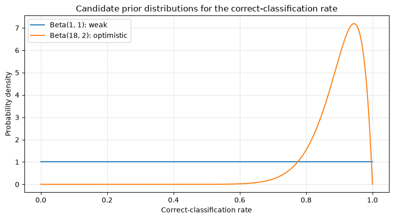

Reading the results

Beta (1,1) treats the entire range equally. Beta (18.2) strongly assumes around 90%. In this example, Beta(1,1) is used to prioritize transparency in comparison, but when using mass production results for preliminary distribution, a design that discounts time and equipment differences is necessary.

No.054: Calculating the posterior distribution of Plan A and Plan B

Meaning in Practice

Once you have the test results, update the ‘plausible range’ for each proposal’s rates. With beta and binary models, calculations can be performed analytically, making explanation, auditing, and recalculation easy.

Approach to Analysis and Modeling

For $x$ successes and $n-x$ failures,

$$p\mid x,n \sim \mathrm{Beta}(\alpha+x,\;\beta+n-x)$$

That’s right. A 95% credit interval can be interpreted as “a 95% probability that the parameter falls within the interval under the posterior distribution.”

Check with Python

prior_a, prior_b = 1, 1
ab["post_a"] = prior_a + ab["correct"]
ab["post_b"] = prior_b + ab["incorrect"]
ab["posterior_mean"] = ab["post_a"] / (ab["post_a"] + ab["post_b"])
ab["ci_low"] = beta.ppf(0.025, ab["post_a"], ab["post_b"])
ab["ci_high"] = beta.ppf(0.975, ab["post_a"], ab["post_b"])
ab[["variant", "inspected", "correct", "posterior_mean", "ci_low", "ci_high"]].style.format(
    {c: "{:.2%}" for c in ["posterior_mean", "ci_low", "ci_high"]}
)

	variant	inspected	correct	posterior_mean	ci_low	ci_high
0	A(Current)	800	750	93.64%	91.85%	95.22%
1	B(New Conditions)	800	763	95.26%	93.69%	96.62%

x = np.linspace(0.88, 0.99, 800)
for label, row in zip(["A: current", "B: new"], ab.itertuples()):
    plt.plot(x, beta.pdf(x, row.post_a, row.post_b), label=label)
plt.title("Posterior distributions of the correct-classification rate")
plt.xlabel("Correct-classification rate")
plt.ylabel("Probability density")
plt.grid(True, alpha=0.3)
plt.legend()
plt.tight_layout()
plt.show()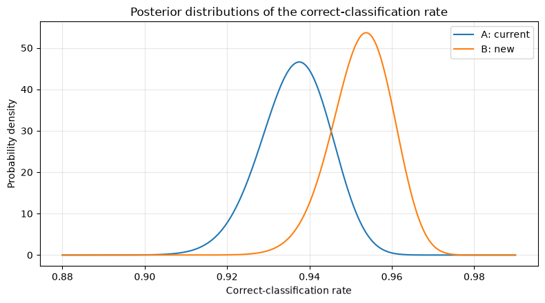

Reading the results

While the post-hoc mean is close to the observation rate, there is a wide range of options for each proposal. Since overlap remains even if the distribution of B leans to the right, we do not treat it definitively based solely on the size of the mean; instead, we check the next superiority probability and the distribution of differences.

No.055: Calculating the Probability That Plan B Is Superior to Plan A

Meaning in Practice

The “probability that B will outperform A” can be intuitively explained in meetings. However, since the probability is that even a small margin is better, the probability of surpassing the difference that is practically meaningful will also be listed.

Approach to Analysis and Modeling

Independently sample $p_A^{(s)},p_B^{(s)}$ from the posterior distribution and find the proportion of $p_B^{(s)}>p_A^{(s)}$. Similarly, the probability that the $p_B-p_A>0.005$ ratio exceeds the minimum practical difference.

Check with Python

draws = 200_000
a_row, b_row = ab.iloc[0], ab.iloc[1]
p_a = rng.beta(a_row.post_a, a_row.post_b, draws)
p_b = rng.beta(b_row.post_a, b_row.post_b, draws)
delta = p_b - p_a

prob_superior = np.mean(delta > 0)
prob_practical = np.mean(delta > 0.005)
pd.DataFrame({
    "indicator": ["P(B > A | data)", "P(B - A > 0.5pt | data)"],
    "value": [prob_superior, prob_practical]
}).style.format({"value": "{:.2%}"})

	indicator	value
0	P(B > A | data)	92.37%
1	P(B - A > 0.5pt | data)	83.90%

Reading the results

Even if the probability of superiority is high, the probability of exceeding the minimum practical difference can be low. The former represents direction, while the latter represents business scale. Whether it is adopted or not, the latter and implementation losses are emphasized.

No.056: Visualizing the Post-Postmortem Distribution of CVR Differences

Meaning in Practice

The distribution of differences simultaneously shows not only improvement but also the potential for deterioration and the extent of improvement. Management, quality assurance, and technical departments can view the same diagram and discuss risk tolerance.

Approach to Analysis and Modeling

$\Delta=p_B-p_A$ samples are histogrammed, showing 0 (equivalent) and 0.5 points (minimum practical difference). We also calculate the 95% credit bracket for the subsolescence.

Check with Python

delta_ci = np.quantile(delta, [0.025, 0.5, 0.975])
plt.hist(delta * 100, bins=70, density=True, alpha=0.75, color="tab:blue")
plt.axvline(0, color="black", linestyle="--", label="No difference")
plt.axvline(0.5, color="tab:red", linestyle=":", label="Practical threshold (0.5 pt)")
plt.title("Posterior distribution of improvement: B - A")
plt.xlabel("Improvement in correct-classification rate (percentage points)")
plt.ylabel("Probability density")
plt.grid(True, alpha=0.3)
plt.legend()
plt.tight_layout()
plt.show()
print(f"Median: {delta_ci[1]*100:.2f} pt")
print(f"95% credible interval: [{delta_ci[0]*100:.2f}, {delta_ci[2]*100:.2f}] pt")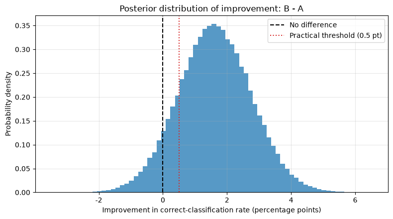

Median: 1.61 pt
95% credible interval: [-0.60, 3.87] pt

Reading the results

The area left of 0 may worsen B, while the area above 0.5 may exceed the practical difference. Even if the section exceeds zero, we do not definitively say it is “ineffective,” but use the probability of upward and downward swings and losses as factors to decide whether to continue or stop.

No.057: Calculating Expected Improvement

Meaning in Practice

By converting the difference in rates into annual quantity and amount, you can link the statistical results to capital investment decisions. On the other hand, calling only the average of $\max(\Delta,0)$ “net benefit” ignores the risk of worsening, so signed expected spread and expected loss are also listed.

Approach to Analysis and Modeling

If the annual number of targets is $N$ and the loss per misplaced item is $c$, the expected gross benefit is $N c E[\Delta]$. Subtract the $C$ implementation cost to calculate the expected net benefit. Here, we assume that other KPIs are equivalent.

Check with Python

annual_units = 1_200_000
loss_per_false_reject = 420
implementation_cost = 5_000_000

annual_avoided = annual_units * delta
gross_benefit = annual_avoided * loss_per_false_reject
net_benefit = gross_benefit - implementation_cost

business_case = pd.DataFrame({
    "indicator": ["Expected improvement", "Annual Misplaced Emissions Reduction", "Looking forward to coarse benefits", "Expected net benefit after deduction of introduction costs", "Probability of positive net benefit"],
    "value": [f"{delta.mean()*100:.2f} pt", f"{annual_avoided.mean():,.0f} units",
          f"{gross_benefit.mean()/1e6:,.2f} million yen", f"{net_benefit.mean()/1e6:,.2f} million yen",
          f"{np.mean(net_benefit > 0):.1%}"]
})
business_case

	indicator	value
0	Expected improvement	1.62 pt
1	Annual Misplaced Emissions Reduction	19,478 units
2	Looking forward to coarse benefits	8.18 million yen
3	Expected net benefit after deduction of introduction costs	3.18 million yen
4	Probability of positive net benefit	71.0%

Reading the results

Even if the improvement rate seems small, the financial impact can be significant if the annual volume is large. Conversely, even if the probability of superiority is high, there are cases where the implementation cost cannot be recovered. In reality, missed losses, downtime, and maintenance costs are also added in the same unit.

No.058: Considering decisions when sample sizes are small

Meaning in Practice

Initial data fluctuates greatly. If winners are determined solely by early observation rates, it becomes easier to adopt a plan that was just a good coincidence. Even Bayesian estimation does not eliminate the lack of data itself.

Approach to Analysis and Modeling

Changing only the sample size from the same true rate compares the superiority probability and the 95% credit interval width of the difference. If you are conducting continuous monitoring, you should set the minimum sample size, maximum sample size, and stop criteria in advance.

Check with Python

sample_sizes = [25, 50, 100, 200, 400, 800, 1600]
records = []
for n in sample_sizes:
    xa = rng.binomial(n, true_rates["A(Current)"])
    xb = rng.binomial(n, true_rates["B(New Conditions)"])
    da = rng.beta(1 + xa, 1 + n - xa, 30_000)
    db = rng.beta(1 + xb, 1 + n - xb, 30_000)
    d = db - da
    lo, hi = np.quantile(d, [0.025, 0.975])
    records.append({"n_per_arm": n, "prob_B_superior": np.mean(d > 0),
                    "interval_width_pt": (hi - lo) * 100})
sequential = pd.DataFrame(records)
sequential.style.format({"prob_B_superior": "{:.1%}", "interval_width_pt": "{:.2f}"})

	n_per_arm	prob_B_superior	interval_width_pt
0	25	50.4%	28.88
1	50	36.6%	23.88
2	100	49.8%	13.94
3	200	97.6%	10.96
4	400	89.3%	7.11
5	800	97.2%	4.85
6	1600	92.1%	3.32

fig, ax1 = plt.subplots()
ax1.plot(sequential["n_per_arm"], sequential["prob_B_superior"], marker="o", color="tab:blue")
ax1.set_xlabel("Sample size per arm")
ax1.set_ylabel("P(B > A | data)", color="tab:blue")
ax1.grid(True, alpha=0.3)
ax2 = ax1.twinx()
ax2.plot(sequential["n_per_arm"], sequential["interval_width_pt"], marker="s", color="tab:orange")
ax2.set_ylabel("95% interval width (percentage points)", color="tab:orange")
plt.title("Uncertainty decreases as sample size grows")
fig.tight_layout()
plt.show()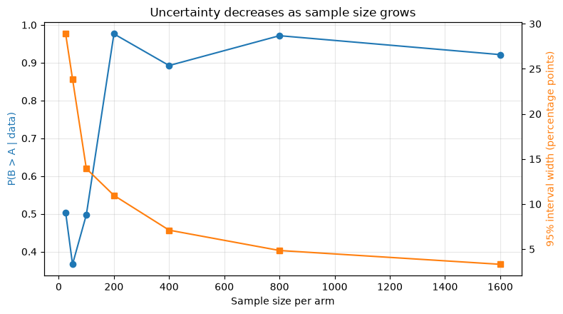

Reading the results

While the odds of superiority move extremely in a small sample, the credit range remains wide. It is also important that a single simulation path does not become monotonous. For example, we set operational rules such as “If there are fewer than 400 proposals, we will not adopt” and “If judgment is impossible, we will continue until the upper limit.”

No.059: Conduct Multiple Patterns of A/B/n Testing

Meaning in Practice

When comparing three or more equipment conditions, you can use the probability that each option is the best. However, the more candidates you add, the fewer tests each option can be conducted, making it easier to include variations in varieties and time slots.

Approach to Analysis and Modeling

Simultaneous sampling is performed from the posterior distribution of each proposal, and the proposal that is the largest in each round is counted. We also check the difference and expected net benefit from current A as well. The “best probability” does not guarantee the size of the difference, so it is not used as a hiring criterion on its own.

Check with Python

variants = pd.DataFrame({
    "variant": ["A Current", "B High sensitivity", "C Balance", "D high-speed"],
    "inspected": [600, 600, 600, 600],
    "correct": [556, 568, 572, 561]
})
variants["incorrect"] = variants["inspected"] - variants["correct"]
post_draws = np.column_stack([
    rng.beta(1 + r.correct, 1 + r.incorrect, 150_000) for r in variants.itertuples()
])
best = np.argmax(post_draws, axis=1)
variants["posterior_mean"] = post_draws.mean(axis=0)
variants["prob_best"] = np.bincount(best, minlength=len(variants)) / len(best)
variants[["variant", "inspected", "correct", "posterior_mean", "prob_best"]].style.format(
    {"posterior_mean": "{:.2%}", "prob_best": "{:.1%}"}
)

	variant	inspected	correct	posterior_mean	prob_best
0	A Current	600	556	92.53%	0.8%
1	B High sensitivity	600	568	94.52%	28.2%
2	C Balance	600	572	95.18%	66.8%
3	D high-speed	600	561	93.36%	4.3%

plot_labels = variants["variant"].str.split().str[0]
plt.bar(plot_labels, variants["prob_best"], color=["gray", "tab:blue", "tab:green", "tab:orange"])
plt.title("Posterior probability that each variant is best")
plt.xlabel("Inspection setting")
plt.ylabel("Probability of being best")
plt.grid(True, axis="y", alpha=0.3)
plt.tight_layout()
plt.show()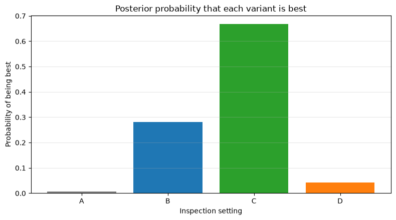

Reading the results

The best probability option is a candidate, but you cannot immediately adopt it by ignoring processing speed, missed rates, and change costs. For multiple comparisons, using the same period and allocation mechanism, and holding a confirmation test after candidate selection can reduce selection bias.

No.060: Designing decision rules for Bayesian A/B tests

Meaning in Practice

To turn analysis into action, you need conditions like “hire,” “continue,” and “post.” Combine not only probability thresholds but also practical differences, expected net benefits, guardrails, and minimum sample size.

Approach to Analysis and Modeling

The rules for this example are as follows.

1. Over 400 cases per case
2. $P(\Delta>0)>95\%$
3. $P(\Delta>0.005)>70\%$
4. $P(\text{pure convenience}>0)>80\%$
5. Meets guardrails for missed rates and processing times

The benchmark is not a universally correct answer; raters set it based on mishiring, loss of abandonment, and the cost of additional testing.

Check with Python

guardrail_pass = True  # Assuming a fitting alternative evaluation
checks = pd.DataFrame({
    "Determination Criteria": ["Each case400more than one", "P(B>A)>95%", "P(B-A>0.5pt)>70%", "P(pure convenience>0)>80%", "Guardrail Compatible"],
    "Achievements": [ab["inspected"].min() >= 400, prob_superior > 0.95, prob_practical > 0.70,
            np.mean(net_benefit > 0) > 0.80, guardrail_pass]
})
decision = "Adoption" if checks["Achievements"].all() else ("Continuing the trial" if ab["inspected"].min() < 1600 else "Seeing off／redesign")
display(checks)
print("This time's judgment:", decision)

	Determination Criteria	Achievements
0	Each case400more than one	True
1	P(B>A)>95%	False
2	P(B-A>0.5pt)>70%	True
3	P(pure convenience>0)>80%	False
4	Guardrail Compatible	True

This time's decision: Trial continues

Reading the results

Recruitment will only be made if all conditions are met. If the requirements are not met, instead of simply saying ‘no significant difference,’ continue or pass by confirming that the value of the additional information exceeds the trial cost. Coded rules prevent arbitrary changes to standards from meeting to meeting.

7. Practical Insights Seen Through Target Exercise

1. Separating probability from value: The probability of B winning, the probability of exceeding the practical difference, and the expected net benefit are different questions.
2. Pricing Uncertainty, Not Erasing: Compare losses in case of deterioration with additional testing costs.
3. Set the rules in advance: Approve KPIs, minimum practical differences, stoppage conditions, and exclusion conditions before the exam.
4. Comparability Ahead of Models: If the validity of random allocation, concurrent comparison, stratification, or measurement systems is compromised, even if calculations are precise, conclusions become weak.
5. localKPIThey just don’t hire them.: Include missed items, takt time, downtime, and training and maintenance costs in guardrails or loss functions.

8. What is necessary for practical implementation

• Appointment of decision-making leaders involved in quality assurance, manufacturing, technology, and accounting
• A study protocol specifying the target population, assigned units, stratification factors, and criteria for missing or exclusion
• Measurement system analysis and logs for time, lot, and equipment ID setup
• Basis for prior distributions and decision thresholds, and sensitivity analysis using separate prior distributions
• Review procedures to simultaneously monitor key KPIs and guardrails
• Post-adoption effectiveness verification, model drift monitoring, rollback conditions

This beta-binomial model assumes independent and homogeneous observations. If rates differ by type, equipment, or shift, extend to stratified models or hierarchical Bayes, or if time dependence is strong, extend to time series models.

9. Summary

No.051–060 covered everything from the definition of A/B test objectives, pre- and posterior distributions, odds of dominance, range of improvement, small samples, A/B/n, and decision-making rules. The strength of Bayes A/B testing is that it can connect results that suggest “B looks good” to How certain is it, how valuable is it, and under what conditions should we act?.

10. Consultations for Corporations

At Suri Kobo, we support everything from manufacturing condition comparison, quality KPI design, sequential testing, Bayesian model construction, decision-making rule design, to on-site training, tailored to the state of the data and operational constraints. We can consult about building a system that goes beyond just PoC, covering approval, operation, and monitoring.

📩 Contact Us: surikobo.co.jp/contact Please feel free to consult us first.