Turning Uncertainty into a “Decision-Making Power”: 10 Key Exercises on Bayesian Decision-Making and Practical Implementation in Manufacturing

This article uses a fictional precision parts factory as a subject to connect the results of Bayesian estimation to Maintenance, inventory, policy selection, explanation, and operational design. The target is No.091 to No.100. Rather than just calculating probabilities, the decision-making process treats everything as a single step: “which actions to choose,” “how much misjudgment costs,” and “whether it can be sustained.”

[!NOTE] This material is a notebook previously used by Surikoubo (or personally by the representative, Kazuyama), and has been reconstructed, edited, and published with the company’s permission.
All data listed is fictional and has no relation whatsoever to real companies, factories, or figures.

Introduction: Practical Challenges in Manufacturing Covered in This Article

Equipment failure rates and demand for replacement parts are observed during short periods and fluctuate depending on season, product type, and operating conditions. Still, the site must decide by deadline whether to implement preventive replacements, how many parts to keep, and which improvements to invest in. Here, using the critical equipment at Factory A as an example, we will Bayes-style updates past data and expert insights, breaking down losses, risks, explanatory materials, and operational requirements. Amounts are in tens of thousands of yen.

Common situations on site

• While fewer failures are desirable, there is also limited data available for training.
• If you place orders based solely on average demand, you tend to focus on either out-of-stock or excess inventory
• Accuracy metrics are reported but are not linked to actual misjudgment costs
• Only analysts understand the model, and responsibilities for updates, approvals, and shutdowns are ambiguous.

Why is this issue so difficult to judge?

If we $p$ unknown failure probabilities, $D$ data, $a$ actions, and $L(a,p)$ losses, Bayesian decision-making

$a^*=\arg\min_a \mathbb{E}_{p\mid D}[L(a,p)]$

Select the option. By using the entire distribution, it is possible to simultaneously handle uncertainties caused by data shortages and asymmetries such as downtime, inventory costs, and missed losses. However, it only works in practice after designing loss monetization, model diagnosis, explanation, and update monitoring.

Overview of Exercise covered this time

No.	Theme	Deciding on site
091	Bayesian Decision-Making	Choosing actions based on post-event distribution and loss
092	expected value	Comparing the average economic efficiency of the policy
093	loss function	Clearly state the weight of out-of-stock and surplus
094	Cost of misjudgment	Set alert thresholds based on operational costs
095	Risk Considerations	Compare not only averages but also downside
096	Forecast Distribution and Inventory	Probabilistic Decision of Ordering Points
097	Model Validity	Checking reproducibility with post-event prediction
098	Explanation for Non-Experts	Translating probabilities into actions, amounts, and deadlines
099	dashboard	Turn decision KPIs into operational screens
100	Project Design	Designing from PoC to Production

Preparing the Python environment

We use NumPy, pandas, SciPy, and matplotlib. Fix the random seed and set the Japanese font, title, axis name, grid, and tight_layout on the graph.

import platform
import numpy as np
import pandas as pd
import scipy
import matplotlib
import matplotlib.pyplot as plt
import japanize_matplotlib
from IPython.display import display

SEED = 20260712
rng = np.random.default_rng(SEED)
pd.set_option("display.float_format", lambda x: f"{x:,.3f}")
print(f"Python: {platform.python_version()}")
print(f"NumPy: {np.__version__}, pandas: {pd.__version__}")
print(f"SciPy: {scipy.__version__}, matplotlib: {matplotlib.__version__}")
print(f"random seed: {SEED}")

Python: 3.11.9
NumPy: 1.26.4, pandas: 2.2.2
SciPy: 1.13.1, matplotlib: 3.9.2
random seed: 20260712

Creation of Fictional Data

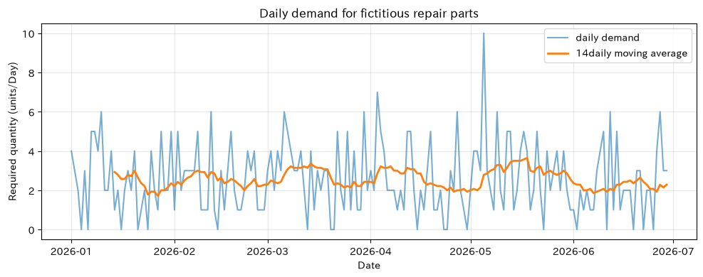
It generates 180 days of spare parts demand and 120 equipment inspections. Including demand fluctuations before and after the weekend planned stoppage, the inspection will be set to ‘Response Needed’ to 1 and ‘Normal’ to 0. In practice, it is assumed to be obtained from ERP, maintenance management, and sensor ledgers, but here it does not rely on external data.

n_days = 180
dates = pd.date_range("2026-01-01", periods=n_days, freq="D")
latent_rate = 2.3 + 0.35 * (dates.dayofweek >= 5) + 0.25 * np.sin(np.arange(n_days)*2*np.pi/30)
demand = rng.poisson(latent_rate)
demand_df = pd.DataFrame({"Date": dates, "demand": demand, "Expected Demand Rate": latent_rate})
n_inspections = 120
issues = rng.binomial(1, 0.105, n_inspections)
inspection_df = pd.DataFrame({"inspectionID": [f"I-{i:03d}" for i in range(1,121)], "Response Required": issues})
display(demand_df.head())
display(pd.DataFrame({"indicator":["Observation Days","Total demand","Average daily demand","Number of inspections","Number of Cases Required"],
                      "value":[n_days,demand.sum(),demand.mean(),n_inspections,issues.sum()]}))
fig, ax = plt.subplots(figsize=(10,4))
ax.plot(dates, demand, alpha=.6, label="daily demand")
ax.plot(dates, pd.Series(demand).rolling(14).mean(), linewidth=2, label="14daily moving average")
ax.set_title("Daily demand for fictitious repair parts"); ax.set_xlabel("Date"); ax.set_ylabel("Required quantity (units/Day)")
ax.grid(True, alpha=.3); ax.legend(); fig.tight_layout(); plt.show()

	Date	demand	Expected Demand Rate
0	2026-01-01	4	2.300
1	2026-01-02	3	2.352
2	2026-01-03	2	2.752
3	2026-01-04	0	2.797
4	2026-01-05	3	2.486

	indicator	value
0	Observation Days	180.000
1	Total demand	465.000
2	Average daily demand	2.583
3	Number of inspections	120.000
4	Number of Cases Required	13.000

No.091: Understanding Bayesian Decision-Making Concepts

Meaning in Practice

A “response rate of about 10%” alone is not enough to decide whether to perform preventive replacements. Compare preventive replacement costs and stoppage losses after the postponement by action and the expected loss over a posterior distribution.

Approach to Analysis and Modeling

$\mathrm{Beta}(2,18)$ the response rate $p$, and assume the Bernoulli distribution based on the inspection results. If the number of cases to be handled is $s$ and the number of normal cases is $f$, then it is $p\mid D\sim\mathrm{Beta}(2+s,18+f)$. For “replacement,” the cost is 400,000 yen; for “postponement,” it is 3.2 million yen for failure.

Check with Python

s, f = int(issues.sum()), int(n_inspections-issues.sum())
p_samples = rng.beta(2+s, 18+f, 100_000)
decision_091 = pd.DataFrame({"action":["preventive replacement","Seeing off"],
 "Expected loss after the fact (ten thousand yen)":[40, (p_samples*320).mean()]})
display(decision_091.sort_values("Expected loss after the fact (ten thousand yen)"))
print(f"Post-Response Average: {p_samples.mean():.1%}")
print(f"95%credit range: {np.quantile(p_samples,.025):.1%}〜{np.quantile(p_samples,.975):.1%}")

	action	Expected loss after the fact (ten thousand yen)
1	Seeing off	34.297
0	preventive replacement	40.000

Post-response average response: 10.7%
95% credit range: 6.2% to 16.3%

Reading the results

Actions with minimal expected loss are recommended for this loss setting. The recommendation depends not only on the model but also on the suspension effect of 3.2 million yen. Record the grounds for the suspension loss and the approver, and recalculate if the assumptions change.

No.092: Making Decisions Based on Expectations

Meaning in Practice

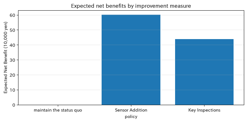
There is uncertainty in the implementation costs and effectiveness of improvement measures. Compare not only the probability of success but also the expected net benefit including success and failure.

Approach to Analysis and Modeling

If the net benefit of the $a$ is $B_a$, you maximize $\mathbb{E}[B_a\mid D]$. However, the expected value is a long-term average and does not guarantee a one-time implementation, so it also indicates the probability of a loss.

Check with Python

n_sim = 80_000
benefits = {"maintain the status quo":np.zeros(n_sim), "Sensor Addition":rng.normal(95,45,n_sim)-35,
            "Key Inspections":rng.normal(62,22,n_sim)-18}
ev_table = pd.DataFrame({"policy":benefits.keys(),
 "Expected Net Benefit (10,000 yen)":[x.mean() for x in benefits.values()],
 "deficit probability":[(x<0).mean() for x in benefits.values()]})
display(ev_table.sort_values("Expected Net Benefit (10,000 yen)", ascending=False))
fig, ax = plt.subplots(figsize=(8,4)); ax.bar(ev_table["policy"], ev_table["Expected Net Benefit (10,000 yen)"])
ax.set_title("Expected net benefits by improvement measure"); ax.set_xlabel("policy"); ax.set_ylabel("Expected Net Benefit (10,000 yen)")
ax.grid(True, axis="y", alpha=.3); fig.tight_layout(); plt.show()

	policy	Expected Net Benefit (10,000 yen)	deficit probability
1	Sensor Addition	60.051	0.091
2	Key Inspections	43.908	0.022
0	maintain the status quo	0.000	0.000

Reading the results

Policies with the highest expected net benefit are generally attractive, but listing the probability of losses together makes it harder to misunderstand uncertainty. If your loss tolerance is low for a one-time investment, you also need the No.095 downside indicator.

No.093: Designing the Loss Function

Meaning in Practice

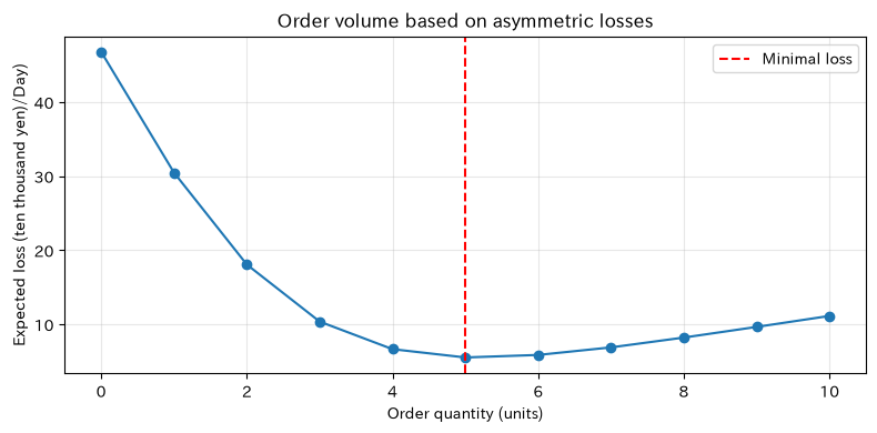
Inventory surpluses and shortages are not symmetrical. If the loss from one unit being missing and the equipment stopping is greater than the cost of one unit left, ordering at average demand is risky.

Approach to Analysis and Modeling

For order $q$, demand $d$, surplus unit price $c_o$, and out-of-stock unit price $c_u$, $L(q,d)=c_o\max(q-d,0)+c_u\max(d-q,0)$ is assumed to be the . Here, $c_o=1.5$ is $c_u=18$ million yen.

Check with Python

future_demand = rng.poisson(rng.gamma(20, demand.mean()/20, 100_000))
orders = np.arange(11); over_cost, under_cost = 1.5, 18.0
expected_loss = [np.mean(over_cost*np.maximum(q-future_demand,0)+under_cost*np.maximum(future_demand-q,0)) for q in orders]
loss_table = pd.DataFrame({"Order Volume":orders,"Expected loss (ten thousand yen)/Day)":expected_loss})
display(loss_table.nsmallest(5,"Expected loss (ten thousand yen)/Day)"))
fig, ax = plt.subplots(figsize=(8,4)); ax.plot(orders, expected_loss, marker="o")
ax.axvline(orders[np.argmin(expected_loss)], color="red", linestyle="--", label="Minimal loss")
ax.set_title("Order volume based on asymmetric losses"); ax.set_xlabel("Order quantity (units)"); ax.set_ylabel("Expected loss (ten thousand yen)/Day)")
ax.grid(True, alpha=.3); ax.legend(); fig.tight_layout(); plt.show()

	Order Volume	Expected loss (ten thousand yen)/Day)
5	5	5.503
6	6	5.844
4	4	6.623
7	7	6.864
8	8	8.191

Reading the results

The minimum point of the loss curve is the recommended order quantity. Because the out-of-stock unit price is high, it tends to lean toward safety over average demand. Unit prices are not set solely by the analysts; manufacturing, maintenance, procurement, and accounting agree on breakdowns of stoppage, emergency transport, and disposal.

No.094: Considering the Cost of Misjudgment

Meaning in Practice

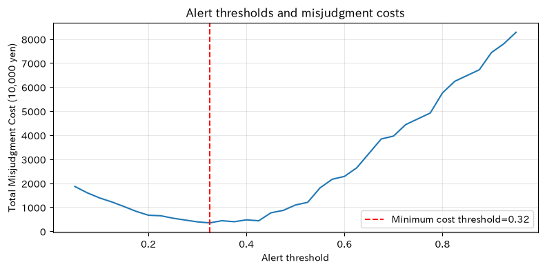
There are two types of abnormal alerts: false positives, which stop when the abnormality is normal, and false negatives, which miss abnormalities. The highest accuracy threshold does not necessarily mean the lowest cost.

Approach to Analysis and Modeling

If the prediction probability is above the threshold $t$, inspect it. Assuming one false positive case equals 30,000 yen and one false negative case equals 1,200,000 yen, the total loss is compared.

Check with Python

n_cases=800; true_issue=rng.binomial(1,.09,n_cases)
score=np.where(true_issue==1,rng.beta(5,2,n_cases),rng.beta(1.5,8,n_cases))
rows=[]
for t in np.linspace(.05,.95,37):
    pred=score>=t; fp=((pred==1)&(true_issue==0)).sum(); fn=((pred==0)&(true_issue==1)).sum()
    rows.append((t,fp,fn,3*fp+120*fn))
threshold_df=pd.DataFrame(rows,columns=["threshold","false positive","false negative","Total Misjudgment Cost (10,000 yen)"])
best_t=threshold_df.loc[threshold_df["Total Misjudgment Cost (10,000 yen)"].idxmin(),"threshold"]
display(threshold_df.nsmallest(5,"Total Misjudgment Cost (10,000 yen)"))
fig,ax=plt.subplots(figsize=(8,4)); ax.plot(threshold_df["threshold"],threshold_df["Total Misjudgment Cost (10,000 yen)"])
ax.axvline(best_t,color="red",linestyle="--",label=f"Minimum cost threshold={best_t:.2f}")
ax.set_title("Alert thresholds and misjudgment costs"); ax.set_xlabel("Alert threshold"); ax.set_ylabel("Total Misjudgment Cost (10,000 yen)")
ax.grid(True,alpha=.3); ax.legend(); fig.tight_layout(); plt.show()

	threshold	false positive	false negative	Total Misjudgment Cost (10,000 yen)
11	0.325	76	1	348
10	0.300	90	1	390
13	0.375	52	2	396
15	0.425	25	3	435
12	0.350	66	2	438

Reading the results

Because the missed value is high, a lower threshold is chosen than when determining based solely on accuracy. In practice, daily alert limits, priority of critical equipment, and approval procedures for threshold changes are also defined.

No.095: Choosing Measures Considering Risks

Meaning in Practice

Even with the same expected profit, it may be rare to adopt measures that cause large losses. We will separate and compare the average and the downside.

Approach to Analysis and Modeling

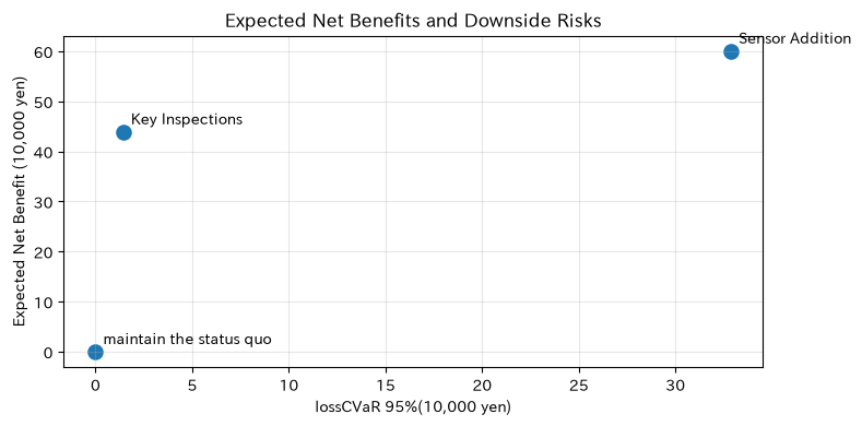
$\mathrm{CVaR}_{0.95}(L)=\mathbb{E}[L\mid L\geq\mathrm{VaR}_{0.95}(L)]$ is the average of the area above 95% VaR of loss $L=-B$.

Check with Python

risk_rows=[]
for name,x in benefits.items():
    loss=-x; var95=np.quantile(loss,.95)
    risk_rows.append((name,x.mean(),np.quantile(x,.05),loss[loss>=var95].mean()))
risk_df=pd.DataFrame(risk_rows,columns=["policy","Expecting pure convenience","pure convenience5%point","lossCVaR95%"])
display(risk_df)
fig,ax=plt.subplots(figsize=(8,4)); ax.scatter(risk_df["lossCVaR95%"],risk_df["Expecting pure convenience"],s=90)
for _,r in risk_df.iterrows(): ax.annotate(r["policy"],(r["lossCVaR95%"],r["Expecting pure convenience"]),xytext=(5,5),textcoords="offset points")
ax.set_title("Expected Net Benefits and Downside Risks"); ax.set_xlabel("lossCVaR 95%(10,000 yen)"); ax.set_ylabel("Expected Net Benefit (10,000 yen)")
ax.grid(True,alpha=.3); fig.tight_layout(); plt.show()

	policy	Expecting pure convenience	pure convenience5%point	lossCVaR95%
0	maintain the status quo	0.000	0.000	0.000
1	Sensor Addition	60.051	-13.884	32.875
2	Key Inspections	43.908	7.603	1.434

Reading the results

The upper right indicates both the average return and the downside of the policy. By clearly stating risk constraints such as “Maximize expected benefits and keep CVaR below the budget limit,” you can reproduce your decision.

No.096: Determining Inventory Levels from Forecast Distribution

Meaning in Practice

Lead time demand is forecasted by distribution and inventory levels matching the ratio of out-of-stock to surplus costs. Service levels can be set based on economic rationality rather than intuition.

Approach to Analysis and Modeling

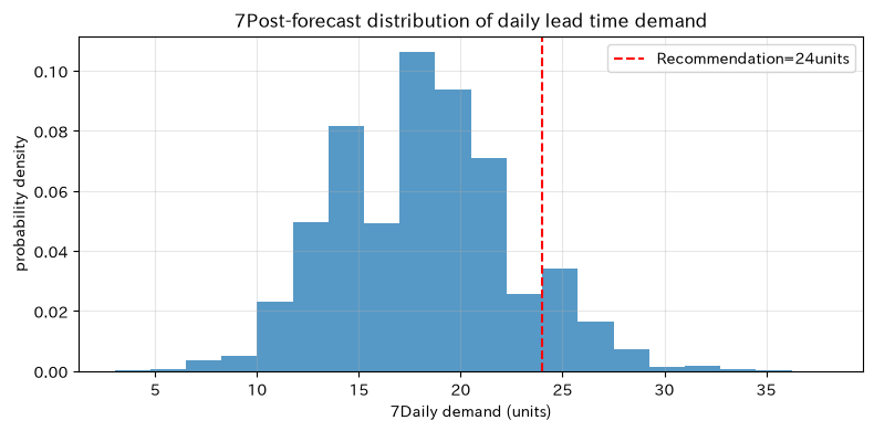
The optimal quantile for the newspaper vendor problem is $q^*=F^{-1}(c_u/(c_u+c_o))$. We forecast demand over 7 days retrospectively and use the same cost as No.093.

Check with Python

rate_samples=rng.gamma(demand.sum()+2,1/(n_days+1),100_000)
lead_time_demand=rng.poisson(7*rate_samples); critical_ratio=under_cost/(under_cost+over_cost)
order_up_to=int(np.quantile(lead_time_demand,critical_ratio,method="higher"))
display(pd.DataFrame({"indicator":["Forecast Average","95%lower limit","95%upper limit","critical ratio","Recommended Inventory Level"],
 "value":[lead_time_demand.mean(),*np.quantile(lead_time_demand,[.025,.975]),critical_ratio,order_up_to]}))
fig,ax=plt.subplots(figsize=(8,4)); ax.hist(lead_time_demand,bins=20,density=True,alpha=.75)
ax.axvline(order_up_to,color="red",linestyle="--",label=f"Recommendation={order_up_to}units")
ax.set_title("7Post-forecast distribution of daily lead time demand"); ax.set_xlabel("7Daily demand (units)"); ax.set_ylabel("probability density")
ax.grid(True,alpha=.3); ax.legend(); fig.tight_layout(); plt.show()

	indicator	value
0	Forecast Average	18.051
1	95%lower limit	10.000
2	95%upper limit	27.000
3	critical ratio	0.923
4	Recommended Inventory Level	24.000

Reading the results

The recommended value is higher than average not because the safety factor was arbitrarily added, but because it reflects that the out-of-stock unit price is greater than the surplus unit price. If the lead time or unit price changes, it will automatically recalculate.

No.097: Validating the Bayesian Model

Meaning in Practice

Even if calculations converge, if the model cannot reproduce the abundance, peak, or variation of zeros, it should not be used for inventory determination.

Approach to Analysis and Modeling

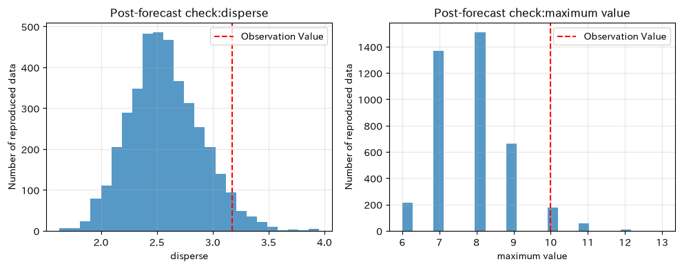
Reproduction data $y^{rep}$ are generated from post-prediction, and the mean, variance, zero ratio, and maximum value are compared with the observed values. The Bayes P value is not a pass/fail test, but a diagnostic value that looks for bias in reproducibility.

Check with Python

n_rep=4000; rep_rates=rng.gamma(demand.sum()+2,1/(n_days+1),n_rep)
y_rep=rng.poisson(rep_rates[:,None],size=(n_rep,n_days))
stats={"average":(demand.mean(),y_rep.mean(1)),"disperse":(demand.var(ddof=1),y_rep.var(1,ddof=1)),
       "zero ratio":((demand==0).mean(),(y_rep==0).mean(1)),"maximum value":(demand.max(),y_rep.max(1))}
ppc_df=pd.DataFrame([(k,o,r.mean(),(r>=o).mean()) for k,(o,r) in stats.items()],
 columns=["statistical quantity","Observation Value","Reproduction value average","Bayespvalue"]); display(ppc_df)
fig,axes=plt.subplots(1,2,figsize=(10,4))
for ax,name in zip(axes,["disperse","maximum value"]):
    o,r=stats[name]; ax.hist(r,bins=25,alpha=.75); ax.axvline(o,color="red",linestyle="--",label="Observation Value")
    ax.set_title(f"Post-forecast check:{name}"); ax.set_xlabel(name); ax.set_ylabel("Number of reproduced data"); ax.grid(True,alpha=.3); ax.legend()
fig.tight_layout(); plt.show()

	statistical quantity	Observation Value	Reproduction value average	Bayespvalue
0	average	2.583	2.579	0.481
1	disperse	3.172	2.574	0.038
2	zero ratio	0.106	0.076	0.117
3	maximum value	10.000	7.859	0.061

Reading the results

Features with Bayesian p-values close to 0 or 1 may be difficult for models to reproduce. If simple poisson does not capture peaks or overdispersions, consider the day-of-the-week effect or negative binomial distribution. Diagnostics continue with each update.

No.098: Explaining Bayesian Analysis Results to Non-Experts

Meaning in Practice

We translate not only “post-posterior distribution” but also recommended behaviors, monetary impact, remaining uncertainty, and review conditions.

Approach to Analysis and Modeling

The explanation will be in the following order: (1) what will be decided, (2) what was learned, (3) recommendations and economic effects, (4) uncertainty, and (5) review conditions. The 95% credit interval is a posterior probability interval that includes unknowns under the conditions of the model and data.

Check with Python

recommended_action=decision_091.loc[decision_091["Expected loss after the fact (ten thousand yen)"].idxmin(),"action"]
avoided_loss=decision_091["Expected loss after the fact (ten thousand yen)"].max()-decision_091["Expected loss after the fact (ten thousand yen)"].min()
decision_card=pd.DataFrame({"item":["Decision-making","Recommendation","Response Rate","uncertainty","Improvement of expected losses","Review Conditions"],
 "Expressions for Management and the Field":["Whether to implement preventive replacement of critical equipment",recommended_action,f"average {p_samples.mean():.1%}",
 f"95%with the probability {np.quantile(p_samples,.025):.1%}〜{np.quantile(p_samples,.975):.1%}",
 f"Alternative Compared to agreement{avoided_loss:.1f}ten_thousand_yen/judgment","inspection30When adding or changing the suspension loss"]})
display(decision_card.style.hide(axis="index"))

item	Expressions for Management and the Field
Decision-making	Whether to implement preventive replacement of critical equipment
Recommendation	Seeing off
Response Rate	average 10.7%
uncertainty	95%with the probability 6.2%〜16.3%
Improvement of expected losses	Alternative Compared to agreement5.7ten_thousand_yen/judgment
Review Conditions	inspection30When adding or changing the suspension loss

Reading the results

Not only recommendations, but also premise and review conditions are placed in the same table. Instead of saying “certain,” we show the current range in intervals, prioritizing the difference and conditions where the judgment reverses compared to the alternative rather than the distribution shape.

No.099: Incorporating Bayesian Analysis into Dashboards

Meaning in Practice

The dashboard is not a collection of graphs, but a screen where the person in charge decides their actions for the day. Displays recommendations, confidence, impact, data freshness, and model health together.

Approach to Analysis and Modeling

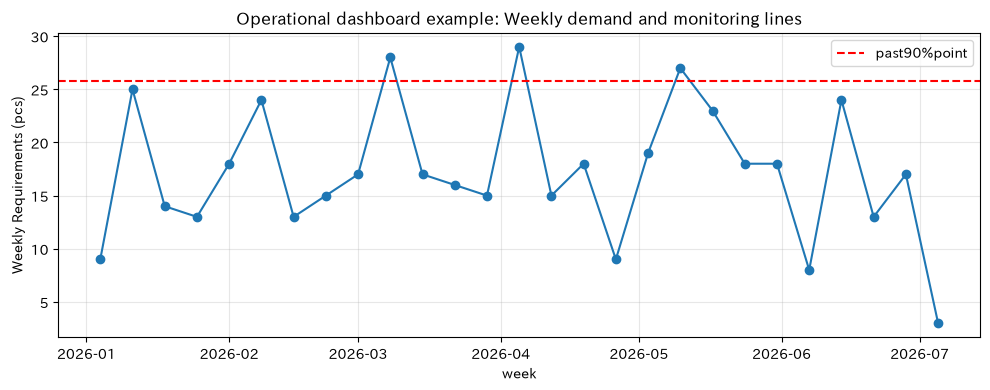
It separates decision-making KPIs, model KPIs, and operational KPIs, managing recommendations and expected losses, predictive diagnostics, and final updates, deficiencies, and human overwrites.

Check with Python

dashboard=pd.DataFrame({"Classification":["Decision-making","Decision-making","Model","Model","Utilization","Utilization"],
 "KPI":["Recommended Actions","Recommended Inventory Level","Response Rate95%upper limit","PPCdispersepvalue","Data Final Day","Loss rate"],
 "present value":[recommended_action,f"{order_up_to}units",f"{np.quantile(p_samples,.975):.1%}",
 f"{ppc_df.loc[ppc_df['statistical quantity']=='disperse','Bayespvalue'].iloc[0]:.2f}",str(dates.max().date()),"0.0%"],
 "Person in charge":["Person responsible for preservation","Procurement Manager","Analysis Specialist","Analysis Specialist","Data controller","Data controller"]}); display(dashboard)
weekly=demand_df.set_index("Date")["demand"].resample("W").sum()
fig,ax=plt.subplots(figsize=(10,4)); ax.plot(weekly.index,weekly.values,marker="o")
ax.axhline(weekly.quantile(.9),color="red",linestyle="--",label="past90%point")
ax.set_title("Operational dashboard example: Weekly demand and monitoring lines"); ax.set_xlabel("week"); ax.set_ylabel("Weekly Requirements (pcs)")
ax.grid(True,alpha=.3); ax.legend(); fig.tight_layout(); plt.show()

	Classification	KPI	present value	Person in charge
0	Decision-making	Recommended Actions	Seeing off	Person responsible for preservation
1	Decision-making	Recommended Inventory Level	24units	Procurement Manager
2	Model	Response Rate95%upper limit	16.3%	Analysis Specialist
3	Model	PPCdispersepvalue	0.04	Analysis Specialist
4	Utilization	Data Final Day	2026-06-29	Data controller
5	Utilization	Loss rate	0.0%	Data controller

Reading the results

Assigning a person in charge for each KPI clarifies how to respond in case of an abnormality. We also record the reasons for overwriting model recommendations. If the update fails or the missing limit is exceeded, the old recommendation will not be displayed silently but will be “Decision Withheld.”

No.100: Designing a Data Analysis Project Using Bayesian Statistics

Meaning in Practice

Even with highly accurate PoCs, production cannot be achieved without decision-making processes, data accountability, monitoring, relearning, and audit trails. First, define “who decides, when, and what.”

Approach to Analysis and Modeling

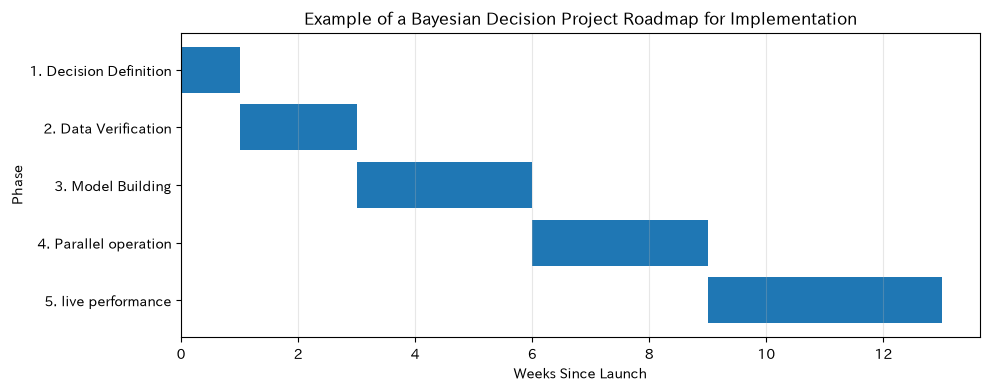
Divided into five stages—decision definition, data validation, model development, parallel operation, and production—each gate is assigned quantitative criteria and approvers. It evaluates not only accuracy but also expected losses, on-site load, critical oversights, and update success rates.

Check with Python

project_plan=pd.DataFrame({"Phase":["1. Decision Definition","2. Data Verification","3. Model Building","4. Parallel operation","5. live performance"],
 "main output":["Loss Table/RACI","Quality Report","Post-event predictionPPC","Decision Logs & Effectiveness Measurement","Monitoring and Suspension Procedures"],
 "Gate Standards (Examples)":["Loss unit price approved by department","Loss rate1%less than","significantPPCNo deviation","expected loss10%The above improvements","Update success rate99%That's all."],
 "approver":["Factory manager","Data Officer","Head of Analysis","Person responsible for preservation","System Officer"]}); display(project_plan.style.hide(axis="index"))
weeks=np.array([1,2,3,3,4]); starts=np.r_[0,np.cumsum(weeks)[:-1]]
fig,ax=plt.subplots(figsize=(10,4)); ax.barh(project_plan["Phase"],weeks,left=starts); ax.invert_yaxis()
ax.set_title("Example of a Bayesian Decision Project Roadmap for Implementation"); ax.set_xlabel("Weeks Since Launch"); ax.set_ylabel("Phase")
ax.grid(True,axis="x",alpha=.3); fig.tight_layout(); plt.show()

Phase	main output	Gate Standards (Examples)	approver
1. Decision Definition	Loss Table/RACI	Loss unit price approved by department	Factory manager
2. Data Verification	Quality Report	Loss rate1%less than	Data Officer
3. Model Building	Post-event predictionPPC	significantPPCNo deviation	Head of Analysis
4. Parallel operation	Decision Logs & Effectiveness Measurement	expected loss10%The above improvements	Person responsible for preservation
5. live performance	Monitoring and Suspension Procedures	Update success rate99%That's all.	System Officer

Reading the results

The actual performance is not completed by the analyst alone. Loss unit prices are approved by the business department, data quality by the data manager, model diagnostics by the analysis manager, and stoppage procedures by the system manager. In parallel operations, we record the difference between recommendations and actual judgments, the reasons behind them, and the results.

Practical Implications Seen Through Target Exercise

1. Separating estimation from decision-making: Even with the same posterior distribution, if losses and constraints change, optimal behavior changes.
2. Don’t decide based solely on averages: Credit range, deficit probability, CVaR, and the bottom of the forecast distribution are listed together.
3. Managing cost assumptions: Leave the basis for stoppage losses or out-of-stock unit prices, the approver, and the revision date.
4. Continuously monitor validity: Use postmortem forecasting, data freshness, defects, and drift as operational KPIs.
5. Translating Explanation into Action: Shows recommendations, differences, deadlines, and review conditions all in one sheet.

What is necessary for practical implementation

• Frequency of decision-making, responsible persons, alternatives, and deadlines for execution
• Breakdown of losses from stoppages, out-of-stock, surpluses, inspections, and misreports and departmental agreements
• Standardization of ID, time, unit, and missing handling among ERP, maintenance, and sensors
• Basis for prior distribution, model versions, inputs, audit trails of judgment results
• Pre-implementation verification through backtesting, post-prediction checks, and parallel operation
• Stop/manual switching procedure in case of update failure, out-of-distribution input, or performance degradation
• Record the authority and reasons for on-site overwriting, with regular effectiveness measurement and re-approval.

Conclusion

The value of Bayesian statistics is not limited to representing unknowns in distribution. By combining loss functions and operational constraints with posterior distribution, you can choose consistent behavior even in uncertain situations. It is important to design a single operational system that includes expected value, downside, inventory quantile, misjudgment cost, model diagnosis, explanation, dashboard, and responsibility allocation.

Consultations for Corporations

At Suri Kobo, we support everything from problem organization to PoC, full-scale operation, and human resource development in demand forecasting, inventory optimization, equipment maintenance, and quality control in manufacturing. You can consult from stages such as “We have predictive models but they are not used for decision-making” or “We are struggling with explanations and approval designs that include uncertainty.”

📩 Contact Us: surikobo.co.jp/contact
Please feel free to consult us first.