Sales and technical support plans that incorporate uncertainty: Reading order amounts, order probabilities, and inquiry numbers through Bayesian regression

Overview

In sales and technical support for manufacturing, it is necessary to estimate “next month’s order amount,” “order probability per project,” and “number of inquiries” based on limited results. In this article, we use a fictional industrial equipment manufacturer as a subject and implement Bayesian linear regression, Bayesian logistic regression, and Bayes-Poisson regression as a single decision-making process. Not only point forecasts but also coefficients and forecast uncertainties are visualized, linking to budget, personnel, and project priorities.

[!NOTE] This material is a notebook previously used by Surikoubo (or personally by the representative, Kazuyama), and has been reconstructed, edited, and published with the company’s permission.
All data listed is fictional and has no relation whatsoever to real companies, factories, or figures.

Introduction: Practical Challenges in Manufacturing Covered in This Article

Industrial equipment has high project prices and long negotiation periods, so plans based on average values have a greater impact if they fail. Here, we forecast order amounts based on monthly sales promotions and activities, determine follow-up rankings based on the probability of receiving estimate projects, and plan technical inquiry staff based on the number of units in operation.

Common situations on site

• There are only a few dozen cases, and the normal regression coefficient fluctuates significantly.
• I want to know the relationship between sales strategies and order amounts, but there is also significant seasonal variation
• We want to properly treat cases as “orders/cancellations” and inquiries as “counts”
• While management meetings require a single number per person, the site needs safety margins

Why is this issue so difficult to judge?

The type of the target variable varies depending on continuous, binary, and counting values, and estimation errors cannot be ignored with small datasets. Bayesian regression combines prior knowledge with observational data, treating unknown parameters as posterior distributions. Therefore, it can be explained using probabilities directly related to decision-making, such as “the probability that the coefficient is positive” or “the probability that the order amount falls below the planned value.”

Overview of Exercise covered this time

No.	Theme	Key Decisions
061–066	Bayesian linear regression	Understanding order value factors, budget planning, and forecasting range
067–068	Bayesian logistic regression	Order Probability and Follow-up Priority for Quotation Projects
069–070	Bayes-Poisson Return	Number of inquiries, number of respondents, and margin for upside

Preparing the Python environment

Fix random number seeds so that the same fictional data can be reproduced in the same environment. Give random_seed to PyMC’s MCMC as well. Graphs are drawn using only matplotlib.

import warnings
warnings.filterwarnings("ignore", category=FutureWarning)

import numpy as np
import pandas as pd
import matplotlib
import matplotlib.pyplot as plt
import pymc as pm
import arviz as az

SEED = 20260712
rng = np.random.default_rng(SEED)
pd.set_option("display.float_format", lambda x: f"{x:,.3f}")

print("numpy      :", np.__version__)
print("pandas     :", pd.__version__)
print("matplotlib :", matplotlib.__version__)
print("PyMC       :", pm.__version__)

numpy      : 2.5.1
pandas     : 3.0.3
matplotlib : 3.11.0
PyMC       : 5.26.1

Creation of Fictional Data

We create three types of business data for the same manufacturer. Linear regression covers monthly order amounts (million yen), logistic regression covers whether quoted projects have been received, and Poisson regression tracks the number of weekly inquiries. This is not based on actual individual company data.

# Monthly Sales Data (36 months)
n_month = 36
sales = pd.DataFrame({
    "month": pd.date_range("2023-01-01", periods=n_month, freq="MS"),
    "promotion_million": rng.uniform(1.5, 7.0, n_month),
    "sales_visits": rng.integers(35, 91, n_month),
})
sales["orders_million"] = (18 + 4.2 * sales["promotion_million"]
                             + 0.32 * sales["sales_visits"]
                             + rng.normal(0, 6.0, n_month))

# Quotation Project Data (160 items)
n_deal = 160
deals = pd.DataFrame({
    "value_million": rng.lognormal(np.log(8), 0.55, n_deal),
    "demo_done": rng.binomial(1, 0.58, n_deal),
    "lead_days": rng.integers(5, 61, n_deal),
})
z = -0.7 - 0.055 * (deals["value_million"] - 8) + 1.25 * deals["demo_done"] - 0.025 * (deals["lead_days"] - 25)
deals["won"] = rng.binomial(1, 1 / (1 + np.exp(-z)))

# Weekly Inquiry Data (80 weeks)
n_week = 80
support = pd.DataFrame({
    "week": np.arange(1, n_week + 1),
    "installed_100": rng.uniform(5, 22, n_week),
    "release_week": rng.binomial(1, 0.18, n_week),
})
lam = np.exp(0.35 + 0.075 * support["installed_100"] + 0.48 * support["release_week"])
support["inquiries"] = rng.poisson(lam)

display(sales.head(3))
display(deals.head(3))
display(support.head(3))

	month	promotion_million	sales_visits	orders_million
0	2023-01-01	5.309	83	64.583
1	2023-02-01	4.153	85	62.291
2	2023-03-01	6.281	62	58.671

	value_million	demo_done	lead_days	won
0	15.960	1	34	1
1	14.069	1	52	0
2	7.036	1	16	1

	week	installed_100	release_week	inquiries
0	1	16.799	0	9
1	2	12.655	0	4
2	3	6.783	1	9

No.061: Understanding the Bayesian Linear Regression Concept

Meaning in Practice

If you can explain the order amount as promotional expenses and number of visits, you can convert next month’s initiative proposals into sales plans. However, it is important not to treat estimates as definite values, and to leave uncertainty based on the amount of data used.

Approach to Analysis and Modeling

$y_i$ the order amount per month $i$, and using standardized promotional expenses and the number of visits as $x_{i1},x_{i2}$,

\mu_i=\alpha+\beta_1x_{i1}+\beta_2x_{i2}$$ That's how it is placed. While frequentist regression focuses on point estimation of coefficients, Bayesian regression seeks $p(\alpha,\boldsymbol{\beta},\sigma\mid y,X)$. ### Check with Python ```python fig, ax = plt.subplots(figsize=(7, 4)) sc = ax.scatter(sales["promotion_million"], sales["orders_million"], c=sales["sales_visits"], cmap="viridis", s=55) fig.colorbar(sc, ax=ax, label="Sales visits") ax.set_title("Monthly orders and promotion spending") ax.set_xlabel("Promotion spending (million JPY)") ax.set_ylabel("Orders (million JPY)") ax.grid(True, alpha=0.3) plt.tight_layout() plt.show() ``` 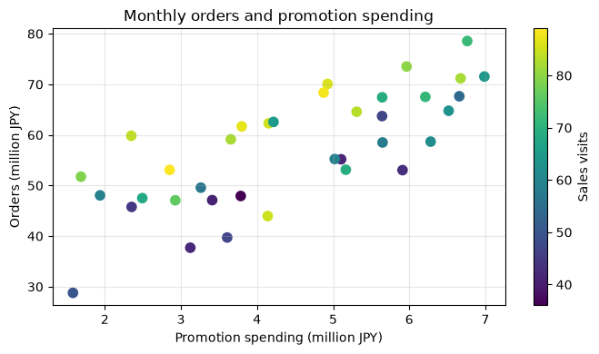 ### Reading the results Months with higher promotional expenses tend to have higher order amounts, but even within the same promotional budget, the number of visits and unexpected fluctuations can vary. This range is carried over into coefficient estimation and future projection called Bayesian regression. It is also important to note that correlation alone cannot be definitively identified as causal effect. ## No.062: Setting a Preliminary Distribution for Regression Coefficients ### Meaning in Practice We suppress unrealistic coefficients such as "orders increase by hundreds of millions yen per 1 million yen of promotional expenses" based on small datasets, and clearly indicate past experiences and operational limits in the model. ### Approach to Analysis and Modeling After standardizing the explanatory variables, set $\alpha\sim\mathcal{N}(50,30)$ for intercepts, $\beta_j\sim\mathcal{N}(0,15)$ for coefficients, and $\sigma\sim\mathrm{HalfNormal}(15)$ for errors. This is a weak information pre-distribution that does not determine the positive or negative coefficients. Through pre-forecast checks, we check whether we generate a large amount of unnatural order amounts. ### Check with Python ```python features = ["promotion_million", "sales_visits"] X_mean, X_sd = sales[features].mean(), sales[features].std() X = ((sales[features] - X_mean) / X_sd).to_numpy() y = sales["orders_million"].to_numpy() prior_rng = np.random.default_rng(SEED + 1) alpha_prior = prior_rng.normal(50, 30, 4000) beta_prior = prior_rng.normal(0, 15, (4000, 2)) sigma_prior = np.abs(prior_rng.normal(0, 15, 4000)) mu_typical = alpha_prior # Standardized explanatory variable 0 (average month) y_prior = prior_rng.normal(mu_typical, sigma_prior) print(pd.Series(y_prior).quantile([0.025, 0.5, 0.975]).rename("prior orders")) ``` 0.025 -15.451 0.500 50.607 0.975 113.715 Name: prior orders, dtype: float64 ### Reading the results Advance forecasts for the average month of activity have a wide range. This means "there is significant uncertainty before looking at the data, but the distinct values are not placed at the center." In practice, we review the distribution in advance with stakeholders based on the range and equipment capacity from the past three years. ## No.063: Implementing Bayesian Linear Regression in PyMC ### Meaning in Practice Turn assumptions into reproducible code and transform model updates from dependent spreadsheets into periodically executable analytical processes. ### Approach to Analysis and Modeling Probability and prior distribution are declared in PyMC, and NUTS samples from posterior distributions. `r_hat` indicates the convergence of multiple chains, and `ess_bulk` indicates the effective sample size. ### Check with Python ```python with pm.Model() as linear_model: alpha = pm.Normal("alpha", mu=50, sigma=30) beta = pm.Normal("beta", mu=0, sigma=15, shape=2) sigma = pm.HalfNormal("sigma", sigma=15) mu = alpha + pm.math.dot(X, beta) pm.Normal("orders", mu=mu, sigma=sigma, observed=y) linear_idata = pm.sample(700, tune=700, chains=2, cores=1, random_seed=SEED, target_accept=0.9, progressbar=False) linear_summary = az.summary(linear_idata, var_names=["alpha", "beta", "sigma"], hdi_prob=0.95, round_to=3) display(linear_summary) ``` Initializing NUTS using jitter+adapt_diag... Sequential sampling (2 chains in 1 job) NUTS: [alpha, beta, sigma] Sampling 2 chains for 700 tune and 700 draw iterations (1_400 + 1_400 draws total) took 16 seconds. We recommend running at least 4 chains for robust computation of convergence diagnostics <style scoped> .dataframe tbody tr th:only-of-type { vertical-align: middle; } .dataframe tbody tr th { vertical-align: top; } .dataframe thead th { text-align: right; } </style> <table border="1" class="dataframe"> <thead> <tr style="text-align: right;"> <th></th> <th>mean</th> <th>sd</th> <th>hdi_2.5%</th> <th>hdi_97.5%</th> <th>mcse_mean</th> <th>mcse_sd</th> <th>ess_bulk</th> <th>ess_tail</th> <th>r_hat</th> </tr> </thead> <tbody> <tr> <th>alpha</th> <td>57.116</td> <td>1.005</td> <td>54.979</td> <td>58.955</td> <td>0.029</td> <td>0.027</td> <td>1,248.667</td> <td>1,024.931</td> <td>1.000</td> </tr> <tr> <th>beta[0]</th> <td>8.216</td> <td>0.980</td> <td>6.286</td> <td>10.115</td> <td>0.028</td> <td>0.029</td> <td>1,268.098</td> <td>816.110</td> <td>1.001</td> </tr> <tr> <th>beta[1]</th> <td>4.974</td> <td>1.018</td> <td>3.251</td> <td>7.253</td> <td>0.028</td> <td>0.029</td> <td>1,313.071</td> <td>815.351</td> <td>1.000</td> </tr> <tr> <th>sigma</th> <td>5.904</td> <td>0.765</td> <td>4.544</td> <td>7.504</td> <td>0.026</td> <td>0.023</td> <td>917.377</td> <td>778.611</td> <td>1.002</td> </tr> </tbody> </table> ### Reading the results If the `r_hat` is generally 1.01 or below and the effective sample size is not extremely small, you can first confirm the numerical convergence. However, convergence does not prove model validity. Residuals, outliers, time dependence, and the data generation process are checked separately. ## No.064: Checking the posterior distribution of the regression coefficient ### Meaning in Practice Instead of choosing between 'effective' or 'not effective,' you can share how confident you are about the magnitude and direction of the effect. ### Approach to Analysis and Modeling For the posterior distribution of the normalization coefficient, check the probability that the 95% HDI (highest post-posterior density interval) is positive. Coefficients are conditional relationships that keep other explanatory variables constant. ### Check with Python ```python beta_draws = linear_idata.posterior["beta"].stack(sample=("chain", "draw")).values coef_result = pd.DataFrame({ "feature": features, "posterior_mean": beta_draws.mean(axis=1), "hdi_2.5%": np.quantile(beta_draws, 0.025, axis=1), "hdi_97.5%": np.quantile(beta_draws, 0.975, axis=1), "P(beta>0)": (beta_draws > 0).mean(axis=1), }) display(coef_result) ``` <style scoped> .dataframe tbody tr th:only-of-type { vertical-align: middle; } .dataframe tbody tr th { vertical-align: top; } .dataframe thead th { text-align: right; } </style> <table border="1" class="dataframe"> <thead> <tr style="text-align: right;"> <th></th> <th>feature</th> <th>posterior_mean</th> <th>hdi_2.5%</th> <th>hdi_97.5%</th> <th>P(beta&gt;0)</th> </tr> </thead> <tbody> <tr> <th>0</th> <td>promotion_million</td> <td>8.216</td> <td>6.188</td> <td>10.107</td> <td>1.000</td> </tr> <tr> <th>1</th> <td>sales_visits</td> <td>4.974</td> <td>2.954</td> <td>7.050</td> <td>1.000</td> </tr> </tbody> </table> ### Reading the results Variables with a higher probability of being positive and whose intervals are far from zero can be observed more stably positive correlations. Since it's a normalization coefficient, you can compare activity by one standard deviation. On the other hand, when promotional expenses and the number of visits are decided simultaneously, experimentation and coordination are necessary to achieve causal effects on the initiative. ## No.065: Visualizing the Bayesian Regression Credit Zone ### Meaning in Practice By showing not only core forecasts for each budget proposal but also the average response credit range, management and the field can share risk levels. ### Approach to Analysis and Modeling Fix the average number of visits and adjust the promotional budget. For each post-coefficient sample, calculate the expected order amount and plot the 2.5, 50, and 97.5 percentiles. This is the uncertainty of the average response and does not include random errors in individual months. ### Check with Python ```python promo_grid = np.linspace(1.5, 7.0, 80) X_grid = np.column_stack([ (promo_grid - X_mean["promotion_million"]) / X_sd["promotion_million"], np.zeros_like(promo_grid), ]) alpha_draws = linear_idata.posterior["alpha"].stack(sample=("chain", "draw")).values mu_grid = alpha_draws[:, None] + beta_draws.T @ X_grid.T lo, med, hi = np.quantile(mu_grid, [0.025, 0.5, 0.975], axis=0) fig, ax = plt.subplots(figsize=(7, 4)) ax.scatter(sales["promotion_million"], y, alpha=0.55, label="Observed") ax.plot(promo_grid, med, color="C1", label="Posterior median") ax.fill_between(promo_grid, lo, hi, color="C1", alpha=0.25, label="95% credible interval") ax.set_title("Expected monthly orders at average sales visits") ax.set_xlabel("Promotion spending (million JPY)") ax.set_ylabel("Expected orders (million JPY)") ax.grid(True, alpha=0.3); ax.legend() plt.tight_layout(); plt.show() ``` 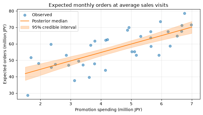 ### Reading the results The band represents the uncertainty of coefficient estimation. The more extrapolate the area with fewer observations, the wider the section generally becomes. A credit interval is a 'post-hoc probability interval where the expected value is included under this model and data,' and it is interpreted differently from the confidence interval in frequentism. ## No.066: Predicting Order Value Using Bayesian Regression ### Meaning in Practice The next month's plan is not set as a single value; instead, it shows downward, median, and upward trends, creating scenarios for cash flow and production capacity. ### Approach to Analysis and Modeling Next month, we will spend 5 million yen on sales promotion and have 70 visits. A post-hoc distribution is created by adding the uncertainty of expected values to the observational error of $\sigma$. The forecast range is broader than the credit range and includes variation in individual months. ### Check with Python ```python next_x = np.array([(5.0 - X_mean["promotion_million"]) / X_sd["promotion_million"], (70 - X_mean["sales_visits"]) / X_sd["sales_visits"]]) sigma_draws = linear_idata.posterior["sigma"].stack(sample=("chain", "draw")).values next_mu = alpha_draws + beta_draws.T @ next_x pred_rng = np.random.default_rng(SEED + 2) next_orders = pred_rng.normal(next_mu, sigma_draws) q = np.quantile(next_orders, [0.025, 0.5, 0.975]) decision = pd.Series({"2.5%": q[0], "median": q[1], "97.5%": q[2], "P(orders < 50)": (next_orders < 50).mean()}) display(decision.to_frame("next-month prediction")) ``` <style scoped> .dataframe tbody tr th:only-of-type { vertical-align: middle; } .dataframe tbody tr th { vertical-align: top; } .dataframe thead th { text-align: right; } </style> <table border="1" class="dataframe"> <thead> <tr style="text-align: right;"> <th></th> <th>next-month prediction</th> </tr> </thead> <tbody> <tr> <th>2.5%</th> <td>49.198</td> </tr> <tr> <th>median</th> <td>61.317</td> </tr> <tr> <th>97.5%</th> <td>72.412</td> </tr> <tr> <th>P(orders &lt; 50)</th> <td>0.034</td> </tr> </tbody> </table> ### Reading the results The median can be used as the baseline plan, and the 2.5% point as a severe downward case. Also, the "probability of falling under 50 million yen" is directly linked to the activation conditions of inventory and financial plans. In decision-making, not only forecast accuracy but also the difference between excess inventory and out-of-stock losses is clearly stated. ## No.067: Understanding Bayesian Logistic Regression ### Meaning in Practice If you use binary results like orders and lost orders as they are in linear regression, the prediction can be less than 0 or even over 1. With logistic regression, you can evaluate the deal as a probability. ### Approach to Analysis and Modeling Taking the $y_i\in\{0,1\}$ of project $i$ as the , $$y_i\sim\mathrm{Bernoulli}(p_i),\qquad \mathrm{logit}(p_i)=\alpha+\boldsymbol{x}_i^\top\boldsymbol{\beta}$$ Let's say so. The $\exp(\beta)$ of the coefficient exponentially is the odds ratio when the explanatory variable increases by one unit under other constant conditions. ### Check with Python ```python win_by_demo = deals.groupby("demo_done")["won"].agg(["count", "mean"]) win_by_demo.index = ["No demo", "Demo completed"] display(win_by_demo.rename(columns={"mean": "observed_win_rate"})) ``` <style scoped> .dataframe tbody tr th:only-of-type { vertical-align: middle; } .dataframe tbody tr th { vertical-align: top; } .dataframe thead th { text-align: right; } </style> <table border="1" class="dataframe"> <thead> <tr style="text-align: right;"> <th></th> <th>count</th> <th>observed_win_rate</th> </tr> </thead> <tbody> <tr> <th>No demo</th> <td>66</td> <td>0.318</td> </tr> <tr> <th>Demo completed</th> <td>94</td> <td>0.479</td> </tr> </tbody> </table> ### Reading the results The observed order rate for demo projects serves as a comparative point, but it does not adjust for differences in project amounts or lead days composition. Regression models handle multiple conditions simultaneously to obtain the order probability distribution for each project. It should be noted that it is not possible to definitively determine the causal effect of the demo from observational data. ## No.068: Estimating Purchase Probability Using Bayesian Logistic Regression ### Meaning in Practice Here, we interpret B2B "purchase" as receiving quotation projects. Not only do we arrange projects in order of probability, but we also calculate the expected order amount by multiplying the project amounts and allocating limited sales work. ### Approach to Analysis and Modeling Standardize deal amounts and lead days, and invest in demo implementation at 0/1. Using the Weak Information Pre-Distribution $\mathcal{N}(0,1.5)$, the probability of winning a deal is calculated for each post-event sample. ### Check with Python ```python logit_cols = ["value_million", "demo_done", "lead_days"] logit_mean = deals[["value_million", "lead_days"]].mean() logit_sd = deals[["value_million", "lead_days"]].std() X_logit = np.column_stack([ (deals["value_million"] - logit_mean["value_million"]) / logit_sd["value_million"], deals["demo_done"], (deals["lead_days"] - logit_mean["lead_days"]) / logit_sd["lead_days"], ]) with pm.Model() as logit_model: a = pm.Normal("a", 0, 1.5) b = pm.Normal("b", 0, 1.5, shape=3) p = pm.Deterministic("p", pm.math.sigmoid(a + pm.math.dot(X_logit, b))) pm.Bernoulli("won", p=p, observed=deals["won"].to_numpy()) logit_idata = pm.sample(700, tune=700, chains=2, cores=1, random_seed=SEED + 3, target_accept=0.9, progressbar=False) p_draws = logit_idata.posterior["p"].stack(sample=("chain", "draw")).values deals_result = deals.copy() deals_result["win_prob"] = p_draws.mean(axis=1) deals_result["expected_orders_million"] = deals_result["value_million"] * deals_result["win_prob"] display(deals_result.nlargest(8, "expected_orders_million") [["value_million", "demo_done", "lead_days", "win_prob", "expected_orders_million"]]) ``` Initializing NUTS using jitter+adapt_diag... Sequential sampling (2 chains in 1 job) NUTS: [a, b] Sampling 2 chains for 700 tune and 700 draw iterations (1_400 + 1_400 draws total) took 89 seconds. We recommend running at least 4 chains for robust computation of convergence diagnostics <style scoped> .dataframe tbody tr th:only-of-type { vertical-align: middle; } .dataframe tbody tr th { vertical-align: top; } .dataframe thead th { text-align: right; } </style> <table border="1" class="dataframe"> <thead> <tr style="text-align: right;"> <th></th> <th>value_million</th> <th>demo_done</th> <th>lead_days</th> <th>win_prob</th> <th>expected_orders_million</th> </tr> </thead> <tbody> <tr> <th>143</th> <td>42.899</td> <td>1</td> <td>5</td> <td>0.554</td> <td>23.760</td> </tr> <tr> <th>156</th> <td>49.475</td> <td>1</td> <td>35</td> <td>0.394</td> <td>19.492</td> </tr> <tr> <th>93</th> <td>21.275</td> <td>1</td> <td>18</td> <td>0.538</td> <td>11.448</td> </tr> <tr> <th>144</th> <td>18.953</td> <td>1</td> <td>25</td> <td>0.503</td> <td>9.537</td> </tr> <tr> <th>149</th> <td>17.189</td> <td>1</td> <td>22</td> <td>0.525</td> <td>9.029</td> </tr> <tr> <th>11</th> <td>16.943</td> <td>1</td> <td>27</td> <td>0.496</td> <td>8.410</td> </tr> <tr> <th>41</th> <td>16.084</td> <td>1</td> <td>25</td> <td>0.510</td> <td>8.208</td> </tr> <tr> <th>76</th> <td>15.074</td> <td>1</td> <td>22</td> <td>0.531</td> <td>7.999</td> </tr> </tbody> </table> ### Reading the results Priority shifts between small projects with high probabilities and large projects with medium probabilities. Expected order value is a useful primary indicator, but strategic customers, gross margin, follow-up time, and delivery constraints are also included in the management. It is important to verify probability calibration over time and not use it hastily for personnel evaluations. ## No.069: Understanding Bayes-Poisson Regression ### Meaning in Practice It handles non-negative integers such as inquiries, failures, and defects. As the number of operating units increases, the number of projects also rises, so simple averages alone can lead to errors in staffing planning. ### Approach to Analysis and Modeling Using the number of $i$ cases per week as $y_i$, $$y_i\sim\mathrm{Poisson}(\lambda_i),\qquad \log\lambda_i=\alpha+\boldsymbol{x}_i^\top\boldsymbol{\beta}$$ Let's say so. $\exp(\beta)$ is the expected multiplier for an increase of one unit in the explanatory variable. Since the Poisson distribution has equal variance to the mean, if overdispersion is strong, negative binomial regression is considered. ### Check with Python ```python count_check = support["inquiries"].agg(["mean", "var", "min", "max"]) display(count_check.to_frame("inquiries")) fig, ax = plt.subplots(figsize=(7, 3.8)) ax.scatter(support["installed_100"], support["inquiries"], c=support["release_week"], cmap="coolwarm", alpha=0.75) ax.set_title("Weekly inquiries and installed base") ax.set_xlabel("Installed units (hundreds)") ax.set_ylabel("Inquiries per week") ax.grid(True, alpha=0.3) plt.tight_layout(); plt.show() ``` <style scoped> .dataframe tbody tr th:only-of-type { vertical-align: middle; } .dataframe tbody tr th { vertical-align: top; } .dataframe thead th { text-align: right; } </style> <table border="1" class="dataframe"> <thead> <tr style="text-align: right;"> <th></th> <th>inquiries</th> </tr> </thead> <tbody> <tr> <th>mean</th> <td>4.050</td> </tr> <tr> <th>var</th> <td>7.263</td> </tr> <tr> <th>min</th> <td>0.000</td> </tr> <tr> <th>max</th> <td>15.000</td> </tr> </tbody> </table> 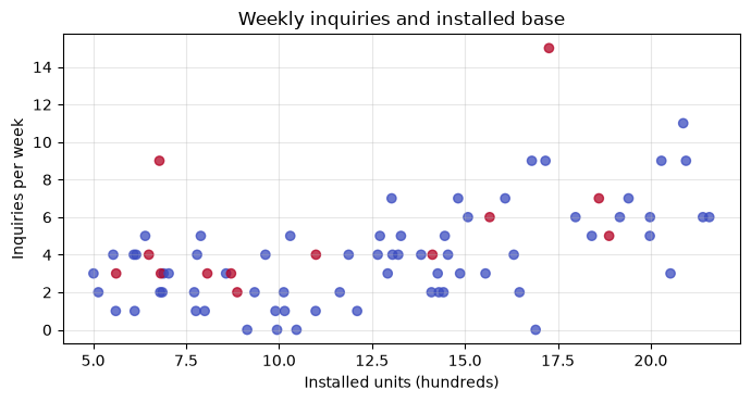 ### Reading the results The week with more active units tends to see an increase in transaction counts, and an upside is visible in release weeks. If the sample variance far exceeds the mean, we suspect insufficient explanatory variables, excess zeros, and weekly heterogeneity. Distribution selection is made based on understanding business processes and post-prediction checks. ## No.070: Estimating the Number of Inquiries Using Bayes-Poisson Regression ### Meaning in Practice Predict the upward swing in inquiries during the new release week using probability distributions, and plan first responders, escalation slots, and outsourcing slots. ### Approach to Analysis and Modeling Standardize the number of units operating and include the logarithmic link along with the release week flag. Not only the expected number of cases for the next week, but also a post-event distribution including Poisson accidental fluctuations is created, and the probability of processing capacity exceedance is calculated. ### Check with Python ```python inst_mean, inst_sd = support["installed_100"].mean(), support["installed_100"].std() X_count = np.column_stack([(support["installed_100"] - inst_mean) / inst_sd, support["release_week"]]) with pm.Model() as count_model: ca = pm.Normal("ca", 0, 1.5) cb = pm.Normal("cb", 0, 1.0, shape=2) rate = pm.Deterministic("rate", pm.math.exp(ca + pm.math.dot(X_count, cb))) pm.Poisson("inquiries", mu=rate, observed=support["inquiries"].to_numpy()) count_idata = pm.sample(700, tune=700, chains=2, cores=1, random_seed=SEED + 4, target_accept=0.9, progressbar=False) ca_d = count_idata.posterior["ca"].stack(sample=("chain", "draw")).values cb_d = count_idata.posterior["cb"].stack(sample=("chain", "draw")).values next_count_x = np.array([(20 - inst_mean) / inst_sd, 1]) next_rate = np.exp(ca_d + cb_d.T @ next_count_x) count_rng = np.random.default_rng(SEED + 5) next_count = count_rng.poisson(next_rate) capacity = 8 count_plan = pd.Series({ "expected inquiries": next_count.mean(), "median": np.median(next_count), "95% prediction lower": np.quantile(next_count, 0.025), "95% prediction upper": np.quantile(next_count, 0.975), f"P(inquiries > {capacity})": (next_count > capacity).mean(), }) display(count_plan.to_frame("release-week plan")) fig, ax = plt.subplots(figsize=(7, 3.8)) bins = np.arange(next_count.min(), next_count.max() + 2) - 0.5 ax.hist(next_count, bins=bins, density=True, alpha=0.75, color="C2") ax.axvline(capacity, color="C3", linestyle="--", label=f"Capacity = {capacity}") ax.set_title("Posterior predictive inquiries: next release week") ax.set_xlabel("Inquiries per week") ax.set_ylabel("Probability") ax.grid(True, alpha=0.3); ax.legend() plt.tight_layout(); plt.show() ``` Initializing NUTS using jitter+adapt_diag... Sequential sampling (2 chains in 1 job) NUTS: [ca, cb] Sampling 2 chains for 700 tune and 700 draw iterations (1_400 + 1_400 draws total) took 33 seconds. We recommend running at least 4 chains for robust computation of convergence diagnostics <style scoped> .dataframe tbody tr th:only-of-type { vertical-align: middle; } .dataframe tbody tr th { vertical-align: top; } .dataframe thead th { text-align: right; } </style> <table border="1" class="dataframe"> <thead> <tr style="text-align: right;"> <th></th> <th>release-week plan</th> </tr> </thead> <tbody> <tr> <th>expected inquiries</th> <td>9.399</td> </tr> <tr> <th>median</th> <td>9.000</td> </tr> <tr> <th>95% prediction lower</th> <td>4.000</td> </tr> <tr> <th>95% prediction upper</th> <td>16.000</td> </tr> <tr> <th>P(inquiries &gt; 8)</th> <td>0.586</td> </tr> </tbody> </table> 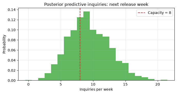 ### Reading the results The 95% prediction range is a realistic range of respondents, and the probability of exceeding eight cases is a key factor in securing support personnel. The threshold is set based on "one loss exceeding the limit" and "the cost of one surplus personnel." Not only the number of transactions, but also processing times by difficulty will be modeled in the next stage. ## Practical Implications Seen Through Target Exercise 1. Depending on the type of the objective variable, you need to select normal for continuous values, Bernoulli for binary values, and Poisson likelihood for number of cases. 2. Rather than point prediction, the probability of downside, the probability of overcapability, and the coefficient coefficient are more helpful for decision-making. 3. Prior distribution does not hide arbitrariness; it visualizes assumptions before viewing the data and serves as a subject for stakeholders to review. 4. Predictive correlation and causal effect are separate. To understand the effectiveness of a policy, experimental design and cross-contamination coordination are necessary. ## What is necessary for practical implementation - **unified definition**: Fix KPI definitions such as order dates, lost orders, and inquiry entries - **point integration**: Use only explanatory variables that were available at the time of prediction to prevent information leaks. - **verification**: Check errors, interval coverage, and probability corrections with time series holdouts - **Diagnosis**: Examines MCMC convergence, post hoc predictions, outliers, overdispersions, and correlations among explanatory variables. - **Utilization**: Break down thresholds, retraining frequency, approvers, and model stop conditions into business procedures - **Governance**: The model assists the person in charge and does not automatically determine ratings or credit approvals. ## Conclusion No.061–070 connect Bayesian regression from a "technique for estimating coefficients" to a "mechanism for allocating business resources including uncertainty." Although order amount, order probability, and number of inquiries differ in data type, they can be organized under a common framework of prior distribution, likelihood, post-post distribution, and post-event forecasting. In practice, the key to success is not only model accuracy but also designing who changes what in response to predictions. ## Consultations for Corporations At Suri Kobo, we support data analysis training for manufacturing companies, Bayesian modeling, demand and order forecasting, decision rule design, and everything from PoC to operational implementation. We also offer consultations on designing objective variables, likelihoods, and preliminary distributions suitable for your company's data, as well as mapping them into dashboards that can be explained by the field. > 📩 **Contact Us**: [surikobo.co.jp/contact](https://surikobo.co.jp/contact) > Please feel free to consult us first.