100 Exercises / SQL / 100 Exercise-Ups to SQL for Data Analysis

Extracting and analyzing defective data from the inspection record database using SQL

2020-01-06

Extracting and analyzing defective data from the inspection record database using SQL

SQL 100 Exercises Chapter 1 (No.001–No.010): SQL Basics

This article is No.1chapter in the “100 Exercises for SQL Basics for Data Analysis” series.
Starting with the SELECT statement, which is the most basic SQL instruction,
FROM, LIMIT, ORDER BY, DISTINCT, and more,
Systematically learn the basics of data acquisition through manufacturing quality control data.

[!NOTE] This material is based on a notebook previously used by Surikoubo (or personally by the representative, Kazuyama), during corporate training.
With the permission of the company, we have restructured and edited the content before publishing.
All data listed is fictional and has no relation whatsoever to real companies, factories, or figures.

Introduction: Practical Challenges in Manufacturing Covered in This Article

This is the case of Mr. Tanaka from the Quality Control Department at an automotive parts manufacturer.

Preparation of monthly quality reports (regular task at the beginning of each month)
  1. Obtain one month's worth of inspection records from the quality management system database
  2. Aggregate and export defect numbers by line and part
  3. Identifying processes with the highest number of defects using a ranking format
  4. Submit action items for the management meeting

Currently, I manually paste CSV files into Excel and perform filter sorting,
It takes Every month2〜3hours at the beginning of the month.

Using SQL, you can “sort the number of defects by line in order of highest number” and “extract only data for specific lines.”
These operations can be completed in 1query (a few seconds).
This chapter starts with the basics of SQL and lays the foundation for achieving this efficiency.

Common situations on site

Scene	Current Challenges	What SQL can solve
Checking the number of defects	Open all items in CSV and sort them in Excel (every time)	Instantly display descending order with `ORDER BY defect_qty DESC`
Understanding the types of parts	Counting part codes visually.	`SELECT DISTINCT part_code` unique list
Narrowing down the column	Delete unnecessary columns before saving	`SELECT` specify only the necessary columns
Advance confirmation	You have to open all the files to understand the contents.	`LIMIT 5` Check only the top 5 items
Extraction of Specific Information	Redo filter settings every time	Save the query and run it again

Once you understand SQL, all of the above operations can be completed in 5〜10Query within the line.
Additionally, if you save the query to a file, you can I’ll do the same procedure next month1Reproduce in seconds it.

Why is this issue so difficult to judge?

First, let’s organize four points that SQL beginners often stumble over.

1. The order in which you write and the order in which you execute are different

SQL is Write in SELECT → FROM → WHERE → ORDER BY → LIMIT order,
The actual order in which the DB engine processes is FROM → WHERE → SELECT → ORDER BY → LIMIT.

If you don’t know this difference, you won’t understand why this query becomes an error,
Debugging takes time. (Details will be explained in No.010)

2. The Pitfalls of `SELECT *`

SELECT * that collect all rows is convenient for exploration,
When more columns are added to the table, all unnecessary data is loaded,
This can cause reduced speed and readability.
In production queries, the principle is to explicitly specify only the necessary columns.

3. Return order without ORDER BY is not guaranteed

If ORDER BY is not specified, the order in which records are returned depends on the database engine.
If you believe that ‘they always come back in the same order,‘
The order changes when data increases, causing analysis results to fluctuate.

4. Handling NULL differs from intuition

In SQL, NULL means “no value exists,“
The comparison result for NULL = NULL is UNKNOWN, not TRUE.
(Covered in detail in Chapter 2, No.020)

Overview of Exercise covered this time

No.	Titles	Applications in manufacturing
001	Understanding the basics of SELECT statements	Initial Data Acquisition from the DB
002	Specifying a table with a FROM clause	Switching between multiple tables (inspection records / part master)
003	Get all columns	Rapid Verification of Data Structures (Exploratory Analysis)
004	Get only the necessary columns	Filter columns for report data
005	Give the column another name	Output English column names as Japanese labels
006	Limit the number of acquisitions	Confirmation of the top N large data items
007	Sort by ORDER BY	Displays the process with the highest number of defects at the beginning
008	Specify ascending and descending order	Switch by Worst / Best Rankings
009	Eliminating duplicates in DISTICST	Identify the types of part codes to be inspected
010	Understanding the execution order of SQL	Understanding the “writing order ≠ execution order” that causes bugs

Preparing the Python environment

import subprocess, sys
res = subprocess.run(["sw_vers", "-productVersion"], capture_output=True, text=True)
print(f"macOS : {res.stdout.strip()}")
print(f"Python: {sys.version}")

macOS : 26.3
Python: 3.13.1 (main, Dec  3 2024, 17:59:52) [Clang 16.0.0 (clang-1600.0.26.4)]

import sqlite3
import polars as pl
import numpy as np
import matplotlib
import matplotlib.pyplot as plt

matplotlib.rcParams['font.family'] = 'Hiragino Maru Gothic Pro'
%config InlineBackend.figure_format = 'svg'

print(f"sqlite3   : {sqlite3.sqlite_version}")
print(f"polars    : {pl.__version__}")
print(f"numpy     : {np.__version__}")
print(f"matplotlib: {matplotlib.__version__}")
print()
print("Library loading complete")

sqlite3   : 3.47.2
polars    : 1.42.1
numpy     : 2.5.1
matplotlib: 3.11.0

Library loading complete

Creation of Fictional Data

Scenario: Automotive parts manufacturer, precision processing factory / Quality Control Department
Analysis Period: January 2024 (approximately 15 days of operation, 30 inspection records in total)
Table Structure: 2 tables

Table Name	Description	Main Columns
`inspections`	Inspection Record Table (Fact Table)	Inspection date, line, part code, production quantity, number of defects
`parts_master`	Parts Master Table (Master Table)	Part code, part name, category, unit price, supplier

Create it in an in-memory database using the sqlite3 of the Python standard library (no external files required).

# ──────────────────────────────────────────────────────
# SQL Helper function: Displays and executes SQL and returns Polars DataFrame
# ──────────────────────────────────────────────────────
def q(conn, sql):
    '''SQLRun Polars DataFrame Display results'''
    print('── SQL ─────────────────────────────────────────')
    for line in sql.strip().split('\n'):
        print(f'  {line}')
    print('───────────────────────────────────────────────')
    cur = conn.execute(sql.strip())
    rows = cur.fetchall()
    cols = [d[0] for d in cur.description]
    data = {col: [row[i] for row in rows] for i, col in enumerate(cols)}
    df = pl.DataFrame(data)
    print(df)
    print(f'↳ {len(rows)} Acquisition of Banking')
    return df

# ──────────────────────────────────────────────────────
# In-memory SQLite database creation
# ──────────────────────────────────────────────────────
conn = sqlite3.connect(':memory:')

# Inspection Record Table
conn.execute('''
CREATE TABLE inspections (
    id              INTEGER PRIMARY KEY,
    inspection_date TEXT    NOT NULL,
    line_code       TEXT    NOT NULL,
    part_code       TEXT    NOT NULL,
    part_name       TEXT    NOT NULL,
    category        TEXT    NOT NULL,
    shift           TEXT    NOT NULL,
    production_qty  INTEGER NOT NULL,
    defect_qty      INTEGER NOT NULL,
    inspector_code  TEXT    NOT NULL
)
''')

# Parts Master Table
conn.execute('''
CREATE TABLE parts_master (
    part_code   TEXT    PRIMARY KEY,
    part_name   TEXT    NOT NULL,
    category    TEXT    NOT NULL,
    unit_price  INTEGER NOT NULL,
    supplier    TEXT    NOT NULL
)
''')

# Inspection Record Data (30 items)
inspections_data = [
    (1,  '2024-01-04', 'LINE-A1', 'ENG-001', 'piston ring',     'Engine parts',   'early shift', 450,  3, 'INS-001'),
    (2,  '2024-01-04', 'LINE-A2', 'ENG-002', 'Crankshaft',   'Engine parts',   'early shift', 220,  5, 'INS-002'),
    (3,  '2024-01-04', 'LINE-B1', 'BRK-001', 'brake pad',     'brake parts',   'early shift', 380,  2, 'INS-003'),
    (4,  '2024-01-05', 'LINE-A1', 'ENG-001', 'piston ring',     'Engine parts',   'late shift', 460,  7, 'INS-001'),
    (5,  '2024-01-05', 'LINE-A2', 'ENG-002', 'Crankshaft',   'Engine parts',   'late shift', 215,  4, 'INS-002'),
    (6,  '2024-01-05', 'LINE-B2', 'BRK-002', 'brake caliper', 'brake parts',   'early shift', 180,  6, 'INS-004'),
    (7,  '2024-01-08', 'LINE-C1', 'ELC-001', 'Alternator',       'electrical components',       'nighttime', 120,  8, 'INS-005'),
    (8,  '2024-01-08', 'LINE-B1', 'BRK-001', 'brake pad',     'brake parts',   'late shift', 390,  4, 'INS-003'),
    (9,  '2024-01-09', 'LINE-A1', 'ENG-001', 'piston ring',     'Engine parts',   'early shift', 470,  2, 'INS-001'),
    (10, '2024-01-09', 'LINE-C1', 'ELC-002', 'Starter motor',     'electrical components',       'early shift', 100,  3, 'INS-005'),
    (11, '2024-01-10', 'LINE-A2', 'SUS-001', 'shock absorber', 'suspension', 'late shift',  90,  9, 'INS-002'),
    (12, '2024-01-10', 'LINE-B2', 'BRK-002', 'brake caliper', 'brake parts',   'early shift', 175,  5, 'INS-004'),
    (13, '2024-01-11', 'LINE-A1', 'ENG-001', 'piston ring',     'Engine parts',   'early shift', 455,  4, 'INS-001'),
    (14, '2024-01-11', 'LINE-B1', 'BRK-001', 'brake pad',     'brake parts',   'nighttime', 360, 12, 'INS-003'),
    (15, '2024-01-12', 'LINE-C1', 'ELC-001', 'Alternator',       'electrical components',       'early shift', 115,  6, 'INS-005'),
    (16, '2024-01-15', 'LINE-A2', 'ENG-002', 'Crankshaft',   'Engine parts',   'early shift', 225,  3, 'INS-002'),
    (17, '2024-01-15', 'LINE-B2', 'SUS-001', 'shock absorber', 'suspension', 'late shift',  85,  7, 'INS-004'),
    (18, '2024-01-16', 'LINE-A1', 'ENG-001', 'piston ring',     'Engine parts',   'nighttime', 440, 15, 'INS-001'),
    (19, '2024-01-16', 'LINE-C1', 'ELC-002', 'Starter motor',     'electrical components',       'late shift', 105,  4, 'INS-005'),
    (20, '2024-01-17', 'LINE-B1', 'BRK-001', 'brake pad',     'brake parts',   'early shift', 400,  3, 'INS-003'),
    (21, '2024-01-18', 'LINE-A2', 'ENG-002', 'Crankshaft',   'Engine parts',   'early shift', 230,  6, 'INS-002'),
    (22, '2024-01-18', 'LINE-B2', 'BRK-002', 'brake caliper', 'brake parts',   'nighttime', 185,  9, 'INS-004'),
    (23, '2024-01-19', 'LINE-C1', 'ELC-001', 'Alternator',       'electrical components',       'early shift', 118,  5, 'INS-005'),
    (24, '2024-01-22', 'LINE-A1', 'ENG-001', 'piston ring',     'Engine parts',   'early shift', 465,  2, 'INS-001'),
    (25, '2024-01-22', 'LINE-B1', 'SUS-001', 'shock absorber', 'suspension', 'late shift',  88, 11, 'INS-003'),
    (26, '2024-01-23', 'LINE-A2', 'ENG-002', 'Crankshaft',   'Engine parts',   'early shift', 210,  4, 'INS-002'),
    (27, '2024-01-23', 'LINE-B2', 'BRK-001', 'brake pad',     'brake parts',   'early shift', 375,  2, 'INS-004'),
    (28, '2024-01-24', 'LINE-C1', 'ELC-002', 'Starter motor',     'electrical components',       'nighttime',  98,  7, 'INS-005'),
    (29, '2024-01-25', 'LINE-A1', 'ENG-001', 'piston ring',     'Engine parts',   'late shift', 450,  5, 'INS-001'),
    (30, '2024-01-25', 'LINE-B2', 'BRK-002', 'brake caliper', 'brake parts',   'early shift', 170,  4, 'INS-004'),
]
conn.executemany('INSERT INTO inspections VALUES (?,?,?,?,?,?,?,?,?,?)', inspections_data)

# Parts Master Data (7 types)
parts_data = [
    ('ENG-001', 'piston ring',     'Engine parts',    1200, 'Toyota Seiko'),
    ('ENG-002', 'Crankshaft',   'Engine parts',    8500, 'Toyota Seiko'),
    ('BRK-001', 'brake pad',     'brake parts',     950, 'Sumitomo Brake'),
    ('BRK-002', 'brake caliper', 'brake parts',    4200, 'Sumitomo Brake'),
    ('ELC-001', 'Alternator',       'electrical components',        6800, 'Denso'),
    ('ELC-002', 'Starter motor',     'electrical components',        3500, 'Denso'),
    ('SUS-001', 'shock absorber', 'suspension',  2800, 'KYB'),
]
conn.executemany('INSERT INTO parts_master VALUES (?,?,?,?,?)', parts_data)
conn.commit()

print('Database creation completed')
print(f'  inspections  Table: {conn.execute("SELECT COUNT(*) FROM inspections").fetchone()[0]} records')
print(f'  parts_master Table: {conn.execute("SELECT COUNT(*) FROM parts_master").fetchone()[0]} records')
print()
print('Table List:')
for row in conn.execute("SELECT name, type FROM sqlite_master WHERE type='table' ORDER BY name").fetchall():
    print(f'  {row[1]:6s}: {row[0]}')

Database creation completed
  Inspections table: 30 items
  parts_master tables: 7 items

Table list:
  table : inspections
  table : parts_master

# Bar Graph of Production and Defect Numbers by Line (Data Overview)
# * GROUP BY / SUM will be studied in detail in Chapter 3.
rows = conn.execute('''
    SELECT line_code,
           SUM(production_qty) AS total_prod,
           SUM(defect_qty)     AS total_defect
    FROM   inspections
    GROUP BY line_code
    ORDER BY line_code
''').fetchall()

lines        = [r[0] for r in rows]
total_prod   = [r[1] for r in rows]
total_defect = [r[2] for r in rows]
x = list(range(len(lines)))
COLORS = ['#4878CF', '#6ACC65', '#D65F5F', '#B47CC7', '#C4AD66']

fig, axes = plt.subplots(1, 2, figsize=(12, 5))

ax1 = axes[0]
bars1 = ax1.bar(x, total_prod, color=COLORS, alpha=0.85, edgecolor='black', linewidth=0.4)
for bar in bars1:
    ax1.text(bar.get_x() + bar.get_width()/2, bar.get_height() + 30,
             f'{bar.get_height():,}', ha='center', va='bottom', fontsize=9)
ax1.set_title('By Line 2024year1month Total production', fontsize=12, pad=10)
ax1.set_xlabel('Production Line', fontsize=10)
ax1.set_ylabel('Production Quantity (units)', fontsize=10)
ax1.set_xticks(x); ax1.set_xticklabels(lines, fontsize=9)
ax1.grid(axis='y', alpha=0.3)

ax2 = axes[1]
bars2 = ax2.bar(x, total_defect, color=COLORS, alpha=0.85, edgecolor='black', linewidth=0.4)
for bar in bars2:
    ax2.text(bar.get_x() + bar.get_width()/2, bar.get_height() + 0.5,
             f'{int(bar.get_height())}', ha='center', va='bottom', fontsize=9)
ax2.set_title('By Line 2024year1month Total number of defects', fontsize=12, pad=10)
ax2.set_xlabel('Production Line', fontsize=10)
ax2.set_ylabel('Number of defects (units)', fontsize=10)
ax2.set_xticks(x); ax2.set_xticklabels(lines, fontsize=9)
ax2.grid(axis='y', alpha=0.3)

plt.tight_layout()
plt.savefig('no_overview_line_stats.svg', format='svg', bbox_inches='tight')
plt.show()
print('Data overview graph saved: no_overview_line_stats.svg')

svg

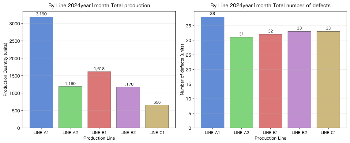
Data overview graph saved: no_overview_line_stats.svg

No.001: Understanding the Basics of SELECT Statements

Meaning in Practice

SELECT statement is a basic command for retrieving data in SQL.
From the quality control database, you can find out which parts have the highest number of defects, or if you want to check this month’s inspection records in a list.
All such analyses start with SELECT sentences.

Examples of use in manufacturing:

Extract only Parts Name and Number of Defects from the test records and use them for monthly reporting.
Extracting records of specific lines to use as materials for quality meetings

Approach to Analysis and Modeling

SELECT Minimum sentence structure:

SELECT list by name1, list by name2, ...
FROM   Table Name;

SELECT: The columns you want to retrieve (if there are multiple entries, separate them with commas)
FROM: Data source table
SQL statements end with a semicolon (;), but in Python sqlite3, they can be omitted
SQL keywords (SELECT and FROM) work in both uppercase and lowercase letters,
By convention, writing in capital letter distinguishes between SQL keywords and column names

Check with Python

# No.001: Basics of SELECT Sentences
# Retrieve three columns: part name, shift, and number of defects.
sql = '''
SELECT part_name, shift, defect_qty
FROM   inspections
LIMIT  8
'''
q(conn, sql)

── SQL ─────────────────────────────────────────
  SELECT part_name, shift, defect_qty
  FROM   inspections
  LIMIT  8
───────────────────────────────────────────────
shape: (8, 3)
┌────────────────────┬───────┬────────────┐
│ part_name          ┆ shift ┆ defect_qty │
│ ---                ┆ ---   ┆ ---        │
│ str                ┆ str   ┆ i64        │
╞════════════════════╪═══════╪════════════╡
│ piston ring     ┆ early shift  ┆ 3          │
│ Crankshaft   ┆ early shift  ┆ 5          │
│ brake pad     ┆ early shift  ┆ 2          │
│ piston ring     ┆ late shift  ┆ 7          │
│ Crankshaft   ┆ late shift  ┆ 4          │
│ brake caliper ┆ early shift  ┆ 6          │
│ Alternator       ┆ nighttime  ┆ 8          │
│ brake pad     ┆ late shift  ┆ 4          │
└────────────────────┴───────┴────────────┘
↳ Obtained in 8 lines

shape: (8, 3)

part_name	shift	defect_qty
str	str	i64
”piston ring"	"early shift”	3
”Crankshaft"	"early shift”	5
”brake pad"	"early shift”	2
”piston ring"	"late shift”	7
”Crankshaft"	"late shift”	4
”brake caliper"	"early shift”	6
”Alternator"	"nighttime”	8
”brake pad"	"late shift”	4

Reading the results

SELECT part_name, shift, defect_qty The 3only the column specified in the set will be returned
(There are 10 columns in the table, but you can extract only the necessary columns.)
FROM inspections clearly indicates which table to retrieve from
LIMIT 8 is a modifier to limit the first 8 entries (covered in detail in No.006).
The return order is in the order of insertion (id=1, 2, 3 … In that order,
This is If you want to guarantee sorting, ORDER BY necessary (Learn in No.007)

No.002: Specifying a table with a FROM clause

Meaning in Practice

FROM Specify “Which table to retrieve data from?” for the phrase.
Manufacturing databases typically contain multiple tables coexisting.

inspections (Inspection Record Table): Actual data such as date, line, number of defects, etc.
parts_master (Parts Master Table): Part code, name, category, unit price

By specifying the appropriate table name after the FROM according to the purpose,
Even with the same SELECT syntax, you can retrieve completely different data.

Approach to Analysis and Modeling

-- Retrieved from the inspection record table
SELECT ...
FROM   inspections;

-- Retrieved from the component master table (FROM Just change the phrase.)
SELECT ...
FROM   parts_master;

The table name following FROM is Case-sensitive. (according to the DB engine).
SQLite is case-insensitive, but for readability, uniform notation is recommended.

You can check the list of tables in the database in SQLite as follows:
SELECT name FROM sqlite_master WHERE type='table';

Check with Python

# No.002: FROM Phrases — Using Different Tables

# (1) Retrieve from the inspection record table
print('=== inspections Retrieve from the table ===')
sql1 = '''
SELECT part_code, part_name, production_qty, defect_qty
FROM   inspections
LIMIT  5
'''
q(conn, sql1)

print()

# (2) Retrieve from the component master table (just change the FROM clause)
print('=== parts_master Retrieve from the table ===')
sql2 = '''
SELECT part_code, part_name, category, unit_price, supplier
FROM   parts_master
'''
q(conn, sql2)

=== Retrieved from inspections table ===
── SQL ─────────────────────────────────────────
  SELECT part_code, part_name, production_qty, defect_qty
  FROM   inspections
  LIMIT  5
───────────────────────────────────────────────
shape: (5, 4)
┌───────────┬──────────────────┬────────────────┬────────────┐
│ part_code ┆ part_name        ┆ production_qty ┆ defect_qty │
│ ---       ┆ ---              ┆ ---            ┆ ---        │
│ str       ┆ str              ┆ i64            ┆ i64        │
╞═══════════╪══════════════════╪════════════════╪════════════╡
│ ENG-001   ┆ piston ring   ┆ 450            ┆ 3          │
│ ENG-002   ┆ Crankshaft ┆ 220            ┆ 5          │
│ BRK-001   ┆ brake pad   ┆ 380            ┆ 2          │
│ ENG-001   ┆ piston ring   ┆ 460            ┆ 7          │
│ ENG-002   ┆ Crankshaft ┆ 215            ┆ 4          │
└───────────┴──────────────────┴────────────────┴────────────┘
↳ Obtained in 5 rows

=== parts_master Get from Table ===
── SQL ─────────────────────────────────────────
  SELECT part_code, part_name, category, unit_price, supplier
  FROM   parts_master
───────────────────────────────────────────────
shape: (7, 5)
┌───────────┬────────────────────┬────────────────┬────────────┬──────────────┐
│ part_code ┆ part_name          ┆ category       ┆ unit_price ┆ supplier     │
│ ---       ┆ ---                ┆ ---            ┆ ---        ┆ ---          │
│ str       ┆ str                ┆ str            ┆ i64        ┆ str          │
╞═══════════╪════════════════════╪════════════════╪════════════╪══════════════╡
│ ENG-001   ┆ piston ring     ┆ Engine parts   ┆ 1200       ┆ Toyota Seiko   │
│ ENG-002   ┆ Crankshaft   ┆ Engine parts   ┆ 8500       ┆ Toyota Seiko   │
│ BRK-001   ┆ brake pad     ┆ brake parts   ┆ 950        ┆ Sumitomo Brake │
│ BRK-002   ┆ brake caliper ┆ brake parts   ┆ 4200       ┆ Sumitomo Brake │
│ ELC-001   ┆ Alternator       ┆ electrical components       ┆ 6800       ┆ Denso     │
│ ELC-002   ┆ Starter motor     ┆ electrical components       ┆ 3500       ┆ Denso     │
│ SUS-001   ┆ shock absorber ┆ suspension ┆ 2800       ┆ KYB          │
└───────────┴────────────────────┴────────────────┴────────────┴──────────────┘
↳ Obtained in 7 rows

shape: (7, 5)

part_code	part_name	category	unit_price	supplier
str	str	str	i64	str
”ENG-001"	"piston ring"	"Engine parts”	1200	”Toyota Seiko"
"ENG-002"	"Crankshaft"	"Engine parts”	8500	”Toyota Seiko"
"BRK-001"	"brake pad"	"brake parts”	950	”Sumitomo Brake"
"BRK-002"	"brake caliper"	"brake parts”	4200	”Sumitomo Brake"
"ELC-001"	"Alternator"	"electrical components”	6800	”Denso"
"ELC-002"	"Starter motor"	"electrical components”	3500	”Denso"
"SUS-001"	"shock absorber"	"suspension”	2800	”KYB”

Reading the results

FROM inspections: Inspection performance data (30 items) will be returned
→ A table storing actual values from the site, such as dates, lines, and defect counts.
FROM parts_master: Seven types of parts masters are returned
→ A table storing attribute information of parts (category, unit price, supplier)
Even with the same column name SELECT part_code, part_name, the information obtained varies depending on the FROM
In practice, you can use an achievement table like inspections as a ‘fact table’,
parts_master Attribute tables like those are called “Master Table (Dimension Table)“
The JOIN that binds the two is taught in Chapter 5 (No.041–050)

No.003: Retrieve All Columns

Meaning in Practice

SELECT * * (asterisk) is a wildcard meaning “All columns.”
If you’re unsure how many rows are on a table,
It’s convenient if you want to quickly check the contents of a new table.

Examples of use in manufacturing:

After data migration, check whether all rows in the table are correctly included
Understanding the structure of tables you encounter for the first time (exploratory analysis)

Approach to Analysis and Modeling

SELECT * is convenient, but there are two reasons to In the actual environment, it should generally be avoided. it.

Performance: Loads unnecessary columns, causing slowdowns in tables with large data volumes
Readability and Maintainability: When columns increase or decrease, query behavior changes, causing bugs in downstream processing.

The exploration and verification phase generally involves SELECT * and Clearly specify the required columns for reporting and analysis queries.

Check with Python

# No.003: SELECT * — Get All Columns
# Combine LIMIT to check the top 5 items
sql = '''
SELECT *
FROM   inspections
LIMIT  5
'''
q(conn, sql)
print()

# Check the table structure (column name and type)
print('── Checking the table structure ──────────────────────────')
cursor = conn.execute('PRAGMA table_info(inspections)')
for row in cursor.fetchall():
    cid, name, dtype, notnull, default, pk = row
    print(f'  {cid+1:2d}. {name:20s}  {dtype:8s}  {"PRIMARY KEY" if pk else "NOT NULL" if notnull else ""}')

── SQL ─────────────────────────────────────────
  SELECT *
  FROM   inspections
  LIMIT  5
───────────────────────────────────────────────
shape: (5, 10)
┌─────┬──────────────┬───────────┬───────────┬───┬───────┬──────────────┬────────────┬─────────────┐
│ id  ┆ inspection_d ┆ line_code ┆ part_code ┆ … ┆ shift ┆ production_q ┆ defect_qty ┆ inspector_c │
│ --- ┆ ate          ┆ ---       ┆ ---       ┆   ┆ ---   ┆ ty           ┆ ---        ┆ ode         │
│ i64 ┆ ---          ┆ str       ┆ str       ┆   ┆ str   ┆ ---          ┆ i64        ┆ ---         │
│     ┆ str          ┆           ┆           ┆   ┆       ┆ i64          ┆            ┆ str         │
╞═════╪══════════════╪═══════════╪═══════════╪═══╪═══════╪══════════════╪════════════╪═════════════╡
│ 1   ┆ 2024-01-04   ┆ LINE-A1   ┆ ENG-001   ┆ … ┆ early shift  ┆ 450          ┆ 3          ┆ INS-001     │
│ 2   ┆ 2024-01-04   ┆ LINE-A2   ┆ ENG-002   ┆ … ┆ early shift  ┆ 220          ┆ 5          ┆ INS-002     │
│ 3   ┆ 2024-01-04   ┆ LINE-B1   ┆ BRK-001   ┆ … ┆ early shift  ┆ 380          ┆ 2          ┆ INS-003     │
│ 4   ┆ 2024-01-05   ┆ LINE-A1   ┆ ENG-001   ┆ … ┆ late shift  ┆ 460          ┆ 7          ┆ INS-001     │
│ 5   ┆ 2024-01-05   ┆ LINE-A2   ┆ ENG-002   ┆ … ┆ late shift  ┆ 215          ┆ 4          ┆ INS-002     │
└─────┴──────────────┴───────────┴───────────┴───┴───────┴──────────────┴────────────┴─────────────┘
↳ Obtained in 5 rows

── Checking the table structure ──────────────────────────
   1. id                    INTEGER   PRIMARY KEY
   2. inspection_date       TEXT      NOT NULL
   3. line_code             TEXT      NOT NULL
   4. part_code             TEXT      NOT NULL
   5. part_name             TEXT      NOT NULL
   6. category              TEXT      NOT NULL
   7. shift                 TEXT      NOT NULL
   8. production_qty        INTEGER   NOT NULL
   9. defect_qty            INTEGER   NOT NULL
  10. inspector_code        TEXT      NOT NULL

Reading the results

SELECT * inspections whole10columns of the table will be returned
When there are many lines, the Polars display spreads horizontally, making it harder to check
→ This is one of the reasons why you should narrow down the queue in live queries.
PRAGMA table_info(Table Name) is a SQLite-specific command,
You can check the table column names, data types, and constraints
(Standard SQL uses DESCRIBE Table Name and information_schema)
This time, the table has 10 rows
Instead of collecting all rows every time, you can narrow it down to 3 to 5 rows depending on your needs.
This makes it much easier to convey the intent of your query

No.004: Retrieve only the necessary columns

Meaning in Practice

SELECT By explicitly specifying the column name you want to retrieve, you can You can narrow down only the information you need..
In the monthly quality report in manufacturing, five columns of “inspection date, line, part name, production quantity, and defect count” are sufficient,
“Inspector codes” and “categories” are often unnecessary in reports.

There are three advantages to narrowing down the columns:

Reduction of data transfer volume (especially effective for large tables)
Clarifying the intent of the query (You can instantly see what data you want to collect)
Improved stability of subsequent processing (Even if columns are added to the table, the result does not change)

Approach to Analysis and Modeling

If you specify multiple columns, separate them with Comma (,）.
For readability, writing with columns aligned vertically is recommended:

SELECT inspection_date,
       line_code,
       part_name,
       production_qty,
       defect_qty
FROM   inspections;

Check with Python

# No.004: Retrieve only the necessary columns
# Extract 5 columns for the monthly quality report
sql = '''
SELECT inspection_date,
       line_code,
       part_name,
       production_qty,
       defect_qty
FROM   inspections
LIMIT  10
'''
q(conn, sql)

── SQL ─────────────────────────────────────────
  SELECT inspection_date,
         line_code,
         part_name,
         production_qty,
         defect_qty
  FROM   inspections
  LIMIT  10
───────────────────────────────────────────────
shape: (10, 5)
┌─────────────────┬───────────┬────────────────────┬────────────────┬────────────┐
│ inspection_date ┆ line_code ┆ part_name          ┆ production_qty ┆ defect_qty │
│ ---             ┆ ---       ┆ ---                ┆ ---            ┆ ---        │
│ str             ┆ str       ┆ str                ┆ i64            ┆ i64        │
╞═════════════════╪═══════════╪════════════════════╪════════════════╪════════════╡
│ 2024-01-04      ┆ LINE-A1   ┆ piston ring     ┆ 450            ┆ 3          │
│ 2024-01-04      ┆ LINE-A2   ┆ Crankshaft   ┆ 220            ┆ 5          │
│ 2024-01-04      ┆ LINE-B1   ┆ brake pad     ┆ 380            ┆ 2          │
│ 2024-01-05      ┆ LINE-A1   ┆ piston ring     ┆ 460            ┆ 7          │
│ 2024-01-05      ┆ LINE-A2   ┆ Crankshaft   ┆ 215            ┆ 4          │
│ 2024-01-05      ┆ LINE-B2   ┆ brake caliper ┆ 180            ┆ 6          │
│ 2024-01-08      ┆ LINE-C1   ┆ Alternator       ┆ 120            ┆ 8          │
│ 2024-01-08      ┆ LINE-B1   ┆ brake pad     ┆ 390            ┆ 4          │
│ 2024-01-09      ┆ LINE-A1   ┆ piston ring     ┆ 470            ┆ 2          │
│ 2024-01-09      ┆ LINE-C1   ┆ Starter motor     ┆ 100            ┆ 3          │
└─────────────────┴───────────┴────────────────────┴────────────────┴────────────┘
↳ Obtained in 10 lines

shape: (10, 5)

inspection_date	line_code	part_name	production_qty	defect_qty
str	str	str	i64	i64
”2024-01-04"	"LINE-A1"	"piston ring”	450	3
”2024-01-04"	"LINE-A2"	"Crankshaft”	220	5
”2024-01-04"	"LINE-B1"	"brake pad”	380	2
”2024-01-05"	"LINE-A1"	"piston ring”	460	7
”2024-01-05"	"LINE-A2"	"Crankshaft”	215	4
”2024-01-05"	"LINE-B2"	"brake caliper”	180	6
”2024-01-08"	"LINE-C1"	"Alternator”	120	8
”2024-01-08"	"LINE-B1"	"brake pad”	390	4
”2024-01-09"	"LINE-A1"	"piston ring”	470	2
”2024-01-09"	"LINE-C1"	"Starter motor”	100	3

Reading the results

The table has been narrowed down from 10 columns in SELECT * to 5columns, making the table significantly easier to read
Unnecessary category, shift, inspector_code, etc. are excluded from the report
By placing production_qty (number of production) and defect_qty (number of defects) side by side,
You can intuitively identify “excellent lines with high production volume but few defects.”
In practice, these five columns are exported to Excel and used as the basis for reports
By formatting this much in SQL, you can minimize the work done in Excel

No.005: Giving Columns Another Name

Meaning in Practice

Using AS keywords, you can assign Alias to the retrieved columns.
It is used to display English column names in Japanese or to give formulas easy-to-understand names.

Examples of use in manufacturing:

defect_qty → defective count displayed and pasted into Excel
defect_qty * 1.0 / production_qty * 100 → defect rate(%) Name it
inspection_date → Examination Date to create reports for those in charge

Approach to Analysis and Modeling

AS syntax:

SELECT Original Column Name AS Alias, ...
FROM   Table Name;

AS can be omitted, but since skipping them makes it easier to overlook, it is AS It is recommended to clearly indicate this.
When using space or Japanese as aliases, depending on the database engine, you may need to enclose them in quotation marks
In SQLite, you can use the Japanese aliases as they are (for reliability, enclosing them in double quotes)
Alias can be referenced in ORDER BY, but not in WHERE clauses
(This is a matter of execution order.) Details will be explained in No.010)

Check with Python

# No.005: Giving Columns Another Name
# Display English column names in Japanese and assign names to the calculation sequences
sql = '''
SELECT inspection_date    AS "Examination Date",
       line_code           AS "Line",
       part_name           AS "Part Name",
       production_qty      AS "Production Volume",
       defect_qty          AS "defective_count",
       ROUND(defect_qty * 100.0 / production_qty, 2) AS "defect_rate"
FROM   inspections
LIMIT  8
'''
q(conn, sql)

── SQL ─────────────────────────────────────────
  SELECT inspection_date AS inspection date,
         line_code AS line,
         part_name Name of the AS part,
         production_qty AS production volume,
         defect_qty Number of defective AS,
         ROUND(defect_qty * 100.0 / production_qty, 2) AS Defect Rate
  FROM   inspections
  LIMIT  8
───────────────────────────────────────────────
shape: (8, 6)
┌────────────┬─────────┬────────────────────┬────────┬────────┬────────┐
│ Examination Date     ┆ Line  ┆ Part Name             ┆ Production Volume ┆ defective_count ┆ defect_rate │
│ ---        ┆ ---     ┆ ---                ┆ ---    ┆ ---    ┆ ---    │
│ str        ┆ str     ┆ str                ┆ i64    ┆ i64    ┆ f64    │
╞════════════╪═════════╪════════════════════╪════════╪════════╪════════╡
│ 2024-01-04 ┆ LINE-A1 ┆ piston ring     ┆ 450    ┆ 3      ┆ 0.67   │
│ 2024-01-04 ┆ LINE-A2 ┆ Crankshaft   ┆ 220    ┆ 5      ┆ 2.27   │
│ 2024-01-04 ┆ LINE-B1 ┆ brake pad     ┆ 380    ┆ 2      ┆ 0.53   │
│ 2024-01-05 ┆ LINE-A1 ┆ piston ring     ┆ 460    ┆ 7      ┆ 1.52   │
│ 2024-01-05 ┆ LINE-A2 ┆ Crankshaft   ┆ 215    ┆ 4      ┆ 1.86   │
│ 2024-01-05 ┆ LINE-B2 ┆ brake caliper ┆ 180    ┆ 6      ┆ 3.33   │
│ 2024-01-08 ┆ LINE-C1 ┆ Alternator       ┆ 120    ┆ 8      ┆ 6.67   │
│ 2024-01-08 ┆ LINE-B1 ┆ brake pad     ┆ 390    ┆ 4      ┆ 1.03   │
└────────────┴─────────┴────────────────────┴────────┴────────┴────────┘
↳ Obtained in 8 lines

shape: (8, 6)

Examination Date	Line	Part Name	Production Volume	defective_count	defect_rate
str	str	str	i64	i64	f64
”2024-01-04"	"LINE-A1"	"piston ring”	450	3	0.67
”2024-01-04"	"LINE-A2"	"Crankshaft”	220	5	2.27
”2024-01-04"	"LINE-B1"	"brake pad”	380	2	0.53
”2024-01-05"	"LINE-A1"	"piston ring”	460	7	1.52
”2024-01-05"	"LINE-A2"	"Crankshaft”	215	4	1.86
”2024-01-05"	"LINE-B2"	"brake caliper”	180	6	3.33
”2024-01-08"	"LINE-C1"	"Alternator”	120	8	6.67
”2024-01-08"	"LINE-B1"	"brake pad”	390	4	1.03

Reading the results

The column header changed to Japanese and became Easy-to-Read Tables for Staff
ROUND(defect_qty * 100.0 / production_qty, 2) AS defect rate is
The formula (defect rate = number of defects ÷ number of productions × 100) is given the easy-to-understand name defect rate
ROUND(..., 2) is a function that rounds to two decimal places.
defect_qty * 100.0 / production_qty 100.0 (floating point) is important
100 (integers) may result in integer division,
For decimal point calculations, 1.0 and 100.0 use is safer.
If you save SQL with a “Japanese heading + calculation column” like this,
You can retrieve data in the same format every month

No.006: Limit the number of items you can obtain

Meaning in Practice

LIMIT By using clauses, you can specify the maximum number of lines to retrieve.
In manufacturing databases, inspection records can range from tens of thousands to hundreds of thousands,
If you collect all items, processing becomes sluggish.

Typical use in practice:

Data Verification: LIMIT 5 Look at only the first five listings and quickly grasp the column content.
Sample Acquisition: Extract sample data in LIMIT 100 and check statistics in Python
Ranking display: Top 10 defects in ORDER BY defect_qty DESC LIMIT 10

Approach to Analysis and Modeling

SELECT ...
FROM   Table Name
LIMIT  number of cases;          -- Lead N records

Differences in syntax by database engine:

DB	syntax
SQLite, MySQL, PostgreSQL	`LIMIT n`
SQL Server	`SELECT TOP n ...`
Oracle, Standard SQL	`FETCH FIRST n ROWS ONLY`

In this course, we use LIMIT to use SQLite.

Check with Python

# No.006: Limit the number of items you can obtain

# (1) LIMIT 3: Check only the first three items
print('=== LIMIT 3 ===')
sql1 = '''
SELECT id, inspection_date, line_code, part_name, defect_qty
FROM   inspections
LIMIT  3
'''
q(conn, sql1)
print()

# (2) LIMIT 10: First 10 items
print('=== LIMIT 10 ===')
sql2 = '''
SELECT id, inspection_date, line_code, part_name, defect_qty
FROM   inspections
LIMIT  10
'''
q(conn, sql2)
print()

# (3) No LIMIT: All items obtained (only the number of cases confirmed)
total = conn.execute('SELECT COUNT(*) FROM inspections').fetchone()[0]
print(f'LIMIT None (all items): {total} records')

=== LIMIT 3 ===
── SQL ─────────────────────────────────────────
  SELECT id, inspection_date, line_code, part_name, defect_qty
  FROM   inspections
  LIMIT  3
───────────────────────────────────────────────
shape: (3, 5)
┌─────┬─────────────────┬───────────┬──────────────────┬────────────┐
│ id  ┆ inspection_date ┆ line_code ┆ part_name        ┆ defect_qty │
│ --- ┆ ---             ┆ ---       ┆ ---              ┆ ---        │
│ i64 ┆ str             ┆ str       ┆ str              ┆ i64        │
╞═════╪═════════════════╪═══════════╪══════════════════╪════════════╡
│ 1   ┆ 2024-01-04      ┆ LINE-A1   ┆ piston ring   ┆ 3          │
│ 2   ┆ 2024-01-04      ┆ LINE-A2   ┆ Crankshaft ┆ 5          │
│ 3   ┆ 2024-01-04      ┆ LINE-B1   ┆ brake pad   ┆ 2          │
└─────┴─────────────────┴───────────┴──────────────────┴────────────┘
↳ Retrieved in 3 lines

=== LIMIT 10 ===
── SQL ─────────────────────────────────────────
  SELECT id, inspection_date, line_code, part_name, defect_qty
  FROM   inspections
  LIMIT  10
───────────────────────────────────────────────
shape: (10, 5)
┌─────┬─────────────────┬───────────┬────────────────────┬────────────┐
│ id  ┆ inspection_date ┆ line_code ┆ part_name          ┆ defect_qty │
│ --- ┆ ---             ┆ ---       ┆ ---                ┆ ---        │
│ i64 ┆ str             ┆ str       ┆ str                ┆ i64        │
╞═════╪═════════════════╪═══════════╪════════════════════╪════════════╡
│ 1   ┆ 2024-01-04      ┆ LINE-A1   ┆ piston ring     ┆ 3          │
│ 2   ┆ 2024-01-04      ┆ LINE-A2   ┆ Crankshaft   ┆ 5          │
│ 3   ┆ 2024-01-04      ┆ LINE-B1   ┆ brake pad     ┆ 2          │
│ 4   ┆ 2024-01-05      ┆ LINE-A1   ┆ piston ring     ┆ 7          │
│ 5   ┆ 2024-01-05      ┆ LINE-A2   ┆ Crankshaft   ┆ 4          │
│ 6   ┆ 2024-01-05      ┆ LINE-B2   ┆ brake caliper ┆ 6          │
│ 7   ┆ 2024-01-08      ┆ LINE-C1   ┆ Alternator       ┆ 8          │
│ 8   ┆ 2024-01-08      ┆ LINE-B1   ┆ brake pad     ┆ 4          │
│ 9   ┆ 2024-01-09      ┆ LINE-A1   ┆ piston ring     ┆ 2          │
│ 10  ┆ 2024-01-09      ┆ LINE-C1   ┆ Starter motor     ┆ 3          │
└─────┴─────────────────┴───────────┴────────────────────┴────────────┘
↳ Obtained in 10 lines

No LIMIT (all items): 30 items

Reading the results

LIMIT 3 returns the top 3 results, and LIMIT 10 returns the top 10 entries
LIMIT If there is no such thing, the entire table30The case will be retrieved
If you SELECT without LIMIT when there are tens of thousands of production tables, the system load increases
COUNT(*) is a counting function for counting the number of cases (learn more in Chapter 3, No.021)
Here, I use it as a function to check the total number of items
Combining LIMIT and ORDER BY results in ‘Worst N listings’ and ‘Top N listings’
Efficiently obtain (used in combination with No.007/008)

No.007: Sort by ORDER BY

Meaning in Practice

Using ORDER BY clauses, records can be sorted in Order of values in the specified column.
In quality control, we want to display the line with the highest number of defects at the beginning, or check in order of oldest inspection date.
Situations like this happen frequently.

Examples of use in manufacturing:

ORDER BY defect_qty → Ranked in order of least defects (in order of promotion)
ORDER BY inspection_date → Check in chronological order from oldest test date
ORDER BY line_code, inspection_date → Organized by line and date

Approach to Analysis and Modeling

ORDER BY syntax:

SELECT ...
FROM   Table Name
ORDER BY list by name;     -- The default is ascending order (the smallest value comes first).

The default is Seung-soon (ASC: Ascending） — numbers are in ascending order, strings are in alphabetical order
If you want to use descending order, add DESC (covered in detail in No.008).
Rearrange in multiple rows: ORDER BY columns1, columns2 — Arrange in column 1; if equipped, arrange in column 2
ORDER BY is written after WHERE and GROUP BY,
The execution order is immediately after SELECT (explained in No.010).

Check with Python

# No.007: ORDER BY — Sort in ascending order of defects (from smallest to lowest)
sql = '''
SELECT inspection_date AS "Examination Date",
       line_code        AS "Line",
       part_name        AS "Part Name",
       defect_qty       AS "defective_count"
FROM   inspections
ORDER BY defect_qty
LIMIT  10
'''
q(conn, sql)

── SQL ─────────────────────────────────────────
  SELECT inspection_date AS inspection date,
         line_code AS line,
         part_name Name of the AS part,
         defect_qty Number of After-Sales Service Defects
  FROM   inspections
  ORDER BY defect_qty
  LIMIT  10
───────────────────────────────────────────────
shape: (10, 4)
┌────────────┬─────────┬──────────────────┬────────┐
│ Examination Date     ┆ Line  ┆ Part Name           ┆ defective_count │
│ ---        ┆ ---     ┆ ---              ┆ ---    │
│ str        ┆ str     ┆ str              ┆ i64    │
╞════════════╪═════════╪══════════════════╪════════╡
│ 2024-01-04 ┆ LINE-B1 ┆ brake pad   ┆ 2      │
│ 2024-01-09 ┆ LINE-A1 ┆ piston ring   ┆ 2      │
│ 2024-01-22 ┆ LINE-A1 ┆ piston ring   ┆ 2      │
│ 2024-01-23 ┆ LINE-B2 ┆ brake pad   ┆ 2      │
│ 2024-01-04 ┆ LINE-A1 ┆ piston ring   ┆ 3      │
│ 2024-01-09 ┆ LINE-C1 ┆ Starter motor   ┆ 3      │
│ 2024-01-15 ┆ LINE-A2 ┆ Crankshaft ┆ 3      │
│ 2024-01-17 ┆ LINE-B1 ┆ brake pad   ┆ 3      │
│ 2024-01-05 ┆ LINE-A2 ┆ Crankshaft ┆ 4      │
│ 2024-01-08 ┆ LINE-B1 ┆ brake pad   ┆ 4      │
└────────────┴─────────┴──────────────────┴────────┘
↳ Obtained in 10 lines

shape: (10, 4)

Examination Date	Line	Part Name	defective_count
str	str	str	i64
”2024-01-04"	"LINE-B1"	"brake pad”	2
”2024-01-09"	"LINE-A1"	"piston ring”	2
”2024-01-22"	"LINE-A1"	"piston ring”	2
”2024-01-23"	"LINE-B2"	"brake pad”	2
”2024-01-04"	"LINE-A1"	"piston ring”	3
”2024-01-09"	"LINE-C1"	"Starter motor”	3
”2024-01-15"	"LINE-A2"	"Crankshaft”	3
”2024-01-17"	"LINE-B1"	"brake pad”	3
”2024-01-05"	"LINE-A2"	"Crankshaft”	4
”2024-01-08"	"LINE-B1"	"brake pad”	4

Reading the results

ORDER BY defect_qty is sorted to Sorted by number of defects (in order of promotion)
The default sorting direction is ascending (ASC)
Multiple records with 2 defects are displayed at the top
It is important to note that the order within the same number of defective records is not guaranteed
→ Including the date, setting ORDER BY defect_qty, inspection_date stabilizes the order
Because you can instantly identify the lines and parts with the fewest defects,
It can be used for analyzing “deploying best practices from excellent lines horizontally to other lines.”

No.008: Specify ascending or descending order

Meaning in Practice

By adding ASC (ascending) or DESC (descending) after ORDER BY,
You can explicitly specify the direction of sorting.

Differentiation in manufacturing:

ORDER BY defect_qty DESC → Ranked by Worst Number of Defects (Identifying the Problem Line)
ORDER BY defect_qty ASC → Ranked by Number of Defects (Identifying Model Improvement Lines)
Check from ORDER BY inspection_date DESC → Latest inspection records

Approach to Analysis and Modeling

ORDER BY list by name ASC   -- Ascending order (default): small → big
ORDER BY list by name DESC  -- descending order:               big → small

Multi-column combinations:

ORDER BY line_code ASC, defect_qty DESC

→ First, arrange them in ascending order by line chords, and within the same line, arrange them in order of the number of defects.
This allows you to list the “worst records by line.”

Check with Python

# No.008: Distinguishing between descending and ascending order

# (1) Descending Order (DESC): Ranked by the worst number of defects
print('=== ORDER BY defect_qty DESC(Worst order) ===')
sql_desc = '''
SELECT inspection_date AS "Examination Date",
       line_code        AS "Line",
       part_name        AS "Part Name",
       shift            AS "Shift",
       defect_qty       AS "defective_count"
FROM   inspections
ORDER BY defect_qty DESC
LIMIT  8
'''
q(conn, sql_desc)
print()

# (2) Composite ORDER BY: line ascending order + defect count descending order
print('=== ORDER BY line_code ASC, defect_qty DESC(Worst by line) ===')
sql_combo = '''
SELECT line_code  AS "Line",
       part_name  AS "Part Name",
       shift      AS "Shift",
       defect_qty AS "defective_count"
FROM   inspections
ORDER BY line_code ASC, defect_qty DESC
LIMIT  10
'''
q(conn, sql_combo)
print()

# (3) Bar Graph: Visualizing ORDER BY DESC Results
rows = conn.execute('''
    SELECT line_code || '-' || part_code AS label,
           defect_qty
    FROM   inspections
    ORDER BY defect_qty DESC
    LIMIT  10
''').fetchall()
labels = [r[0] for r in rows]
values = [r[1] for r in rows]

fig, ax = plt.subplots(figsize=(10, 5))
colors = ['#D65F5F' if v >= 10 else '#4878CF' for v in values]
bars = ax.barh(list(reversed(labels)), list(reversed(values)),
               color=list(reversed(colors)), alpha=0.85, edgecolor='black', linewidth=0.4)
for bar in bars:
    ax.text(bar.get_width() + 0.1, bar.get_y() + bar.get_height()/2,
            f'{int(bar.get_width())}', va='center', fontsize=9)
ax.set_title('ORDER BY defect_qty DESC — "Worst defect count"10"(Line"×"Parts)"', fontsize=12, pad=10)
ax.set_xlabel('Number of defects (units)', fontsize=10)
ax.set_ylabel('Line-Part code', fontsize=10)
ax.grid(axis='x', alpha=0.3)
ax.axvline(x=10, color='#D65F5F', linestyle='--', linewidth=1, alpha=0.6, label='defective_count=10 threshold')
ax.legend(fontsize=9)
plt.tight_layout()
plt.savefig('no008_order_by_desc.svg', format='svg', bbox_inches='tight')
plt.show()
print('Saved: no008_order_by_desc.svg')

=== ORDER BY defect_qty DESC (in order of worst) ===
── SQL ─────────────────────────────────────────
  SELECT inspection_date AS inspection date,
         line_code AS line,
         part_name Name of the AS part,
         shift AS,
         defect_qty Number of After-Sales Service Defects
  FROM   inspections
  ORDER BY defect_qty DESC
  LIMIT  8
───────────────────────────────────────────────
shape: (8, 5)
┌────────────┬─────────┬────────────────────┬────────┬────────┐
│ Examination Date     ┆ Line  ┆ Part Name             ┆ Shift ┆ defective_count │
│ ---        ┆ ---     ┆ ---                ┆ ---    ┆ ---    │
│ str        ┆ str     ┆ str                ┆ str    ┆ i64    │
╞════════════╪═════════╪════════════════════╪════════╪════════╡
│ 2024-01-16 ┆ LINE-A1 ┆ piston ring     ┆ nighttime   ┆ 15     │
│ 2024-01-11 ┆ LINE-B1 ┆ brake pad     ┆ nighttime   ┆ 12     │
│ 2024-01-22 ┆ LINE-B1 ┆ shock absorber ┆ late shift   ┆ 11     │
│ 2024-01-10 ┆ LINE-A2 ┆ shock absorber ┆ late shift   ┆ 9      │
│ 2024-01-18 ┆ LINE-B2 ┆ brake caliper ┆ nighttime   ┆ 9      │
│ 2024-01-08 ┆ LINE-C1 ┆ Alternator       ┆ nighttime   ┆ 8      │
│ 2024-01-05 ┆ LINE-A1 ┆ piston ring     ┆ late shift   ┆ 7      │
│ 2024-01-15 ┆ LINE-B2 ┆ shock absorber ┆ late shift   ┆ 7      │
└────────────┴─────────┴────────────────────┴────────┴────────┘
↳ Obtained in 8 lines

=== ORDER BY line_code ASC, defect_qty DESC (Worst by Line) ===
── SQL ─────────────────────────────────────────
  SELECT line_code AS line,
         part_name Name of the AS part,
         shift AS,
         defect_qty Number of After-Sales Service Defects
  FROM   inspections
  ORDER BY line_code ASC, defect_qty DESC
  LIMIT  10
───────────────────────────────────────────────
shape: (10, 4)
┌─────────┬────────────────────┬────────┬────────┐
│ Line  ┆ Part Name             ┆ Shift ┆ defective_count │
│ ---     ┆ ---                ┆ ---    ┆ ---    │
│ str     ┆ str                ┆ str    ┆ i64    │
╞═════════╪════════════════════╪════════╪════════╡
│ LINE-A1 ┆ piston ring     ┆ nighttime   ┆ 15     │
│ LINE-A1 ┆ piston ring     ┆ late shift   ┆ 7      │
│ LINE-A1 ┆ piston ring     ┆ late shift   ┆ 5      │
│ LINE-A1 ┆ piston ring     ┆ early shift   ┆ 4      │
│ LINE-A1 ┆ piston ring     ┆ early shift   ┆ 3      │
│ LINE-A1 ┆ piston ring     ┆ early shift   ┆ 2      │
│ LINE-A1 ┆ piston ring     ┆ early shift   ┆ 2      │
│ LINE-A2 ┆ shock absorber ┆ late shift   ┆ 9      │
│ LINE-A2 ┆ Crankshaft   ┆ early shift   ┆ 6      │
│ LINE-A2 ┆ Crankshaft   ┆ early shift   ┆ 5      │
└─────────┴────────────────────┴────────┴────────┘
↳ Obtained in 10 lines

svg

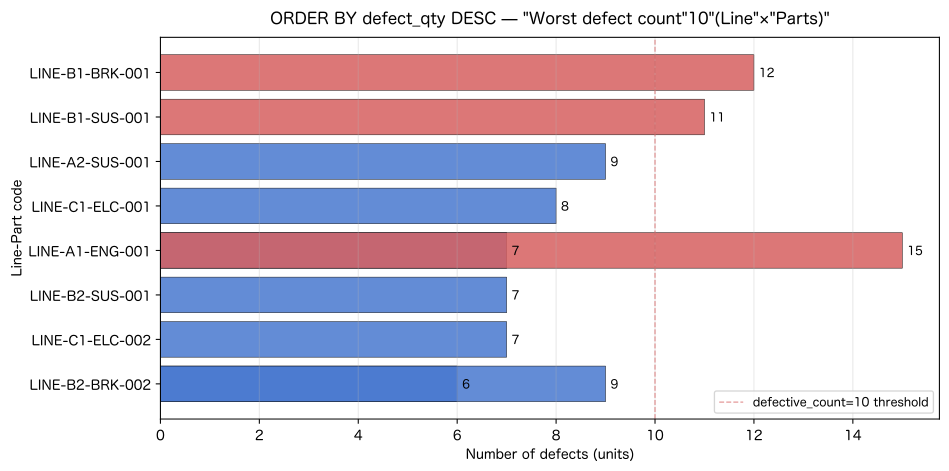
Saved: no008_order_by_desc.svg

Reading the results

DESC(descending order) are ranked in order of the number of defects, and the worst record is placed at the top
The highest number of defects is LINE-A1 / piston ring / nighttime, 15 — a key point to focus on during night shifts.
compound ORDER BY (line_code ASC, defect_qty DESC)
You can organize the worst records by line
→ It is clear that defects are concentrated in LINE-A1’s night shifts
Visualized the results of ORDER BY in Graph (Bar Graph)
The red bars (number of defects≥ 10) are concentrated in LINE-A1 and LINE-B1,
These are the lines that should be prioritized for improvement
In practice, the ‘monthly worst ranking’ is automatically retrieved every month using this SQL,
It can be used as material for quality meetings

No.009: Eliminating Duplicates in DISTINCT

Meaning in Practice

SELECT DISTINCT gets Only unique values, excluding duplicate values,.
In the manufacturing database, you can see how many types of parts are registered in this table.
It is often used to check “how many lines are being inspected.”

Examples of use in manufacturing:

SELECT DISTINCT part_code → Obtain a list of part codes subject to inspection
SELECT DISTINCT line_code → Check the list of operating lines
SELECT DISTINCT line_code, shift → Understanding the combination of line × shift

Approach to Analysis and Modeling

SELECT DISTINCT list by name
FROM   Table Name;

DISTINCT is placed immediately after SELECT
multi-row DISTINCT: In the case of SELECT DISTINCT columns1, columns2,
Only records with unique combinations of columns 1 and 2 are returned
DISTINCT loads all data and then removes duplicates,
Tables with many entries have higher computational costs

The set of unique values obtained from DISTINCT is
It can also be used for Master Table (parts_master etc.).
Check whether all part codes appearing in the inspection records are registered in the master.
This serves as a starting point for verification (covered in detail in Chapter 5, JOIN).

Check with Python

# No.009: DISTINCT — Retrieves only unique values excluding duplicates

# (1) Inspection Target Part Code (Duplicate Removal)
print('=== SELECT DISTINCT part_code ===')
sql1 = '''
SELECT DISTINCT part_code
FROM   inspections
ORDER BY part_code
'''
q(conn, sql1)
print()

# (2) List of lines (duplication removal)
print('=== SELECT DISTINCT line_code ===')
sql2 = '''
SELECT DISTINCT line_code
FROM   inspections
ORDER BY line_code
'''
q(conn, sql2)
print()

# (3) Combination of Line × Shift (Multiple Rows of DISTINCT)
print('=== SELECT DISTINCT line_code, shift ===')
sql3 = '''
SELECT DISTINCT line_code, shift
FROM   inspections
ORDER BY line_code, shift
'''
q(conn, sql3)
print()

# Comparison of the number of cases with or without DISTINCT
total    = conn.execute('SELECT COUNT(part_code) FROM inspections').fetchone()[0]
distinct = conn.execute('SELECT COUNT(DISTINCT part_code) FROM inspections').fetchone()[0]
print(f'part_code Total number of cases: {total} records → DISTINCT After: {distinct} records')

=== SELECT DISTINCT part_code ===
── SQL ─────────────────────────────────────────
  SELECT DISTINCT part_code
  FROM   inspections
  ORDER BY part_code
───────────────────────────────────────────────
shape: (7, 1)
┌───────────┐
│ part_code │
│ ---       │
│ str       │
╞═══════════╡
│ BRK-001   │
│ BRK-002   │
│ ELC-001   │
│ ELC-002   │
│ ENG-001   │
│ ENG-002   │
│ SUS-001   │
└───────────┘
↳ Obtained in 7 rows

=== SELECT DISTINCT line_code ===
── SQL ─────────────────────────────────────────
  SELECT DISTINCT line_code
  FROM   inspections
  ORDER BY line_code
───────────────────────────────────────────────
shape: (5, 1)
┌───────────┐
│ line_code │
│ ---       │
│ str       │
╞═══════════╡
│ LINE-A1   │
│ LINE-A2   │
│ LINE-B1   │
│ LINE-B2   │
│ LINE-C1   │
└───────────┘
↳ Obtained in 5 rows

=== SELECT DISTINCT line_code, shift ===
── SQL ─────────────────────────────────────────
  SELECT DISTINCT line_code, shift
  FROM   inspections
  ORDER BY line_code, shift
───────────────────────────────────────────────
shape: (14, 2)
┌───────────┬───────┐
│ line_code ┆ shift │
│ ---       ┆ ---   │
│ str       ┆ str   │
╞═══════════╪═══════╡
│ LINE-A1   ┆ nighttime  │
│ LINE-A1   ┆ early shift  │
│ LINE-A1   ┆ late shift  │
│ LINE-A2   ┆ early shift  │
│ LINE-A2   ┆ late shift  │
│ …         ┆ …     │
│ LINE-B2   ┆ early shift  │
│ LINE-B2   ┆ late shift  │
│ LINE-C1   ┆ nighttime  │
│ LINE-C1   ┆ early shift  │
│ LINE-C1   ┆ late shift  │
└───────────┴───────┘
↳ Retrieved in 14 rows

Total number of part_code cases: 30 → after DISTINCT: 7

Reading the results

You can check 7Part code for type in SELECT DISTINCT part_code
(Out of 30 inspection records, 7 parts codes = 7 rows in the table × multiple entries)
From the line list (DISTINCT line_code), you can see that 5Line is currently active
From the combination of DISTINCT line_code, shift,
You can check the shift configurations being made on each line
→ It can be seen that some lines are not implementing night shifts
COUNT(part_code) = 30 records (with overlaps), COUNT(DISTINCT part_code) = 7 cases
This difference shows the average of “how many times each part was inspected” (30÷7 ≈ 4.3 times per part)

No.010: Understanding the SQL execution order

Meaning in Practice

Many SQL bugs arise from “The difference between the order in which you write and the order in which you execute.”
For example, if you try to use an alias given in SELECT with WHERE, it results in an error.
Common mistakes for beginners can be prevented by understanding this execution sequence.

Approach to Analysis and Modeling

SQL of Writing order：

① SELECT   Part Name, defect rate      -- Columns to get
② FROM     inspections         -- Table specification
③ WHERE    defect rate >= 1.0        -- ← Error! (There is no defect rate yet.)
④ ORDER BY defect rate DESC
⑤ LIMIT    5

SQL Order of execution (DB engine processing order):

execution order	sentence	Processing Details
1	FROM	Loading the table
2	WHERE	line filter
3	GROUP BY	Group Aggregation
4	HAVING	Narrowing down aggregate results
5	SELECT	Column Calculation and Definition of Alias
6	ORDER BY	sort
7	LIMIT	Limit on Number of Cases

WHERE is executed before SELECT (step 5), so
Alias defined in SELECT cannot be used in WHERE.
On the other hand, ORDER BY comes after SELECT, so you can refer to the alternative name of SELECT.

Check with Python

# No.010: Understanding the Execution Order

# (1) Use the alias SELECT for ORDER BY (OK — ORDER BY executes after SELECT)
print('=== SELECT Also known as ORDER BY used in (OK） ===')
sql_ok = '''
SELECT part_name                                    AS "Part Name",
       defect_qty * 100.0 / production_qty          AS "defect_rate",
       production_qty                               AS "Production Volume"
FROM   inspections
ORDER BY "defect_rate" DESC
LIMIT  5
'''
q(conn, sql_ok)
print()

# (2) Using an alias for SELECT in WHERE causes an error (WHERE is executed before SELECT)
print('=== SELECT Also known as WHERE Example of an error when used ===')
try:
    sql_ng = '''
    SELECT part_name AS "Part Name",
           defect_qty * 100.0 / production_qty AS "defect_rate"
    FROM   inspections
    WHERE  defect_rate >= 2.0
    '''
    conn.execute(sql_ng).fetchall()
except Exception as e:
    print(f'  error occurrence: {e}')
    print()
    print('  ↓ Correct Writing: WHERE Now, use the original formula')

# (3) Correct way to write: Use the original column name/formula in WHERE
print()
print('=== Correct Writing: WHERE Now, write the formula directly. ===')
sql_correct = '''
SELECT part_name                           AS "Part Name",
       defect_qty * 100.0 / production_qty AS "defect_rate",
       production_qty                      AS "Production Volume"
FROM   inspections
WHERE  defect_qty * 1.0 / production_qty >= 0.02
ORDER BY "defect_rate" DESC
'''
q(conn, sql_correct)

=== Use SELECT alias as ORDER BY (OK) ===
── SQL ─────────────────────────────────────────
  SELECT part_name AS Part Name,
         defect_qty * 100.0 / production_qty AS defect rate,
         production_qty After-Sales Service Production Volume
  FROM   inspections
  ORDER BY Defect Rate DESC
  LIMIT  5
───────────────────────────────────────────────
shape: (5, 3)
┌────────────────────┬──────────┬────────┐
│ Part Name             ┆ defect_rate   ┆ Production Volume │
│ ---                ┆ ---      ┆ ---    │
│ str                ┆ f64      ┆ i64    │
╞════════════════════╪══════════╪════════╡
│ shock absorber ┆ 12.5     ┆ 88     │
│ shock absorber ┆ 10.0     ┆ 90     │
│ shock absorber ┆ 8.235294 ┆ 85     │
│ Starter motor     ┆ 7.142857 ┆ 98     │
│ Alternator       ┆ 6.666667 ┆ 120    │
└────────────────────┴──────────┴────────┘
↳ Obtained in 5 rows

=== Example of an error when using SELECT alias in WHERE ===

=== Correct way to write: Write the formula directly in WHERE ===
── SQL ─────────────────────────────────────────
  SELECT part_name AS Part Name,
         defect_qty * 100.0 / production_qty AS defect rate,
         production_qty After-Sales Service Production Volume
  FROM   inspections
  WHERE  defect_qty * 1.0 / production_qty >= 0.02
  ORDER BY Defect Rate DESC
───────────────────────────────────────────────
shape: (17, 3)
┌────────────────────┬──────────┬────────┐
│ Part Name             ┆ defect_rate   ┆ Production Volume │
│ ---                ┆ ---      ┆ ---    │
│ str                ┆ f64      ┆ i64    │
╞════════════════════╪══════════╪════════╡
│ shock absorber ┆ 12.5     ┆ 88     │
│ shock absorber ┆ 10.0     ┆ 90     │
│ shock absorber ┆ 8.235294 ┆ 85     │
│ Starter motor     ┆ 7.142857 ┆ 98     │
│ Alternator       ┆ 6.666667 ┆ 120    │
│ …                  ┆ …        ┆ …      │
│ Starter motor     ┆ 3.0      ┆ 100    │
│ brake caliper ┆ 2.857143 ┆ 175    │
│ Crankshaft   ┆ 2.608696 ┆ 230    │
│ brake caliper ┆ 2.352941 ┆ 170    │
│ Crankshaft   ┆ 2.272727 ┆ 220    │
└────────────────────┴──────────┴────────┘
↳ Obtained in 17 rows

shape: (17, 3)

Part Name	defect_rate	Production Volume
str	f64	i64
”shock absorber”	12.5	88
”shock absorber”	10.0	90
”shock absorber”	8.235294	85
”Starter motor”	7.142857	98
”Alternator”	6.666667	120
…	…	…
”Starter motor”	3.0	100
”brake caliper”	2.857143	175
”Crankshaft”	2.608696	230
”brake caliper”	2.352941	170
”Crankshaft”	2.272727	220

# No.010: Diagram of SQL execution order (matplotlib)
fig, axes = plt.subplots(1, 2, figsize=(11, 7))

clauses_write = [
    ('① SELECT',   '#4878CF'),
    ('② FROM',     '#6ACC65'),
    ('③ WHERE',    '#D65F5F'),
    ('④ GROUP BY', '#B47CC7'),
    ('⑤ HAVING',   '#C4AD66'),
    ('⑥ ORDER BY', '#88BEAA'),
    ('⑦ LIMIT',    '#E07050'),
]
clauses_exec = [
    ('① FROM',     '#6ACC65'),
    ('② WHERE',    '#D65F5F'),
    ('③ GROUP BY', '#B47CC7'),
    ('④ HAVING',   '#C4AD66'),
    ('⑤ SELECT',   '#4878CF'),
    ('⑥ ORDER BY', '#88BEAA'),
    ('⑦ LIMIT',    '#E07050'),
]

titles = ['Writing order (SQL (Syntax)', 'The order in which they are executed (DB Engine)']
all_clauses = [clauses_write, clauses_exec]

for ax, title, clauses in zip(axes, titles, all_clauses):
    n = len(clauses)
    ax.set_xlim(0, 1)
    ax.set_ylim(-0.5, n - 0.5)
    ax.axis('off')
    ax.set_title(title, fontsize=12, fontweight='bold', pad=15)

    for i, (label, color) in enumerate(clauses):
        y = n - 1 - i
        ax.barh(y, 0.75, left=0.125, color=color, alpha=0.78, height=0.6,
                edgecolor='white', linewidth=1.5)
        ax.text(0.5, y, label, ha='center', va='center',
                fontsize=12, fontweight='bold', color='white')
        # Downward arrow (except for the last element)
        if i < n - 1:
            ax.annotate('', xy=(0.5, y - 0.38), xytext=(0.5, y - 0.32),
                        arrowprops=dict(arrowstyle='->', color='#555555', lw=1.5))

# Annotation that the order of SELECT and FROM is swapped.
axes[0].text(0.98, 6, '← SQL I start writing from here.', va='center', ha='right',
             fontsize=9, color='#4878CF', style='italic')
axes[1].text(0.98, 6, '← DB Start processing from here', va='center', ha='right',
             fontsize=9, color='#6ACC65', style='italic')
axes[1].text(0.98, 2, '← SELECT is first evaluated here', va='center', ha='right',
             fontsize=8, color='#4878CF', style='italic')

plt.suptitle('SQL The difference between the order in which you write and how you run it', fontsize=14, fontweight='bold', y=1.02)
plt.tight_layout()
plt.savefig('no010_sql_execution_order.svg', format='svg', bbox_inches='tight')
plt.show()
print('Saved: no010_sql_execution_order.svg')

findfont: Failed to find font weight bold, now using 400.


findfont: Failed to find font weight bold, now using 400.

svg

Saved: no010_sql_execution_order.svg

Reading the results

① OK Examples（ORDER BY defect rate DESC）:
You can define the alias defect rate in SELECT and then use it in ORDER BY
→ The execution order is 5 (SELECT) → 6 (ORDER BY), so you can refer to it
Records with defect rates of 2% or higher are displayed at the top as a result
② Examples of errors（WHERE defect rate >= 2.0）:
WHERE is processed in order 2, but the alias defect rate is defined in SELECT 5,
This results in an error saying “Such a column does not exist.”
→ WHERE Now, the original column names or Write the formula directly is the correct way to write it.
③ Correct Writing（WHERE defect_qty * 1.0 / production_qty >= 0.02）:
It works correctly by directly writing the formula within WHERE
Only records with a defect rate of 2% or higher (0.02) are filtered down and displayed in descending order
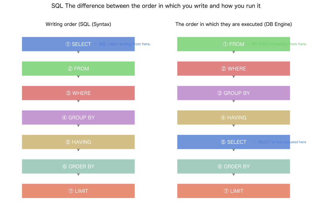
Diagram: When you arrange the writing and execution order, the positions of SELECT and FROM are swapped,
You can visually see that SELECT is actually rated fifth
Keeping this diagram in mind will help prevent SQL bugs in advance

Practical Implications Seen Through Target Exercise

Through Chapter 1 of No.001–010, the following insights can be gained for manufacturing data analysis.

1. SQL is the ‘primary tool’ for data analysis.

SQL is First Entrance in analyzing quality control data.
The tasks I used to do manually in Excel—sorting, narrowing columns, and removing duplicates—
With SQL, you can save and Every month0Reproduce in seconds the query as a re-executable one.

2. The habit of checking data using LIMIT before WHERE

When handling large volumes of data, first check the beginning in LIMIT 10,
It is important to have the habit of understanding the data type, presence or absence of NULL, and range of values before starting analysis.
If you accidentally run a large acquisition query in the production environment, it will affect the system.

3. Always clearly indicate ORDER BY

The assumption that “the order of the line will never change anyway” is dangerous.
When records are added or deleted from tables, or when the database version changes,
Queries without ORDER BY will be returned in a different order.
For reproducible analyses, ORDER BY Be sure to specify is the principle.

4. SELECT * is for search-only use; for report queries, the column is clearly specified.

SELECT * is dedicated to the exploration phase where you check what’s on the table.
Monthly quality reports, BI dashboards, and automation scripts include
Be sure to use Required columns clearly indicated SELECT.

5. Always be aware of the difference between the order in which you write and the order in which you execute

Many SQL bugs arise from “misunderstandings about execution order.”
FROM → WHERE → GROUP BY → HAVING → SELECT → ORDER BY → LIMIT
By keeping this execution order in mind, you can quickly identify the cause of the error.

What is necessary for practical implementation

Checklist for Implementing SQL for Data Analysis on the Manufacturing Floor

1. Database Environment Setup

Check the database engines used by the company’s quality management system (MySQL / Oracle / SQL Server / PostgreSQL, etc.)
SELECT Obtain a read-only account with permission (to prevent data destruction due to accidental operations)
Securely manage DB connection information (host, port, DB name, authentication credentials)

2. Understanding Data Structures

Check the column name, type, and constraint of the table you want to use in PRAGMA table_info or similar settings
Identify columns where NULL can fit and understand how to handle NULL (covered in Chapter 2, No.020)
Understand the relationships between tables (foreign keys) and prepare for JOIN (Chapter 5 No.041–050)

3. Query Management

Save frequently used queries as .sql files (using Git for version control is even better)
Record intent by adding a comment (-- Comments) to the query
Queries that require regular execution are automatically executed in Python using sqlite3 or sqlalchemy

4. Deployment to Quality Control Departments

Utilize this series (No.001–100) as internal SQL training textbooks
Establish queries for monthly quality reports so that all responsible staff can use them
Build a pipeline to visualize SQL results using matplotlib / Polars

Conclusion

In this chapter (No.001–010), we studied the basic SQL syntax using the inspection record database of an automotive parts manufacturer as the subject.

No.	What I learned	Practical Use
001	Basics of SELECT Statements	The first step in obtaining the first data from the database
002	Specifying tables with FROM clauses	Inspection Records / Switching Between Parts Masters
003	Get all rows with SELECT *	Quickly grasp the structure of new tables
004	Retrieve only the necessary columns	Minimize data for reporting
005	Give the column another name	Output English column names in Japanese and calculate column names
006	Limit the number of transactions with LIMIT	Sample N Samples of Large Volumes of Data
007	Sort by ORDER BY	Ranked by the number of defects from least to most
008	Specifying ascending and descending order	Instantly identify the Worst N and Best N Cases
009	Duplication with DISTINCT.	View part codes and line types at a glance
010	Understanding SQL execution order	Identifying the Cause of WHERE/ORDER BY Errors

Next chapter (Chapter 1)2Chapter: Setting Conditions and Filtering No.011〜020） So,
WHERE Learn to filter lines by phrases.
”Extract only lines with 10 or more defects” “View only records of specific lines”
You will master the core practical operations of these areas.

Consultations for Corporations

For DX promotion in manufacturing, building data analysis infrastructure, and in-house SQL/Python training,
Please feel free to consult with Suri Kobo.

📩 Contact Us: surikobo.co.jp/contact
Please feel free to consult us first.

This article is for “Data Analysis SQL Introduction 100The ‘Bookexercise’ series1This is the chapter.
The overall table of contents for the series is Here Please check from here.

Extracting and analyzing defective data from the inspection record database using SQL

Extracting and analyzing defective data from the inspection record database using SQL

SQL 100 Exercises Chapter 1 (No.001–No.010): SQL Basics

Introduction: Practical Challenges in Manufacturing Covered in This Article

Common situations on site

Why is this issue so difficult to judge?

1. The order in which you write and the order in which you execute are different

2. The Pitfalls of SELECT *

3. Return order without ORDER BY is not guaranteed

4. Handling NULL differs from intuition

Overview of Exercise covered this time

Preparing the Python environment

Creation of Fictional Data

No.001: Understanding the Basics of SELECT Statements

Meaning in Practice

Approach to Analysis and Modeling

Check with Python

Reading the results

No.002: Specifying a table with a FROM clause

Meaning in Practice

Approach to Analysis and Modeling

Check with Python

Reading the results

No.003: Retrieve All Columns

Meaning in Practice

Approach to Analysis and Modeling

Check with Python

Reading the results

No.004: Retrieve only the necessary columns

Meaning in Practice

Approach to Analysis and Modeling

Check with Python

Reading the results

No.005: Giving Columns Another Name

Meaning in Practice

Approach to Analysis and Modeling

Check with Python

Reading the results

No.006: Limit the number of items you can obtain

Meaning in Practice

Approach to Analysis and Modeling

Check with Python

Reading the results

No.007: Sort by ORDER BY

Meaning in Practice

Approach to Analysis and Modeling

Check with Python

Reading the results

No.008: Specify ascending or descending order

Meaning in Practice

Approach to Analysis and Modeling

Check with Python

Reading the results

No.009: Eliminating Duplicates in DISTINCT

Meaning in Practice

Approach to Analysis and Modeling

Check with Python

Reading the results

No.010: Understanding the SQL execution order

Meaning in Practice

Approach to Analysis and Modeling

Check with Python

Reading the results

Practical Implications Seen Through Target Exercise

1. SQL is the ‘primary tool’ for data analysis.

2. The habit of checking data using LIMIT before WHERE

3. Always clearly indicate ORDER BY

4. SELECT * is for search-only use; for report queries, the column is clearly specified.

5. Always be aware of the difference between the order in which you write and the order in which you execute

What is necessary for practical implementation

Checklist for Implementing SQL for Data Analysis on the Manufacturing Floor

1. Database Environment Setup

2. Understanding Data Structures

3. Query Management

4. Deployment to Quality Control Departments

Conclusion

Consultations for Corporations

Related Posts

Integrating data quality management, SQL design, and BI integration into production line operations

Deepening manufacturing decision-making with SQL application analysis techniques

2. The Pitfalls of `SELECT *`