Creating Production Plans Resilient to Fluctuations: 10 Exercises on Line Design and Capability Evaluation for Multi-Variety Parts Factories

In this article, we use a fictional precision parts factory as a subject and treat Line balancing, job shop, flow shop, scheduling, constraint formulation, simulation optimization, bottlenecks, takt time, production capacity, digital twin as a continuous process of decision-making.

Rather than just calculating individual methods, the goal is to explain with reproducible numbers “can we meet deadlines,” “where to allocate personnel and equipment,” and “how far we can withstand demand fluctuations.” The data you publish is generated in Python and does not depend on external data.

[!NOTE] This material is a notebook previously used by Surikoubo (or personally by the representative, Kazuyama), and has been reconstructed, edited, and published with the company’s permission.
All data listed is fictional and has no relation whatsoever to real companies, factories, or figures.

Introduction: Practical Challenges in Manufacturing Covered in This Article

The target is factories that machine, grind, and inspect multiple types before shipping. Order volumes change daily, and the process sequence and processing time differ by product type. Production managers must simultaneously assess not only daily assignments but also staffing, equipment expansion, work-in-progress inventory, and delivery deadline responses.

In this article, we divide decisions into “planned values” and “actual fluctuations.” First, load and sequence are calculated statically, then stops and processing time variations are incorporated into the simulation, and finally connected to a small prototype of the digital twin.

Common situations on site

• Even though the monthly plan was within my capacity, daily routines and arrangements caused delays in delivery.
• As a result of increasing the uptime rate of each process, the number of rigs before bottlenecks increases.
• Standard time is a single value, but results are scattered due to equipment stoppages, repairs, and differences in worker
• Deciding based solely on average values like “Should we add one more piece of equipment?” or “Can overtime absorb the benefits?”
• Even if you collect on-site results, there is no mechanism to return to the planning model, and the master becomes outdated.

These may seem like separate issues, but the common cause is that Process dependencies, finite capacity, and fluctuations is not viewed on the same scale.

Why is this issue so difficult to judge?

Even if the total production time is less than working hours, it does not guarantee meeting deadlines. If the previous process is not completed, the subsequent process cannot begin, and multiple jobs cannot use the same equipment simultaneously. Also, even with a high average capacity, if demand is below the lower end of the capacity distribution, shortages will occur.

Typical evaluation metrics include makespan, total latency, work-in-progress inventory, throughput, utilization rate, and demand fulfillment probability. Since maximizing a single KPI tends to lead to local optimization, the Delivery time, liquidity, cost, and robustness is included here.

Overview of Exercise covered this time

No.	Theme	Main Questions	Main Outputs
041	Line balancing	How many steps should the work be divided into	Process Load and Train Formation Efficiency
042	job shop	How to resolve conflicts in jobs across different routes	Gantt chart, completion time
043	Flow Shop	How to choose the order of entry for common routes	Shortest makespan
044	Scheduling	How to Distinguish Between Priority Delivery and Short Time Priority	Comparison of Delay Times
045	Formulation of constraints	Does the plan protect finite capabilities?	Restricting surplus capacity
046	Simulation optimization	Which personnel plan to choose amid fluctuations	Cost and Achievement Probability
047	Bottleneck Analysis	Where are the areas for improvement?	load rate, remaining power
048	takt time	How to determine the necessary pace based on demand	Tact and required number of people
049	Production capacity analysis	What percentage probability can demand be met?	Ability distribution and lower quantiles
050	Digital twin	How to update plans based on achievements	State estimation and scenario comparison

Preparing the Python environment

NumPy is used for numerical calculations, pandas for representing process and order data, and matplotlib for visualization. The random number generator is fixed to default_rng(42) so that the same results can be reproduced under the same conditions.

import itertools
import platform

import matplotlib.pyplot as plt
import numpy as np
import pandas as pd
import japanize_matplotlib
from IPython.display import display

SEED = 42
rng = np.random.default_rng(SEED)
pd.set_option("display.max_columns", 20)
pd.set_option("display.float_format", lambda x: f"{x:,.2f}")

print(f"Python: {platform.python_version()}")
print(f"NumPy: {np.__version__} / pandas: {pd.__version__}")
print(f"random numberseed: {SEED}")

Python: 3.13.1
NumPy: 2.5.1 / pandas: 3.0.3
Random seed: 42

Creation of Fictional Data

Imagine a factory that produces three products (A, B, C) through three processes: cutting, grinding, and inspection. Standard time refers to the net work per good product, and demand is per day. Additionally, we prepare assembly line elements and same-day order jobs.

In practice, it is important to define standard time (whether net time or including margin) and data granularity. To clarify the explanation, all units will be unified to ‘minute’.

products = pd.DataFrame({
    "Products": ["A", "B", "C"],
    "daily demand": [72, 48, 36],
    "cutting_minutes": [3.2, 4.5, 2.8],
    "grinding_minutes": [2.5, 3.0, 4.2],
    "inspection_minutes": [1.4, 1.8, 1.6],
}).set_index("Products")

assembly_tasks = pd.DataFrame({
    "assignment": ["Parts extraction", "press-in", "conclude", "application", "adjustment", "Power-On Inspection", "Visual inspection", "Packaging"],
    "standard_time_seconds": [28, 46, 38, 32, 55, 44, 29, 36],
})

orders = pd.DataFrame({
    "jobs": ["J1", "J2", "J3", "J4", "J5", "J6"],
    "processing_time_minutes": [80, 35, 55, 25, 65, 40],
    "delivery_time_minutes": [170, 100, 210, 85, 230, 150],
})

print("Demand and Standard Time by Product")
display(products)
print("Assembly Elements Work")
display(assembly_tasks)
print("Same-day order jobs")
display(orders)

Demand and Standard Time by Product

	daily demand	cutting_minutes	grinding_minutes	inspection_minutes
Products
A	72	3.20	2.50	1.40
B	48	4.50	3.00	1.80
C	36	2.80	4.20	1.60

Assembly Elements Work

	assignment	standard_time_seconds
0	Parts extraction	28
1	press-in	46
2	conclude	38
3	application	32
4	adjustment	55
5	Power-On Inspection	44
6	Visual inspection	29
7	Packaging	36

Same-day order jobs

	jobs	processing_time_minutes	delivery_time_minutes
0	J1	80	170
1	J2	35	100
2	J3	55	210
3	J4	25	85
4	J5	65	230
5	J6	40	150

No.041: Line Balancing — Distributing Elemental Work Within a Tact

Meaning in Practice

Line balancing is a design that distributes elemental tasks to the process while maintaining a proper sequence, reducing waiting and overload. This directly affects decisions to increase staff during busy periods and to design standard operations when launching new products.

Approach to Analysis and Modeling

If we $T$ the available operating time and set the required quantity to $D$, the cycle time is $C=T/D$. When the total work time is $\sum_i t_i$ and the number of processes is $m$, the organizational efficiency is

$E=\frac{\sum_i t_i}{mC}$

That’s right. Here, we use sequential allocation to maintain the process order. Although not strictly optimized, it allows you to quickly create standard drafts for on-site inspections.

Check with Python

available_sec = 7.5 * 60 * 60
daily_demand = 320
cycle_sec = available_sec / daily_demand

stations, current, load = [], [], 0
for row in assembly_tasks.itertuples(index=False):
    if current and load + row.standard_time_seconds > cycle_sec:
        stations.append((current, load))
        current, load = [], 0
    current.append(row.assignment)
    load += row.standard_time_seconds
stations.append((current, load))

balance = pd.DataFrame({
    "Project": [f"ST{i+1}" for i in range(len(stations))],
    "placement work": [" → ".join(x[0]) for x in stations],
    "load_seconds": [x[1] for x in stations],
})
balance["leisure_seconds"] = cycle_sec - balance["load_seconds"]
efficiency = assembly_tasks["standard_time_seconds"].sum() / (len(balance) * cycle_sec)
display(balance)
print(f"cycle_time: {cycle_sec:.1f}seconds/units")
print(f"Organizational Efficiency: {efficiency:.1%}")

ax = balance.plot.bar(x="Project", y="load_seconds", color="#4472C4", legend=False, figsize=(7, 3.5))
ax.axhline(cycle_sec, color="#C00000", linestyle="--", label="cycle_time")
ax.set_title("Process-specific load and cycle time")
ax.set_xlabel("Project")
ax.set_ylabel("Load (seconds)")
ax.grid(axis="y", alpha=0.3)
ax.legend()
plt.tight_layout()
plt.show()

	Project	placement work	load_seconds	leisure_seconds
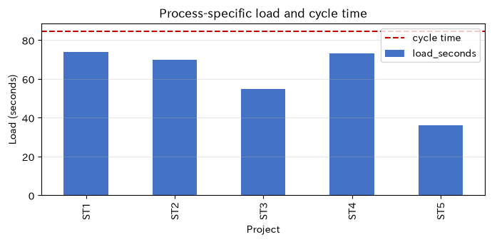
0	ST1	Parts extraction → press-in	74	10.38
1	ST2	conclude → application	70	14.38
2	ST3	adjustment	55	29.38
3	ST4	Power-On Inspection → Visual inspection	73	11.38
4	ST5	Packaging	36	48.38

Cycle time: 84.4 seconds per unit
Train Formation Efficiency: 73.0%

Reading the results

Since the bars of each process fall below the red cycle time line, daily demand can be processed within standard time. However, there are differences in margin between processes, and when the maximum load stops, the load spreads throughout the entire line. Formation efficiency is not a conclusion for capital investment, but a benchmark for re-evaluation through actual measurements including walking, supply, and quality checks.

No.042: Job Shop — Sending Jobs with Different Process Paths

Meaning in Practice

At the Job Shop, the process path differs for each variety. In small-lot, multi-variety production such as prototypes, molds, and spare parts, the coordination that resolves equipment competition and flows each job determines delivery times.

Approach to Analysis and Modeling

The start time for each task is the maximum value of “completion of the previous job task” and “the time when the target equipment becomes available.”

$s_{j,k}=\max(c_{j,k-1},\ a_{m(j,k)})$

Here, dispatching is performed in a fixed job priority order to assign the earliest start time.

Check with Python

routes = {
    "J1": [("cutting", 55), ("grinding", 35), ("inspection", 20)],
    "J2": [("grinding", 45), ("cutting", 30), ("inspection", 18)],
    "J3": [("cutting", 40), ("inspection", 22), ("grinding", 30)],
    "J4": [("inspection", 15), ("cutting", 48), ("grinding", 25)],
}
machine_ready = {m: 0 for m in ["cutting", "grinding", "inspection"]}
job_ready = {j: 0 for j in routes}
schedule = []
for op_no in range(3):
    for job in routes:
        machine, duration = routes[job][op_no]
        start = max(job_ready[job], machine_ready[machine])
        end = start + duration
        schedule.append([job, op_no + 1, machine, start, end, duration])
        job_ready[job] = end
        machine_ready[machine] = end

jobshop = pd.DataFrame(schedule, columns=["jobs", "Smooth engineering", "equipment", "start", "end", "hours"])
display(jobshop.sort_values(["start", "equipment"]))
print(f"All job completion times (makespan）: {jobshop['end'].max()}minutes")

fig, ax = plt.subplots(figsize=(9, 4))
machines = ["cutting", "grinding", "inspection"]
colors = dict(zip(routes, ["#4472C4", "#ED7D31", "#70AD47", "#A5A5A5"]))
for row in jobshop.itertuples():
    y = machines.index(row.equipment)
    ax.barh(y, row.hours, left=row.start, color=colors[row.jobs], edgecolor="white")
    ax.text((row.start + row.end) / 2, y, row.jobs, ha="center", va="center", color="white")
ax.set_yticks(range(len(machines)), machines)
ax.set_title("Gantt Chart by Equipment in Job Shops")
ax.set_xlabel("Time (minutes)")
ax.set_ylabel("equipment")
ax.grid(axis="x", alpha=0.3)
plt.tight_layout()
plt.show()

	jobs	Smooth engineering	equipment	start	end	hours
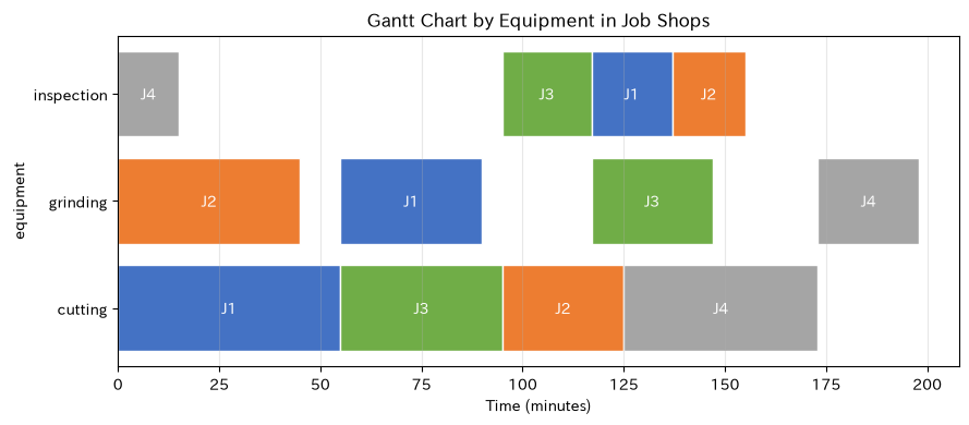
0	J1	1	cutting	0	55	55
3	J4	1	inspection	0	15	15
1	J2	1	grinding	0	45	45
2	J3	1	cutting	55	95	40
4	J1	2	grinding	55	90	35
5	J2	2	cutting	95	125	30
6	J3	2	inspection	95	117	22
8	J1	3	inspection	117	137	20
10	J3	3	grinding	117	147	30
7	J4	2	cutting	125	173	48
9	J2	3	inspection	137	155	18
11	J4	3	grinding	173	198	25

Makespan time for all jobs: 198 minutes

Reading the results

In the blank Gantt chart, waiting for the upstream process and waiting for equipment are mixed. Instead of treating all blanks as “wasteful equipment,” distinguish which constraints caused them. Since changing priority order can affect makespan and job-specific delivery times, you should recalculate the overall impact when cutting in urgent items.

No.043: Flow Shop — Selecting the Order in Which Products Go Through Common Processes

Meaning in Practice

In flow shops where all products pass through equipment in the same order, even the order of entry can affect the time of congestion and end. It can be used to determine the sequence of processes with common paths such as painting, heat treatment, and packaging.

Approach to Analysis and Modeling

For permutation $\pi$, the completion time of job $i$ and process $k$ is

$C_{i,k}=\max(C_{i-1,k}, C_{i,k-1})+p_{\pi_i,k}$

That’s right. If you have 5 jobs, there are $5!=120$ options, so list them all and check the minimum order in makespan.

Check with Python

flow_times = pd.DataFrame(
    [[42, 35, 24], [30, 46, 20], [38, 28, 32], [25, 40, 27], [45, 22, 30]],
    index=["F1", "F2", "F3", "F4", "F5"], columns=["cutting", "grinding", "inspection"]
)

def flowshop_completion(sequence, times=flow_times):
    completion = np.zeros((len(sequence), len(times.columns)), dtype=int)
    for i, job in enumerate(sequence):
        for k, machine in enumerate(times.columns):
            prev_job = completion[i - 1, k] if i > 0 else 0
            prev_machine = completion[i, k - 1] if k > 0 else 0
            completion[i, k] = max(prev_job, prev_machine) + times.loc[job, machine]
    return completion

results = []
for seq in itertools.permutations(flow_times.index):
    c = flowshop_completion(seq)
    results.append((" → ".join(seq), int(c[-1, -1])))
flow_result = pd.DataFrame(results, columns=["Entry order", "makespan_points"]).sort_values("makespan_points")
display(flow_result.head(10))
best_seq = flow_result.iloc[0, 0].split(" → ")
baseline = flowshop_completion(list(flow_times.index))[-1, -1]
best = flow_result.iloc[0, 1]
print(f"Original order: {baseline}minutes / best order: {best}minutes / Abbreviation: {baseline-best}minutes")

ax = flow_result["makespan_points"].plot.hist(bins=12, color="#70AD47", edgecolor="white", figsize=(7, 3.5))
ax.axvline(best, color="#C00000", linestyle="--", label=f"best {best}minutes")
ax.set_title("Entry order120streetmakespandistribution")
ax.set_xlabel("makespan(minutes)")
ax.set_ylabel("permutation number")
ax.grid(axis="y", alpha=0.3)
ax.legend()
plt.tight_layout()
plt.show()

	Entry order	makespan_minutes
80	F4 → F2 → F3 → F1 → F5	232
86	F4 → F3 → F2 → F1 → F5	232
38	F2 → F4 → F3 → F1 → F5	233
74	F4 → F1 → F3 → F2 → F5	233
32	F2 → F3 → F4 → F1 → F5	233
78	F4 → F2 → F1 → F3 → F5	236
24	F2 → F1 → F3 → F4 → F5	236
72	F4 → F1 → F2 → F3 → F5	238
84	F4 → F3 → F1 → F2 → F5	238
57	F3 → F2 → F4 → F5 → F1	239

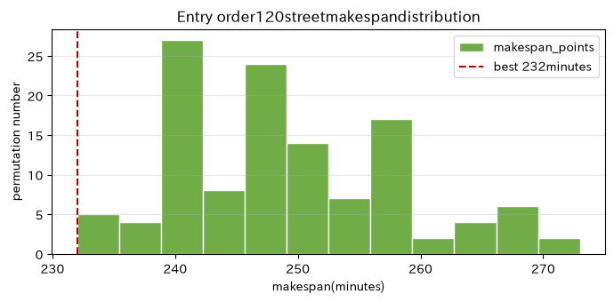
Original order: 248 minutes / Best order: 232 minutes / Shortened: 16 minutes

Reading the results

It is clear that simply changing the order of deployment without increasing equipment capacity can shorten the end time. On the other hand, the shortest makespan order does not always guarantee individual delivery deadlines. When applied on-site, setup time, material arrival, and delivery priority are also added to the objective function and constraint.

No.044: Scheduling — Comparing EDD and SPT by Delivery KPIs

Meaning in Practice

Even with a single facility, the on-time delivery rate varies depending on which tasks are processed first. By comparing the representative EDD (order of fastest delivery time) and SPT (order of shortest processing time), you can clearly state the aim of the on-site rules.

Approach to Analysis and Modeling

The delay in job $j$ is $T_j=\max(0,C_j-d_j)$. EDD tends to reduce maximum latency, while SPT tends to reduce average dwell time. Break down evaluation metrics into total delays, number of delays, and average completion time.

Check with Python

def evaluate_rule(df, sort_col):
    x = df.sort_values(sort_col).copy()
    x["completed_minutes"] = x["processing_time_minutes"].cumsum()
    x["late_minutes"] = (x["completed_minutes"] - x["delivery_time_minutes"]).clip(lower=0)
    return x

edd = evaluate_rule(orders, "delivery_time_minutes")
spt = evaluate_rule(orders, "processing_time_minutes")
comparison = pd.DataFrame({
    "Rules": ["EDD(Delivery date, order of delivery)", "SPT(Shortest duration order)"],
    "total_delay_by_minutes": [edd["late_minutes"].sum(), spt["late_minutes"].sum()],
    "Number of delays": [(edd["late_minutes"] > 0).sum(), (spt["late_minutes"] > 0).sum()],
    "average_completed_minutes": [edd["completed_minutes"].mean(), spt["completed_minutes"].mean()],
})
display(comparison)
print("EDDOrder:", " → ".join(edd["jobs"]))
print("SPTOrder:", " → ".join(spt["jobs"]))

ax = comparison.set_index("Rules")[["total_delay_by_minutes", "average_completed_minutes"]].plot.bar(
    color=["#C00000", "#4472C4"], figsize=(7, 3.8), rot=0
)
ax.set_title("By Dispatching RulesKPI")
ax.set_xlabel("Rules")
ax.set_ylabel("Time (minutes)")
ax.grid(axis="y", alpha=0.3)
plt.tight_layout()
plt.show()

	Rules	total_delay_by_minutes	Number of delays	average_completed_minutes
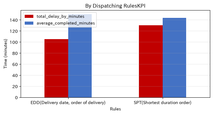
0	EDD(Delivery date, order of delivery)	105	3	150.00
1	SPT(Shortest duration order)	130	1	143.33

EDD order: J4 → J2 → J6 → J1 → J3 → J5
SPT order: J4 → J2 → J6 → J3 → J5 → J1

Reading the results

Which is better depends on the KPI. If you prioritize meeting deadlines, prioritize delay indicators; if you prioritize reducing work in progress, prioritize average completion time. It serves as material for numerically comparing implicit rules like “traditional delivery date” and using different rules for each order category.

No.045: Formulating constraints — Verifying the feasibility of production plans

Meaning in Practice

If sales plans are directly translated into manufacturing instructions, certain equipment may exceed capacity. By using constraint methods, you can explain the causes of planned failure and the required overtime or outsourcing time by process.

Approach to Analysis and Modeling

If we $x_p$ the quantity of product $p$, $a_{mp}$ the standard time of process $m$, and $b_m$ available time, the capacity constraint is

$\sum_p a_{mp}x_p \le b_m \quad (\forall m)$

That’s right. Additionally, $x_p\ge0$ set integer conditions, demand limits, and material constraints if necessary. Here, we diagnose the constraints and margin of the proposal to produce according to demand.

Check with Python

machines = ["cutting", "grinding", "inspection"]
available = pd.Series({"cutting": 450, "grinding": 450, "inspection": 420}, name="available_minutes")
time_cols = [f"{m}_minutes" for m in machines]
load = pd.Series(
    products[time_cols].to_numpy().T @ products["daily demand"].to_numpy(),
    index=machines, name="required_load_minutes"
)
constraints = pd.concat([load, available], axis=1)
constraints["yu_li_fen"] = constraints["available_minutes"] - constraints["required_load_minutes"]
constraints["load factor"] = constraints["required_load_minutes"] / constraints["available_minutes"]
constraints["executable"] = constraints["yu_li_fen"] >= 0
display(constraints)
print("Feasibility of the entire plan:", "executable" if constraints["executable"].all() else "Violation of capability constraints")

ax = constraints[["required_load_minutes", "available_minutes"]].plot.bar(
    color=["#ED7D31", "#A5A5A5"], figsize=(7, 3.5), rot=0
)
ax.set_title("Required load and available time by process")
ax.set_xlabel("Project")
ax.set_ylabel("Time (minutes)/Day)")
ax.grid(axis="y", alpha=0.3)
plt.tight_layout()
plt.show()

	required_load_minutes	available_minutes	surplus_strength_minutes	load factor	executable
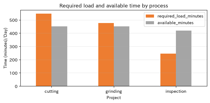
cutting	547.20	450	-97.20	1.22	False
grinding	475.20	450	-25.20	1.06	False
inspection	244.80	420	175.20	0.58	True

Overall Feasibility of the Plan: Violating Capacity Constraints

Reading the results

Processes that violate restrictions are the reason why daily plans cannot be executed as is. Even if the load rate is below 100%, if the fluctuating absorption margin is small, it is dangerous in practice. First, separate standard hours from stoppages, and compare costs and delivery times to secure extra capacity through overtime, outsourcing, or quantity adjustment.

No.046: Simulation Optimization — Selecting Personnel Proposals Under Variability

Meaning in Practice

If you decide personnel based solely on average standard time, daily variability can lead to unmet plans. Generate many “virtual days” for each proposal and compare the probability of completion with the cost.

Approach to Analysis and Modeling

Expected loss for each $x$ plan

$J(x)=C_{\mathrm{labor}}(x)+C_{\mathrm{short}}\,\mathbb{E}[\max(0,D-Q(x,\omega))]$

Let’s say so. $\omega$ is the random number of processing times and stops, and $Q$ is the daily output. Here, we compare the 2–5 person proposals using common random numbers and select the option with the lowest cost.

Check with Python

sim_rng = np.random.default_rng(SEED)
n_sim = 5000
demand = 320
base_cycle = sim_rng.lognormal(mean=np.log(70), sigma=0.10, size=n_sim)
downtime = np.clip(sim_rng.normal(35, 18, size=n_sim), 0, 120)

sim_rows = []
for workers in range(2, 6):
    # Assuming the effectiveness of concurrent work diminishes
    effective_lines = 1 + 0.72 * (workers - 2)
    available_seconds = (450 - downtime) * 60
    output = np.floor(available_seconds / base_cycle * effective_lines)
    shortage = np.maximum(0, demand - output)
    daily_cost = workers * 18000 + shortage.mean() * 2500
    sim_rows.append([workers, output.mean(), np.quantile(output, 0.05), (output >= demand).mean(), daily_cost])

sim_options = pd.DataFrame(sim_rows, columns=["Number of personnel", "Average production quantity", "5%Quile production", "Required Completion Probability", "expected_total_cost_yen"])
display(sim_options)
best_worker = int(sim_options.loc[sim_options["expected_total_cost_yen"].idxmin(), "Number of personnel"])
print(f"Proposals with the Lowest Expected Total Cost: {best_worker}person")

fig, ax1 = plt.subplots(figsize=(7.5, 3.8))
ax1.plot(sim_options["Number of personnel"], sim_options["Required Completion Probability"], marker="o", color="#4472C4")
ax1.set_xlabel("Number of personnel")
ax1.set_ylabel("Required Completion Probability", color="#4472C4")
ax1.set_ylim(0, 1.05)
ax2 = ax1.twinx()
ax2.plot(sim_options["Number of personnel"], sim_options["expected_total_cost_yen"], marker="s", color="#C00000")
ax2.set_ylabel("Expected total cost (yen)/Day)", color="#C00000")
ax1.set_title("Probability of meeting demand and expected total cost of personnel proposals")
ax1.grid(alpha=0.3)
plt.tight_layout()
plt.show()

	Number of personnel	Average production quantity	5%Quile production	Required Completion Probability	expected_total_cost_jpy
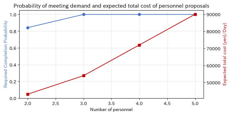
0	2	357.49	298.00	0.84	43,167.00
1	3	615.25	513.00	1.00	54,000.00
2	4	873.01	728.00	1.00	72,000.00
3	5	1,130.76	943.00	1.00	90,000.00

Proposal with the lowest expected total cost: 2 people

Reading the results

The more people you have, the higher the chances of success, but so do labor costs. Since the minimum expected cost proposal depends on the assumed shortage unit price, it is practical to analyze sensitivity rather than fixing the unit price at a single point. Also, by listing not only average production volume but also the 5% percentile points, you can understand supply capacity on bad days.

No.047: Bottleneck Analysis — Identifying Processes That Constrain Overall Throughput

Meaning in Practice

Even if all processes are improved evenly, the total shipment volume will not increase at the same ratio. The Constraints Theory (TOC) approach identifies the most pressing processes and prioritizes operations that do not stop them.

Approach to Analysis and Modeling

Compare process load factor $u_m=L_m/B_m$, and consider the largest process as a provisional bottleneck. However, in practice, since movement occurs due to blocking, material waiting, and breakdowns, both load rate and queues are used together.

Check with Python

bottleneck = constraints.copy()
bottleneck["residual capacity rate"] = 1 - bottleneck["load factor"]
bn_name = bottleneck["load factor"].idxmax()
display(bottleneck.sort_values("load factor", ascending=False))
print(f"Potential Bottleneck in Planning: {bn_name}")

colors = ["#C00000" if x == bn_name else "#4472C4" for x in bottleneck.index]
ax = (bottleneck["load factor"] * 100).plot.bar(color=colors, figsize=(7, 3.5), rot=0)
ax.axhline(100, color="black", linestyle="--", label="Ability Ceiling")
ax.set_title("Bottleneck candidates based on process load rates")
ax.set_xlabel("Project")
ax.set_ylabel("Load Factor (%）")
ax.grid(axis="y", alpha=0.3)
ax.legend()
plt.tight_layout()
plt.show()

	required_load_minutes	available_minutes	surplus_strength_minutes	load factor	executable	residual capacity rate
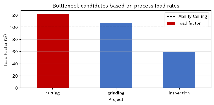
cutting	547.20	450	-97.20	1.22	False	-0.22
grinding	475.20	450	-25.20	1.06	False	-0.06
inspection	244.80	420	175.20	0.58	True	0.42

Potential Bottleneck in Planning: Cutting

Reading the results

The red process is the first candidate for improvement. In the short term, downtime will be reduced through break rotations, advance material supply, and out-of-setup setup; in the medium term, processing conditions, jigs, outsourcing, and expansion will be considered. Since maximizing the utilization rate of all equipment increases by running non-bottleneck areas at high capacity, we avoid maximizing the utilization rate of all equipment.

No.048: Tact Time — Determining Production Pace and Number of Staff to Meet Demand

Meaning in Practice

Takt time refers to the production pace required by customer demand. By comparing with standard times, you can make the required number of parallel lines and participants, as well as support decisions by time of day, a common language.

Approach to Analysis and Modeling

For $T$ net operating hours and $D$ demand,

$\text{Takt}=\frac{T}{D},\qquad n_{\min}=\left\lceil\frac{\text{Total working time}}{\text{Takt}}\right\rceil$

That’s right. Tact is not actual cycle time. The former is the demand baseline, while the latter is process capability.

Check with Python

demands = np.array([260, 300, 320, 360, 400])
net_available_sec = 7.5 * 3600
work_content_sec = assembly_tasks["standard_time_seconds"].sum()
takt_table = pd.DataFrame({"daily demand": demands})
takt_table["tact_seconds"] = net_available_sec / takt_table["daily demand"]
takt_table["theoretical minimum number of people"] = np.ceil(work_content_sec / takt_table["tact_seconds"]).astype(int)
display(takt_table)

fig, ax1 = plt.subplots(figsize=(7, 3.8))
ax1.plot(takt_table["daily demand"], takt_table["tact_seconds"], marker="o", color="#4472C4")
ax1.set_xlabel("Daily Needs (pcs)")
ax1.set_ylabel("Tact time (seconds)/Individual)")
ax2 = ax1.twinx()
ax2.step(takt_table["daily demand"], takt_table["theoretical minimum number of people"], where="mid", color="#ED7D31")
ax2.set_ylabel("theoretical minimum number of people")
ax1.set_title("Takt time and required number of people in response to demand changes")
ax1.grid(alpha=0.3)
plt.tight_layout()
plt.show()

	daily demand	tact_seconds	theoretical minimum number of people
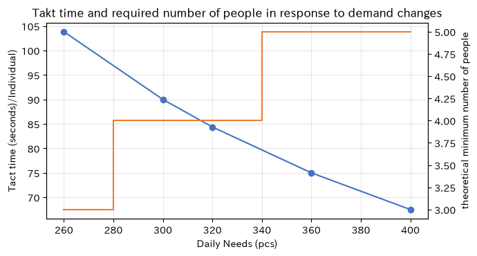
0	260	103.85	3
1	300	90.00	4
2	320	84.38	4
3	360	75.00	5
4	400	67.50	5

Reading the results

As demand increases, the tact shortens, and the number of people needed gradually increases at a certain boundary. The theoretical minimum number of players is the lower limit that does not include team loss, fatigue margin, or cheering skills. S&OP shows boundaries for each demand scenario and serves as a leading indicator for hiring, multi-skilled workers, and overtime.

No.049: Production Capacity Analysis — Measuring the Probability of Demand Fulfillment, Including OEE Fluctuations

Meaning in Practice

Even if the nominal capacity exceeds demand, stopping, speed drops, and defects reduce effective capability. When ability is treated as a probability distribution, you can move the judgment from “on average” to “what percentage of probability is enough.”

Approach to Analysis and Modeling

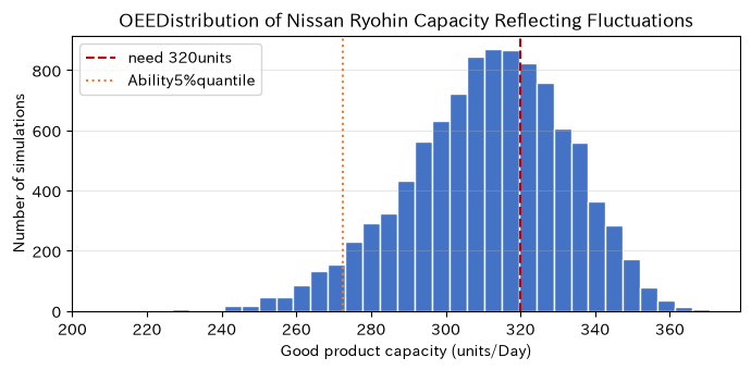
OEE is the product $A\times P\times Q$ of $A$ operating rate, $P$ performance, and $Q$ quality rate, and Nissan capacity

$K=K_{\mathrm{ideal}}\times A\times P\times Q$

Calculate it as follows. Each element is evaluated as a random number between 0 and 1 in Monte Carlo. For strongly correlated real data, the same pair is resampled from the same day rather than an independent random number.

Check with Python

cap_rng = np.random.default_rng(SEED)
n = 10000
availability = cap_rng.beta(45, 5, n)
performance = cap_rng.beta(38, 4, n)
quality = cap_rng.beta(98, 2, n)
ideal_capacity = 390
oee = availability * performance * quality
capacity = ideal_capacity * oee
demand_target = 320

capacity_kpi = pd.Series({
    "averageOEE": oee.mean(),
    "Average Good Yield Capacity": capacity.mean(),
    "ability5%quantile": np.quantile(capacity, 0.05),
    "Required Completion Probability": (capacity >= demand_target).mean(),
})
display(capacity_kpi.to_frame("value"))

fig, ax = plt.subplots(figsize=(7, 3.5))
ax.hist(capacity, bins=35, color="#4472C4", edgecolor="white")
ax.axvline(demand_target, color="#C00000", linestyle="--", label=f"need {demand_target}units")
ax.axvline(np.quantile(capacity, 0.05), color="#ED7D31", linestyle=":", label="ability5%quantile")
ax.set_title("OEEDistribution of Nissan Ryohin Capacity Reflecting Fluctuations")
ax.set_xlabel("Good product capacity (units/Day)")
ax.set_ylabel("Number of simulations")
ax.grid(axis="y", alpha=0.3)
ax.legend()
plt.tight_layout()
plt.show()

	value
averageOEE	0.80
Average Good Yield Capacity	311.13
ability5%quantile	272.48
Required Completion Probability	0.36

Reading the results

The area to the left of the demand line is the probability of not being reached. Looking at not only average capacity but also the 5% percentile allows you to reflect supply capacity on tight days in inventory policies and delivery time responses. Since OEE multipliers alone can hide the reasons for losses, we individually improve and manage uptime, performance, and quality.

No.050: Digital Twin — Update Status and Compare the Future with On-Site Performance

Meaning in Practice

Digital twins are not just clean 3D displays. This system connects equipment, schedules, standard times, and plans with on-site events, reproduces the current state, and compares the results of measures before they impact reality.

Approach to Analysis and Modeling

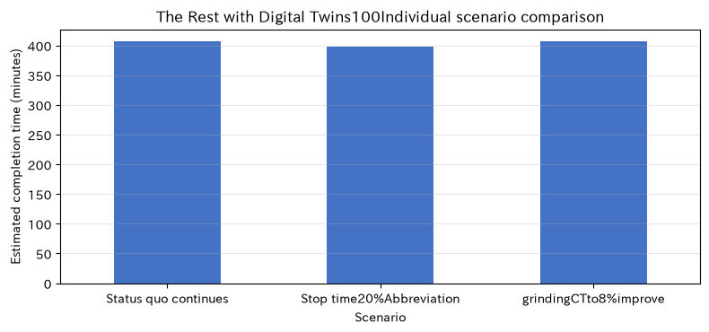
The minimum configuration is: (1) target and KPIs, (2) state data, (3) update rules, (4) forecasting and simulation, (5) decision-making, and (6) performance feedback. This time, we update the cycle times by process based on the most recent completion event and compare the expected completion of the current plan with the shortened shutdown plan.

Exponential smoothing that updates the estimate $\hat\mu_t$ at observation $y_t$ is

$\hat\mu_t=\alpha y_t+(1-\alpha)\hat\mu_{t-1}$

That’s right. Don’t abruptly abandon old standards and reflect recent changes.

Check with Python

twin_rng = np.random.default_rng(SEED)
event_rows = []
standards = {"cutting": 3.5, "grinding": 3.2, "inspection": 1.6}
for machine, standard in standards.items():
    observed = twin_rng.lognormal(np.log(standard), 0.12, 30)
    for i, value in enumerate(observed, 1):
        event_rows.append([f"E-{machine}-{i:02d}", machine, i, value])
events = pd.DataFrame(event_rows, columns=["event_id", "Project", "order of completion", "achievements_ct"])

alpha = 0.25
state_rows = []
for machine, group in events.groupby("Project", sort=False):
    estimate = standards[machine]
    for value in group["achievements_ct"]:
        estimate = alpha * value + (1 - alpha) * estimate
    state_rows.append([machine, standards[machine], estimate])
twin_state = pd.DataFrame(state_rows, columns=["Project", "standard_ct_points", "update_ct_minutes"]).set_index("Project")
twin_state["Deviation rate"] = twin_state["update_ct_minutes"] / twin_state["standard_ct_points"] - 1
display(twin_state)

remaining = 100
scenario = pd.DataFrame({
    "Scenario": ["Status quo continues", "Stop time20%Abbreviation", "grindingCTto8%improve"],
    "expected_stop_minutes": [45, 36, 45],
    "grindingCTcoefficient": [1.0, 1.0, 0.92],
})
base_ct = twin_state["update_ct_minutes"].max()
scenario["estimated_completion_in_minutes"] = scenario["expected_stop_minutes"] + remaining * np.maximum(
    [base_ct, base_ct, twin_state.loc["grinding", "update_ct_minutes"] * 0.92]
, twin_state.drop(index="grinding")["update_ct_minutes"].max())
display(scenario)

ax = scenario.plot.bar(x="Scenario", y="estimated_completion_in_minutes", color="#4472C4", legend=False, figsize=(8, 3.8), rot=0)
ax.set_title("The Rest with Digital Twins100Individual scenario comparison")
ax.set_xlabel("Scenario")
ax.set_ylabel("Estimated completion time (minutes)")
ax.grid(axis="y", alpha=0.3)
plt.tight_layout()
plt.show()

	StandardCT_minutes	UpdateCT_minutes	Deviation rate
Project
cutting	3.50	3.61	0.03
grinding	3.20	3.28	0.03
inspection	1.60	1.62	0.01

	Scenario	expected_stop_minutes	grindingCTcoefficient	estimated_completion_in_minutes
0	Status quo continues	45	1.00	406.42
1	Stop time20%Abbreviation	36	1.00	397.42
2	grindingCTto8%improve	45	0.92	406.42

Reading the results

A discrepancy between the standard and updated values is a signal to review the planning master. The scenario table compares the effects of “Shortened Stop” and “Cycle Improvement” at the same expected completion time. In production, event deviations, time deviations, and equipment status codes are monitored, and discrepancies between model values and actual results are continuously recorded. Even when automating model updates, the final authority for manufacturing instructions and the manual resumption procedure in case of abnormalities are clearly defined.

Practical Implications Seen Through Target Exercise

1. Calculate backward from demand: Tacit and required capabilities are defined in advance, and high utilization of individual equipment is not set as the goal.
2. Order is also an ability.: In job shops and flow shops, there is room for improvement even without adding equipment.
3. Specify constraints: By formulating time, materials, personnel, and contextual relationships, the reasons for plan failure can be shared among relevant departments.
4. From average values to probability: Using demand fulfillment probability and downward quantiles, you can design a safety margin against fluctuations.
5. Focus on bottlenecks: Rather than partial optimization of non-constrained processes, priority is given to protecting and improving processes that restrict shipment.
6. Returning the performance to the model: Digital twins are not created once but operate by updating standards and logic using prediction errors.

What is necessary for practical implementation

1. Decide on Decisions and KPIs First

Instead of “what to visualize,” define “who decides which options, when, and which options.” For daily differentials, the main KPIs are delivery deadlines, work in progress, and overtime; for capital investment, the main KPIs are capacity decline, demand scenarios, and investment recovery.

2. Align the meaning of the master and achievements

We unify definitions of items, process sequence, equipment capacity, calendar, scheduling, and quality and rework. Standard time plate management and the granularity of stop reason codes determine analysis accuracy.

3. Start with a small closed loop

Within one product group and one line, we run ‘Actual Collection→ Status Updates→ Creation of Next-Day Plans→ On-site Inspection→ Result Evaluation.’ After verifying value with spreadsheets and notebooks, we gradually increase integration with MES, ERP, and equipment data.

4. Embed constraints and separation of responsibilities into operations

Reflect freezing periods, emergency items, maintenance schedules, and quality isolations in the model, and leave the reasons for adopting or rejecting automated proposals. Alternative procedures for model stoppages, approval permissions, and audit logs are also part of the design.

Conclusion

No.041 to No.050 covered work allocation, process conflicts, input order, delivery rules, finite capacity, variable evaluation, constrained processes, demand pace, probabilistic capability, and performance feedback.

The quality of production planning is not determined solely by optimization algorithms. Only when the correct process master, realistic constraints, multiple KPIs, handling variation, and updunable operations on site are in place can planning be used for decision-making. It is reliable to start by creating baseline values for small subjects and expanding accuracy and applicability by measuring the difference between predictions and actual results.

Consultations for Corporations

At Surikoubo, we offer consultations for everything from production planning and scheduling, simulation, mathematical optimization, and digital twin conceptualization to implementation and in-house production support in manufacturing.

• Design of production planning models reflecting process, equipment, and personnel constraints
• Bottleneck analysis, capability evaluation, and establishment of inventory and delivery KPIs
• Simulation and Investment Effect Verification Using On-site Data
• Building a decision-making platform that connects ERP, MES, and equipment data
• Corporate training covering Python, statistics, and optimization

📩 Contact Us: surikobo.co.jp/contact
Please feel free to consult us first.