Shifting Existing Customers from ‘Sales’ to ‘Relationships’: 10 Key Customer Strategies for Industrial Parts Manufacturers

This article uses the two-year order history and promotional experiments of the fictional industrial parts manufacturer ‘Suiri Seiki’ as a subject to treat Customer prioritization, understanding retention rates, verifying the effectiveness of initiatives, forecasting future value, and cross-selling as a single decision-making process. Through No.051 to No.060, you will see how to move from sales management that merely looks at aggregates to customer strategies where each customer can choose “what to do next.”

[!NOTE] This material is a notebook previously used by Surikoubo (or personally by the representative, Kazuyama), and has been reconstructed, edited, and published with the company’s permission.
All data listed is fictional and has no relation whatsoever to real companies, factories, or figures.

Introduction: Practical Challenges in Manufacturing Covered in This Article

Marketing in manufacturing is not just about advertising. It is also important to maintain long-term relationships with agents, equipment manufacturers, and maintenance departments, and to propose repair items and related materials at the appropriate time. However, if you approach ‘visiting because sales are high,’ ‘noticing loss after losing orders,’ or ‘counting only campaign responders as successful,’ you cannot effectively allocate sales effort and discount resources.

Here, order histories are reinterpreted by customer, acquisition timing, and order units, and using descriptive statistics, probabilistic models, machine learning, and randomized controlled trials to create shareable decision-making materials for sales, marketing, and production planning.

Common situations on site

• Core systems have order history, but customer priorities depend on the experience of the person in charge
• While tracking new customer numbers, they do not look at retention rates by month of acquisition.
• Post-exhibition emails and technical consultation sessions are distributed simultaneously to all customers
• Unable to distinguish between customers whose orders have stopped and those whose purchase cycles are only long.
• You know sales by product, but don’t know what to buy simultaneously or what product to propose next.
• Even if the purchase rate after the policy is high, it cannot be ruled out that the original customers were the buyers.

Why is this issue so difficult to judge?

Corporate customers have uneven purchase intervals, with varying sizes and equipment renewal cycles for each customer. Therefore, the average number of purchases alone can be a mix of “dormancy” and “normal long intervals.” Also, when selecting the target of a campaign and measuring its effectiveness using the same data, it is easy to mistakenly interpret the effect of selecting customers with high purchase intent as the effectiveness of the campaign.

What is needed is to separate the units of analysis according to the purpose. At the customer level, use RFM, churn, and CLV; on the acquisition month, use cohort; on the order basis, use basket; and at the initiative level, use A/B testing and Uplift. Each metric is not a “higher is better” evaluation, but is used to determine To which customers, at which touchpoints, and to what extent to spend.

Overview of Exercise covered this time

No.	Theme	Key Decisions
051	RFM Analysis	Priority for sales follow-up
052	Cohort Analysis	Improvement of acquisition strategies and onboarding
053	A/B Testing	Will we roll out initiatives company-wide?
054	Customer churn analysis	Who should we respond to dormant signs?
055	Pareto/NBD	Capturing the difference in purchase frequency between customers using probabilistic means
056	BG/NBD	Estimating survival probabilities including purchase stops
057	CLV	Set investment limits for each client
058	Market Basket Analysis	Discover cross-cell combinations
059	Recommendation System	Create the next product candidates by customer
060	Uplift Modeling	Choose customers whose actions change through your actions

Preparing the Python environment

numpy, pandas, scipy, scikit-learn, and matplotlib are used. The random number generator is initialized with a fixed seed so that no matter how many times it runs, the same fictitious data and results are obtained.

import itertools
import warnings

import japanize_matplotlib
import matplotlib.pyplot as plt
import numpy as np
import pandas as pd
from scipy import stats
from sklearn.linear_model import LogisticRegression
from sklearn.metrics import RocCurveDisplay, roc_auc_score
from sklearn.metrics.pairwise import cosine_similarity
from sklearn.model_selection import train_test_split

warnings.filterwarnings("ignore")
pd.set_option("display.max_columns", 20)
pd.set_option("display.float_format", lambda x: f"{x:,.3f}")

SEED = 202507
rng = np.random.default_rng(SEED)
ANALYSIS_END = pd.Timestamp("2025-12-31")
print("Analysis Reference Date:", ANALYSIS_END.date(), " / seed:", SEED)

Analysis reference date: 2025-12-31 / seed: 202507

Creation of Fictional Data

Generate customer masters for 600 companies, order headers for January 2024 to December 2025, and order slips. Purchase frequency, unit price, and dormancy vary by customer segment, and certain product categories are often selected simultaneously within an order. This is fictitious data intended to explain the analysis procedure and is not a benchmark to guarantee model performance.

n_customers = 600
segments = np.array(["Equipment Manufacturers", "agency", "Conservation department", "Research and Development"])
segment = rng.choice(segments, n_customers, p=[0.30, 0.25, 0.30, 0.15])
cohort_month = rng.integers(0, 12, n_customers)
customers = pd.DataFrame({
    "customer_id": [f"C{i:04d}" for i in range(1, n_customers + 1)],
    "segment": segment,
    "cohort": pd.Timestamp("2024-01-01") + pd.to_timedelta(cohort_month * 30.44, unit="D"),
})
customers["cohort"] = customers["cohort"].dt.to_period("M").dt.to_timestamp()

rate_map = {"Equipment Manufacturers": 0.75, "agency": 1.05, "Conservation department": 0.52, "Research and Development": 0.32}
amount_map = {"Equipment Manufacturers": 320_000, "agency": 210_000, "Conservation department": 145_000, "Research and Development": 110_000}
product_names = np.array(["bearing", "Seal", "lubricant", "Sensors", "control component", "Maintenance Kit"])
base_product_p = np.array([0.23, 0.18, 0.14, 0.17, 0.14, 0.14])

orders_data, lines_data = [], []
order_no = 1
for row in customers.itertuples(index=False):
    latent = rng.gamma(shape=1.8, scale=0.7)
    dropout_month = rng.choice(np.arange(8, 30), p=np.repeat(1 / 22, 22))
    for month in pd.date_range(row.cohort, ANALYSIS_END, freq="MS"):
        age = (month.year - row.cohort.year) * 12 + month.month - row.cohort.month
        if age >= dropout_month:
            break
        n_orders = rng.poisson(rate_map[row.segment] * latent)
        for _ in range(n_orders):
            order_id = f"O{order_no:06d}"
            date = month + pd.Timedelta(days=int(rng.integers(0, 27)))
            amount = max(25_000, rng.lognormal(np.log(amount_map[row.segment]), 0.45))
            orders_data.append((order_id, row.customer_id, date, amount, amount * rng.uniform(0.24, 0.38)))
            n_items = int(rng.integers(1, 4))
            items = list(rng.choice(product_names, size=n_items, replace=False, p=base_product_p))
            if "bearing" in items and "lubricant" not in items and rng.random() < 0.42:
                items.append("lubricant")
            if "Sensors" in items and "control component" not in items and rng.random() < 0.38:
                items.append("control component")
            weights = rng.dirichlet(np.ones(len(items)))
            for item, weight in zip(items, weights):
                lines_data.append((order_id, row.customer_id, date, item, amount * weight))
            order_no += 1

orders = pd.DataFrame(orders_data, columns=["order_id", "customer_id", "order_date", "sales", "gross_profit"])
order_lines = pd.DataFrame(lines_data, columns=["order_id", "customer_id", "order_date", "product", "line_sales"])
customers = customers.merge(orders.groupby("customer_id")["order_date"].min().rename("first_order"), on="customer_id", how="left")

print(f"number_of_customers: {len(customers):,}society / Order quantity: {len(orders):,}records / detailed quantity: {len(order_lines):,}rows")
display(orders.head())
display(order_lines.head())

Number of customers: 600 / Number of orders: 8,440 / Number of details: 18,942 lines

	order_id	customer_id	order_date	sales	gross_profit
0	O000001	C0001	2024-11-20	186,215.307	48,156.255
1	O000002	C0001	2024-11-22	271,079.760	100,379.747
2	O000003	C0001	2024-12-19	397,117.855	104,551.397
3	O000004	C0001	2025-01-24	288,861.018	88,361.531
4	O000005	C0001	2025-01-12	140,191.611	41,564.577

	order_id	customer_id	order_date	product	line_sales
0	O000001	C0001	2024-11-20	Sensors	186,215.307
1	O000002	C0001	2024-11-22	Seal	271,079.760
2	O000003	C0001	2024-12-19	lubricant	72,430.084
3	O000003	C0001	2024-12-19	bearing	224,157.931
4	O000003	C0001	2024-12-19	Seal	100,529.840

No.051: RFM Analysis — Visualizing Sales Follow-up Priorities

Meaning in Practice

RFMs organize customers by the number of days from last purchase (Recency), Number of Purchases (Frequency), and Purchase Amount (Monetary). In manufacturing, practical applications include not only identifying key customers but also early identifying large customers whose orders have recently stopped.

Approach to Analysis and Modeling

If the base date for customer (i) is (t_0), it is (R_i=t_0-\max(t_{ij})), (F_i=\sum_j 1), and (M_i=\sum_j y_{ij}). Convert each value into a quintile score. Note that the smaller the Recency, the higher the score. Since scores are based on relative evaluation, if the business unit or distribution channel differs, the population is divided.

Check with Python

rfm = orders.groupby("customer_id").agg(
    recency=("order_date", lambda s: (ANALYSIS_END - s.max()).days),
    frequency=("order_id", "nunique"),
    monetary=("sales", "sum"),
).reset_index()
rfm["R"] = pd.qcut(rfm["recency"].rank(method="first"), 5, labels=[5, 4, 3, 2, 1]).astype(int)
rfm["F"] = pd.qcut(rfm["frequency"].rank(method="first"), 5, labels=[1, 2, 3, 4, 5]).astype(int)
rfm["M"] = pd.qcut(rfm["monetary"].rank(method="first"), 5, labels=[1, 2, 3, 4, 5]).astype(int)
rfm["rfm_score"] = rfm[["R", "F", "M"]].sum(axis=1)
rfm["action"] = np.select(
    [(rfm["R"] >= 4) & (rfm["F"] >= 4), (rfm["R"] <= 2) & (rfm["M"] >= 4)],
    ["Relationship Maintenance and Additional Proposals", "Priority confirmation for dormancy prevention"], default="Standard Follow")

display(rfm.sort_values("rfm_score", ascending=False).head(8))
summary_rfm = rfm.groupby("action").agg(number_of_customers=("customer_id", "size"), average_last_purchase_days=("recency", "mean"), total_sales=("monetary", "sum"))
display(summary_rfm)

fig, ax = plt.subplots(figsize=(8, 5))
for label, group in rfm.groupby("action"):
    ax.scatter(group["recency"], group["monetary"] / 1e6, s=18 + group["frequency"] * 1.5, alpha=0.55, label=label)
ax.set_title("RFMCustomer Portfolio by")
ax.set_xlabel("Number of days since last purchase (the shorter, the more recent)")
ax.set_ylabel("Cumulative Sales (million yen)")
ax.grid(True, alpha=0.3)
ax.legend()
plt.tight_layout()
plt.show()

	customer_id	recency	frequency	monetary	R	F	M	rfm_score	action
419	C0433	13	33	6,467,242.980	5	5	5	15	Relationship Maintenance and Additional Proposals
160	C0164	9	27	5,765,718.503	5	5	5	15	Relationship Maintenance and Additional Proposals
32	C0034	10	54	13,266,440.442	5	5	5	15	Relationship Maintenance and Additional Proposals
480	C0496	8	92	20,833,182.841	5	5	5	15	Relationship Maintenance and Additional Proposals
229	C0237	22	31	12,553,838.924	5	5	5	15	Relationship Maintenance and Additional Proposals
490	C0506	8	34	11,936,063.720	5	5	5	15	Relationship Maintenance and Additional Proposals
207	C0215	6	28	6,283,201.950	5	5	5	15	Relationship Maintenance and Additional Proposals
560	C0581	6	44	10,243,495.304	5	5	5	15	Relationship Maintenance and Additional Proposals

	number_of_customers	average_last_purchase_days	total_sales
action
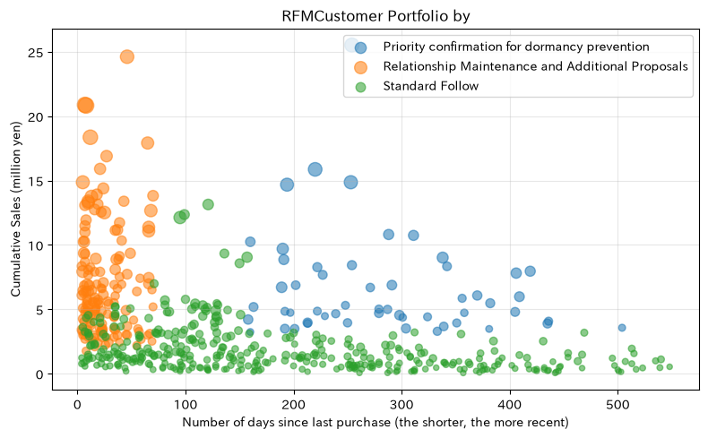
Priority confirmation for dormancy prevention	54	282.037	356,696,374.013
Standard Follow	376	191.694	676,451,584.568
Relationship Maintenance and Additional Proposals	150	24.980	1,052,182,288.200

Reading the results

In the upper right corner, you’ll see customers who have had significant past sales but haven’t bought recently. This group should prioritize confirming reasons for order suspensions, such as equipment stoppages, changes in responsibility, or competitive switches, rather than uniform discounts. On the other hand, customers who are frequently on the left side are subject to relationship maintenance measures such as stockout prevention and annual contracts. Since RFM alone cannot determine causality or future value, it is combined with subsequent analyses.

No.052: Cohort Analysis — Comparing Post-Acquisition Retention on the Same Time Axis

Meaning in Practice

Even if monthly sales are growing, the increase in new acquisition may be masking the loss of existing customers. By reviewing the retention rate by the first order month, you can evaluate the “quality of long-term transactions” of acquisition strategies such as exhibitions, agent introductions, and web inquiries.

Approach to Analysis and Modeling

Let customer (i) have the first purchase month as (c_i), the purchase month as (t), and calculate the elapsed month (a = t - c_i). The retention rate for cohort (c) is (Retention_{c,a} = N_{c,a} / N_{c,0}). For cohorts close to the end of the observation period, the right side is not observed, so it is not filled with zero and treated as a deficiency.

Check with Python

cohort_base = orders.assign(order_month=orders["order_date"].dt.to_period("M").dt.to_timestamp())
first_month = cohort_base.groupby("customer_id")["order_month"].min().rename("cohort")
cohort_base = cohort_base.join(first_month, on="customer_id")
cohort_base["age"] = ((cohort_base["order_month"].dt.year - cohort_base["cohort"].dt.year) * 12 + cohort_base["order_month"].dt.month - cohort_base["cohort"].dt.month)
cohort_counts = cohort_base.groupby(["cohort", "age"])["customer_id"].nunique().unstack()
retention = cohort_counts.div(cohort_counts[0], axis=0)
display((retention.iloc[:, :13] * 100).round(1))

fig, ax = plt.subplots(figsize=(9, 5))
for cohort, row in retention.iloc[:, :13].iterrows():
    ax.plot(row.index, row.values * 100, marker="o", alpha=0.55, label=cohort.strftime("%Y-%m"))
ax.set_title("Customer retention rate by first order month")
ax.set_xlabel("Elapsed months since initial order received")
ax.set_ylabel("Purchase rate for the month (%）")
ax.grid(True, alpha=0.3)
ax.legend(ncol=3, fontsize=8)
plt.tight_layout()
plt.show()

age	0	1	2	3	4	5	6	7	8	9	10	11	12
cohort
2024-01-01	100.000	72.500	68.600	66.700	68.600	74.500	62.700	68.600	68.600	56.900	64.700	51.000	51.000
2024-02-01	100.000	50.000	55.600	44.400	50.000	66.700	72.200	38.900	27.800	38.900	33.300	38.900	38.900
2024-03-01	100.000	63.200	60.500	65.800	63.200	57.900	60.500	57.900	63.200	60.500	42.100	34.200	34.200
2024-04-01	100.000	43.800	62.500	59.400	56.200	53.100	53.100	50.000	59.400	40.600	46.900	59.400	40.600
2024-05-01	100.000	58.300	61.100	69.400	52.800	55.600	69.400	66.700	63.900	69.400	58.300	55.600	55.600
2024-06-01	100.000	57.800	57.800	53.300	57.800	62.200	57.800	42.200	60.000	46.700	60.000	51.100	46.700
2024-07-01	100.000	58.500	39.000	51.200	51.200	58.500	46.300	46.300	31.700	48.800	29.300	31.700	34.100
2024-08-01	100.000	58.200	59.500	54.400	64.600	55.700	60.800	62.000	57.000	48.100	50.600	44.300	44.300
2024-09-01	100.000	42.900	44.400	52.400	38.100	47.600	49.200	49.200	44.400	34.900	41.300	27.000	33.300
2024-10-01	100.000	48.100	57.700	44.200	50.000	46.200	44.200	40.400	42.300	42.300	34.600	40.400	30.800
2024-11-01	100.000	41.500	47.200	50.900	41.500	47.200	45.300	49.100	37.700	35.800	35.800	35.800	28.300
2024-12-01	100.000	41.700	33.300	41.700	45.800	41.700	37.500	45.800	29.200	25.000	33.300	25.000	29.200
2025-01-01	100.000	41.200	29.400	52.900	23.500	29.400	17.600	23.500	29.400	35.300	23.500	29.400	NaN
2025-02-01	100.000	NaN	16.700	16.700	16.700	50.000	16.700	16.700	NaN	16.700	NaN	NaN	NaN
2025-03-01	100.000	18.200	9.100	27.300	NaN	9.100	27.300	18.200	18.200	NaN	NaN	NaN	NaN
2025-04-01	100.000	NaN	NaN	NaN	33.300	NaN	66.700	33.300	33.300	NaN	NaN	NaN	NaN
2025-05-01	100.000	NaN	NaN	NaN	50.000	50.000	NaN	NaN	NaN	NaN	NaN	NaN	NaN
2025-06-01	100.000	NaN	50.000	NaN	50.000	NaN	NaN	NaN	NaN	NaN	NaN	NaN	NaN
2025-07-01	100.000	NaN	50.000	NaN	NaN	NaN	NaN	NaN	NaN	NaN	NaN	NaN	NaN
2025-08-01	100.000	NaN	NaN	33.300	NaN	NaN	NaN	NaN	NaN	NaN	NaN	NaN	NaN
2025-09-01	100.000	NaN	NaN	NaN	NaN	NaN	NaN	NaN	NaN	NaN	NaN	NaN	NaN
2025-11-01	100.000	NaN	NaN	NaN	NaN	NaN	NaN	NaN	NaN	NaN	NaN	NaN	NaN

Reading the results

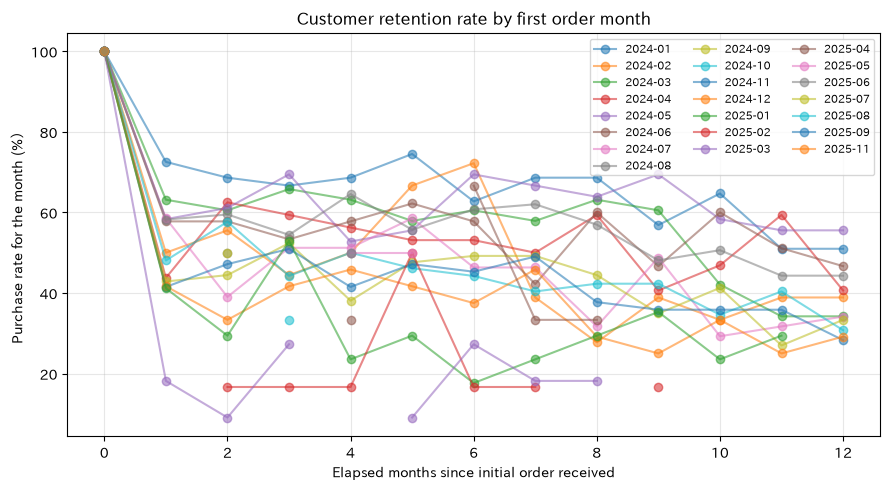
A significant drop from 100% in the first month to the following month is natural for B2B products that do not purchase monthly. The important thing is to compare cohorts within the same elapsed months. For example, if the acquisition month in the sixth month is weak in retention, further check acquisition channels, first-time purchase products, and whether there is technical follow-up during that period. Listing the cumulative repurchase rate together helps avoid misunderstandings about products with long purchasing cycles.

No.053: A/B Test — Measuring the Pure Effectiveness of Technical Consultation Meetings

Meaning in Practice

Looking only at the purchase rates of campaign participants, the influence of choosing customers who were originally highly interested is mixed. A/B tests that randomly divide candidates into intervention and control groups can be used for investment decisions before technical consultations or company-wide email campaigns.

Approach to Analysis and Modeling

The difference in purchase rates between the intervention and control groups (hat{p}_1-hat{p}_0) is estimated, and a 95% confidence interval is created from the standard error of the two-sample ratio. We will test the null hypothesis (H_0:p_1=p_0). However, not only statistical significance but also evaluation of whether gross profit increments exceed the cost of the initiative.

Check with Python

ab_rng = np.random.default_rng(SEED + 1)
n_ab = 1200
ab = pd.DataFrame({"treatment": ab_rng.binomial(1, 0.5, n_ab)})
ab["purchase"] = ab_rng.binomial(1, 0.105 + 0.038 * ab["treatment"])
rates = ab.groupby("treatment")["purchase"].agg(["mean", "sum", "count"])
p0, p1 = rates.loc[0, "mean"], rates.loc[1, "mean"]
diff = p1 - p0
se = np.sqrt(p0 * (1 - p0) / rates.loc[0, "count"] + p1 * (1 - p1) / rates.loc[1, "count"])
ci = (diff - 1.96 * se, diff + 1.96 * se)
z = diff / se
p_value = 2 * stats.norm.sf(abs(z))
display(rates.rename(index={0: "control group", 1: "intervention group"}))
print(f"Purchase rate difference: {diff:.1%} / 95%CI: [{ci[0]:.1%}, {ci[1]:.1%}] / pvalue: {p_value:.4f}")

fig, ax = plt.subplots(figsize=(7, 4))
ax.bar(["control group", "Technical Consultation Group"], [p0 * 100, p1 * 100], color=["#7f8c8d", "#2874a6"])
ax.errorbar(1, p1 * 100, yerr=1.96 * np.sqrt(p1 * (1-p1)/rates.loc[1, "count"]) * 100, color="black", capsize=5)
ax.set_title("A/BTest purchase rate comparison")
ax.set_xlabel("Distribution group")
ax.set_ylabel("Purchase rate (%）")
ax.grid(True, axis="y", alpha=0.3)
plt.tight_layout()
plt.show()

	mean	sum	count
treatment
control group	0.121	71	586
intervention group	0.168	103	614

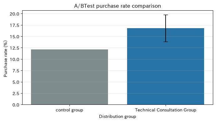
Purchase rate difference: 4.7% / 95% CI: [0.7%, 8.6%] / p-value: 0.0212

Reading the results

In point estimation, even if the purchase rate of the intervention group is high, if the confidence interval exceeds zero, it is read as “the current sample alone cannot determine the increment.” Rather than just discontinuing based on the presence of significant differences, we check expected incremental gross profit, consultation operation costs, and required sample size, and decide whether to conduct additional experiments or limited deployment. If you finish conveniently after checking the results midway, the number of Type 1 errors increases, so the timing of the judgment is decided in advance.

No.054: Customer Churn Analysis — Turning Signs of Order Stoppages into Prioritization

Meaning in Practice

Return analysis not only predicts “who is likely to leave,” but also helps sales focus on customers to check within a limited time. The definition is based on the product cycle, and here, a state where there are no orders within 120 days after the reference date is considered a renunciation.

Approach to Analysis and Modeling

From the purchase history up to the end of August 2025, we create Recency, Frequency, average unit price, and number of trading months, then set the 120-day divergence as the objective variable. Estimating probabilities with logistic regression and checking ranking ability with ROC-AUC. In actual operations, training and verification are separated in chronological order to avoid mixing in future information.

Check with Python

cutoff = pd.Timestamp("2025-08-31")
hist = orders[orders["order_date"] <= cutoff]
future = orders[(orders["order_date"] > cutoff) & (orders["order_date"] <= cutoff + pd.Timedelta(days=120))]
churn = hist.groupby("customer_id").agg(
    recency=("order_date", lambda s: (cutoff - s.max()).days),
    frequency=("order_id", "nunique"),
    avg_sales=("sales", "mean"),
    active_months=("order_date", lambda s: s.dt.to_period("M").nunique()),
).reset_index()
churn["churn"] = (~churn["customer_id"].isin(future["customer_id"])).astype(int)
features = ["recency", "frequency", "avg_sales", "active_months"]
X_train, X_test, y_train, y_test = train_test_split(churn[features], churn["churn"], test_size=0.3, random_state=SEED, stratify=churn["churn"])
churn_model = LogisticRegression(max_iter=2000).fit(X_train, y_train)
pred = churn_model.predict_proba(X_test)[:, 1]
print(f"Desertion rate: {churn['churn'].mean():.1%} / TestROC-AUC: {roc_auc_score(y_test, pred):.3f}")
coef = pd.Series(churn_model.coef_[0], index=features, name="coefficient")
display(coef.to_frame())

fig, ax = plt.subplots(figsize=(6, 5))
RocCurveDisplay.from_predictions(y_test, pred, ax=ax, name="defection model")
ax.set_title("Customer churn modelROCcurve")
ax.set_xlabel("false positive rate")
ax.set_ylabel("True positivity rate")
ax.grid(True, alpha=0.3)
plt.tight_layout()
plt.show()

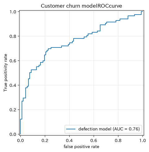
Bounce rate: 47.4% / Test ROC-AUC: 0.760

	coefficient
recency	0.017
frequency	0.014
avg_sales	-0.000
active_months	-0.038

Reading the results

ROC-AUC can be interpreted as the probability that randomly selected churned customers will be ranked higher risk than repeating customers. From the coefficient signs, we can see that the increase in Reninccy tends to work in the opposite direction. However, even if the predicted probability is high, intervention does not necessarily guarantee a recovery. Set the threshold for contact using the gross profit margin of top customers, the number of cases they can handle, and false positive costs.

No.055: Pareto/NBD — Capturing Variation in Purchase Frequency Using Probability Distributions

Meaning in Practice

It is common for a small number of customers to purchase multiple times while many customers purchase a small number of times, even in B2B. If you create a budget based only on average frequencies, you may mistakenly spread the influence of high-frequency customers to all customers. Pareto/NBD separates purchase generation and churn, and is a framework that considers future purchases across the entire customer base.

Approach to Analysis and Modeling

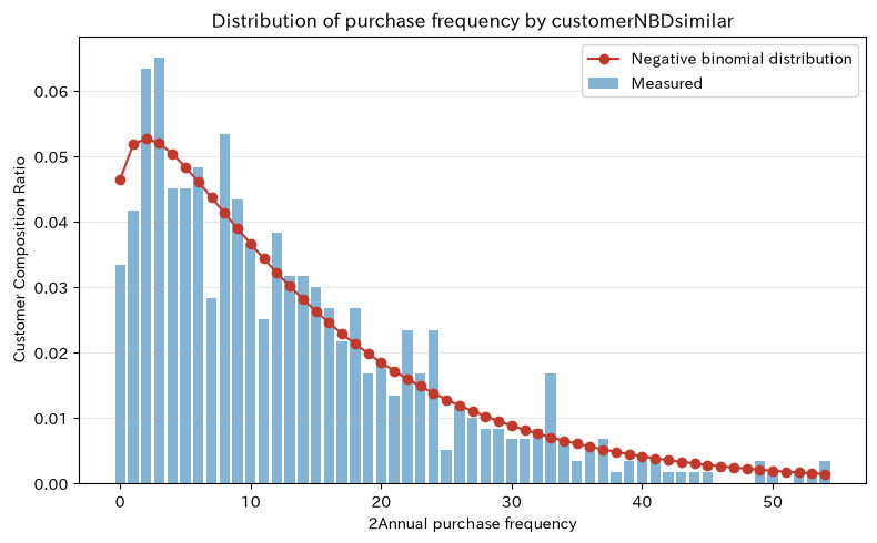
In Pareto/NBD, purchases during activity are assumed to follow the Poisson process of customer unique rate (lambda), the lambda as a Gamma distribution, the exit point as an exponential distribution, and churn rates also follow a Gamma distribution among customers. Here, as the first step, we apply the negative binomial distribution obtained from the Poisson-Gamma mixture using the moment method to confirm purchase heterogeneity. This is not a complete Pareto/NBD estimate, but a diagnosis of the number of purchases in the component.

Check with Python

purchase_counts = orders.groupby("customer_id")["order_id"].nunique().reindex(customers["customer_id"], fill_value=0)
mean_x, var_x = purchase_counts.mean(), purchase_counts.var()
shape_r = mean_x ** 2 / max(var_x - mean_x, 1e-9)
prob_p = shape_r / (shape_r + mean_x)
x = np.arange(0, int(purchase_counts.quantile(0.98)) + 1)
observed = purchase_counts.value_counts(normalize=True).reindex(x, fill_value=0)
fitted = stats.nbinom.pmf(x, shape_r, prob_p)
print(f"average: {mean_x:.2f}Return / disperse: {var_x:.2f} / GammaShape equivalent: {shape_r:.2f}")
display(pd.DataFrame({"Number of purchases": x[:10], "Measured Composition Ratio": observed.values[:10], "NBDEstimated composition ratio": fitted[:10]}))

fig, ax = plt.subplots(figsize=(8, 5))
ax.bar(x, observed.values, alpha=0.55, label="Measured")
ax.plot(x, fitted, color="#c0392b", marker="o", label="Negative binomial distribution")
ax.set_title("Distribution of purchase frequency by customerNBDsimilar")
ax.set_xlabel("2Annual purchase frequency")
ax.set_ylabel("Customer Composition Ratio")
ax.grid(True, axis="y", alpha=0.3)
ax.legend()
plt.tight_layout()
plt.show()

Average: 14.07 times / Dispersion: 177.36 / Gamma Shape Equivalent: 1.21

	Number of purchases	Measured Composition Ratio	NBDEstimated composition ratio
0	0	0.033	0.046
1	1	0.042	0.052
2	2	0.063	0.053
3	3	0.065	0.052
4	4	0.045	0.050
5	5	0.045	0.048
6	6	0.048	0.046
7	7	0.028	0.044
8	8	0.053	0.041
9	9	0.043	0.039

Reading the results

Overdispersion, where the variance is significantly above average, indicates that the purchase rate per customer is not uniform. If a negative binomial distribution can roughly represent hem length, you can visualize the risks of planning with only the “average customer.” When adopting Pareto/NBD in practice, it is important to examine the length of the observation window, the handling of contract customers, seasonality, and the definition of churn, and to confirm the reproducibility of future purchase volumes during the holding period.

No.056: BG/NBD — Estimating the survival probability of customers who haven’t bought recently

Meaning in Practice

Even with the same ‘no purchase in 6 months,’ the meaning differs between customers who used to buy monthly and those who only once a year. BG/NBD combines purchase frequency, last purchase point, and observation period, representing the probability that the product is still tradable.

Approach to Analysis and Modeling

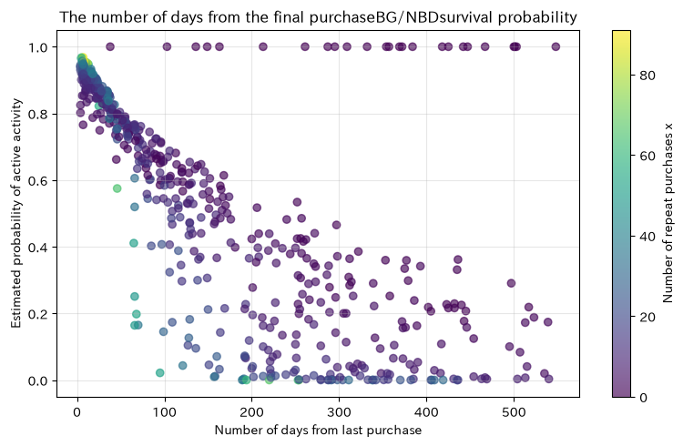
In BG/NBD, we assume a Gamma distribution for purchase rate and a Beta distribution for churn probability after each purchase. Let the number of repeated purchases be (x), the period from the first to the last purchase be (t_x), and the period from the first to the end of observation (T). The survival probability of (x>0) can be expressed as follows.

$$P(\mathrm{alive})=\left[1+\frac{a}{b+x-1}\left(\frac{\alpha+T}{\alpha+t_x}\right)^{r+x}\right]^{-1}$$

Here, we use example parameters to clarify the behavior. In actual testing, the most likely estimate is performed and calibrated according to the holding period for the time series.

Check with Python

bg = orders.groupby("customer_id").agg(first=("order_date", "min"), last=("order_date", "max"), n=("order_id", "nunique")).reset_index()
bg["x"] = (bg["n"] - 1).clip(lower=0)
bg["t_x"] = (bg["last"] - bg["first"]).dt.days / 30.44
bg["T"] = (ANALYSIS_END - bg["first"]).dt.days / 30.44
r, alpha, a, b = 0.9, 5.0, 1.4, 3.8
ratio = (alpha + bg["T"]) / (alpha + bg["t_x"])
bg["p_alive"] = np.where(bg["x"] > 0, 1 / (1 + a / (b + bg["x"] - 1) * ratio ** (r + bg["x"])), 1.0)
display(bg.sort_values("p_alive").head(10)[["customer_id", "x", "t_x", "T", "p_alive"]])

fig, ax = plt.subplots(figsize=(8, 5))
scatter = ax.scatter((ANALYSIS_END - bg["last"]).dt.days, bg["p_alive"], c=bg["x"], cmap="viridis", alpha=0.65)
ax.set_title("The number of days from the final purchaseBG/NBDsurvival probability")
ax.set_xlabel("Number of days from last purchase")
ax.set_ylabel("Estimated probability of active activity")
ax.grid(True, alpha=0.3)
fig.colorbar(scatter, ax=ax, label="Number of repeat purchases x")
plt.tight_layout()
plt.show()

	customer_id	x	t_x	T	p_alive
292	C0301	73	15.637	23.982	0.000
272	C0280	31	7.884	21.649	0.000
77	C0080	39	10.710	21.813	0.000
27	C0029	33	10.480	23.817	0.000
435	C0449	62	15.670	23.982	0.000
391	C0405	67	16.491	23.719	0.000
575	C0596	28	9.823	23.259	0.000
502	C0519	24	8.706	20.861	0.000
202	C0210	22	9.658	23.949	0.000
374	C0386	60	17.181	23.555	0.000

Reading the results

Even if the number of days since the last purchase is the same, survival probabilities vary depending on the number of repeat purchases and the observation period. In sales lists, you can add this probability to dormant RFM candidates and prioritize customers with high historical value but a sharp drop in survival probability. For businesses or subscriptions where contract termination is explicitly stated, assumptions may not match, so comparisons are made with rule-based or alternative lifetime models.

No.057: CLV — Considering the Upper Limit of Customer Investment from Future Gross Margin

Meaning in Practice

Even if sales are the same, differences in gross profit margin, retention rate, and response costs will result in different customer value. CLV (Customer Lifetime Value) is an indicator used to align investment amounts such as visits, technical support, and discounts with future gross profit.

Approach to Analysis and Modeling

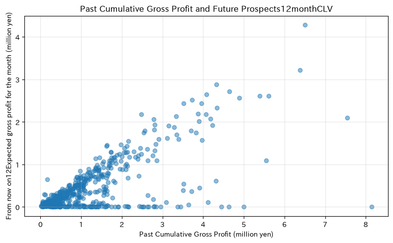
Simply put, the expected gross profit for the future (H) period is (CLV_i=\sum_{h=1}^{H} E[N_{ih}]\bar{m}_i/(1+d)^h-C_i). Here, we combine the survival probability of BG/NBD, the annual purchase rate in the past, and the average gross profit margin on orders to calculate the expected gross profit over one year. Since taxes, fixed costs, and acquisition costs are not included, it is a “provisional CLV based on gross margin.”

Check with Python

value = orders.groupby("customer_id").agg(total_gp=("gross_profit", "sum"), avg_gp=("gross_profit", "mean"), orders=("order_id", "nunique"), first=("order_date", "min"))
value["observed_years"] = ((ANALYSIS_END - value["first"]).dt.days / 365.25).clip(lower=0.25)
value["annual_rate"] = value["orders"] / value["observed_years"]
value = value.join(bg.set_index("customer_id")["p_alive"])
value["expected_orders_12m"] = value["annual_rate"] * value["p_alive"]
value["clv_12m"] = value["expected_orders_12m"] * value["avg_gp"] / 1.05
display(value.sort_values("clv_12m", ascending=False).head(10)[["p_alive", "annual_rate", "avg_gp", "expected_orders_12m", "clv_12m"]])

fig, ax = plt.subplots(figsize=(8, 5))
ax.scatter(value["total_gp"] / 1e6, value["clv_12m"] / 1e6, alpha=0.5)
ax.set_title("Past Cumulative Gross Profit and Future Prospects12monthCLV")
ax.set_xlabel("Past Cumulative Gross Profit (million yen)")
ax.set_ylabel("From now on12Expected gross profit for the month (million yen)")
ax.grid(True, alpha=0.3)
plt.tight_layout()
plt.show()

	p_alive	annual_rate	avg_gp	expected_orders_12m	clv_12m
customer_id
C0496	0.956	66.541	70,636.072	63.614	4,279,497.524
C0285	0.968	48.737	71,746.488	47.177	3,223,577.292
C0264	0.851	33.652	105,616.127	28.638	2,880,606.246
C0464	0.967	38.614	76,228.042	37.348	2,711,395.895
C0016	0.946	40.264	72,934.324	38.098	2,646,327.135
C0155	0.873	26.256	119,761.607	22.910	2,613,120.129
C0488	0.950	40.526	71,052.960	38.515	2,606,289.993
C0163	0.906	25.483	116,543.478	23.075	2,561,135.158
C0506	0.943	25.605	109,558.505	24.155	2,520,416.992
C0591	0.949	24.532	110,053.506	23.287	2,440,755.352

Reading the results

Even if past gross profit is high, if survival probability is low, future CLV will be low. Conversely, even if your trading history is short, if you have high frequency and high gross margin, you can be a target for development. CLV is not a score that cuts off customers, but information that designs service levels and acquisition cost caps. In production, we reflect product-specific gross profit, returns, sales hours, contract renewals, and forecast uncertainties, sharing them across ranges rather than single values.

No.058: Market Basket Analysis — Finding Proposal Combinations from Simultaneous Purchases

Meaning in Practice

By understanding which parts will be purchased together within an order, you can use it to propose accessories during quotes, design maintenance kits, and improve the routing of your e-commerce screen. Since simple simultaneous transactions alone can rank high for popular products, we see connections beyond just chance with lift.

Approach to Analysis and Modeling

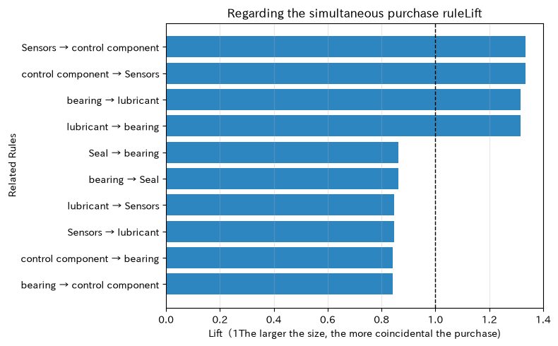
For products (A, B), support is (P(A\cap B)), confidence is (P(B| A)), lift is (P(A\cap B)/(P(A)P(B))). If lift exceeds 1, it indicates more simultaneous purchases than in independent cases. However, this is not an indicator representing incremental effects from causality or suggestions.

Check with Python

basket = pd.crosstab(order_lines["order_id"], order_lines["product"]).gt(0)
rules = []
for a, b in itertools.permutations(basket.columns, 2):
    support_a = basket[a].mean()
    support_b = basket[b].mean()
    support_ab = (basket[a] & basket[b]).mean()
    confidence = support_ab / support_a
    lift = confidence / support_b
    rules.append((a, b, support_ab, confidence, lift))
rules = pd.DataFrame(rules, columns=["previous case", "Subsequent case", "support", "confidence", "lift"])
top_rules = rules.query("support >= 0.03").sort_values(["lift", "support"], ascending=False).head(10)
display(top_rules)

fig, ax = plt.subplots(figsize=(8, 5))
plot_rules = top_rules.sort_values("lift")
labels = plot_rules["previous case"] + " → " + plot_rules["Subsequent case"]
ax.barh(labels, plot_rules["lift"], color="#2e86c1")
ax.axvline(1.0, color="black", linestyle="--", linewidth=1)
ax.set_title("Regarding the simultaneous purchase ruleLift")
ax.set_xlabel("Lift（1The larger the size, the more coincidental the purchase)")
ax.set_ylabel("Related Rules")
ax.grid(True, axis="x", alpha=0.3)
plt.tight_layout()
plt.show()

	previous case	Subsequent case	support	confidence	lift
7	Sensors	control component	0.177	0.526	1.334
16	control component	Sensors	0.177	0.448	1.334
29	bearing	lubricant	0.247	0.572	1.315
24	lubricant	bearing	0.247	0.568	1.315
4	Seal	bearing	0.133	0.373	0.862
25	bearing	Seal	0.133	0.307	0.862
8	Sensors	lubricant	0.124	0.369	0.848
21	lubricant	Sensors	0.124	0.285	0.848
19	control component	bearing	0.143	0.363	0.841
28	bearing	control component	0.143	0.332	0.841

Reading the results

High-lift rules such as “bearing → lubricants” and “sensors → control components” serve as hypotheses for estimate checks and set proposals. Confidence has a direction, and its value differs between A to B and B to A. To avoid accidental low support or falsification due to product line, season, or distributor inventory, we check reproducibility by period and measure incremental gross profit through small-scale proposal experiments.

No.059: Recommendation System — Creating the Next Product Candidate by Customer

Meaning in Practice

Basket analysis shows the overall mix, while recommendations change candidates based on the customer’s purchase history. In sales support, using it as a “second-best product candidate” where the person in charge can check the reason for the proposal is easier to implement than automatic submission.

Approach to Analysis and Modeling

Create a customer × product purchase count row (X) and calculate the cosine similarity between product vectors (s_{jk} = x_j^Tx_k/(|x_j||x_k|)). Adds up the similarity between products customers have already purchased and ranks unpurchased items. Popularity bias, cold starts, and explainability are the main operational challenges.

Check with Python

customer_item = pd.crosstab(order_lines["customer_id"], order_lines["product"])
similarity = pd.DataFrame(cosine_similarity(customer_item.T), index=customer_item.columns, columns=customer_item.columns)
similarity = similarity.mask(np.eye(len(similarity), dtype=bool), 0.0)

def recommend(customer_id, n=3):
    history = customer_item.loc[customer_id]
    scores = similarity.dot(np.log1p(history))
    scores[history > 0] = -np.inf
    return scores.nlargest(n)

product_variety = customer_item.gt(0).sum(axis=1)
candidate_customers = product_variety[product_variety.between(1, 3)].index
target_customer = candidate_customers[len(candidate_customers) // 2]
history = customer_item.loc[target_customer]
result = pd.DataFrame({"Number of purchases": history[history > 0], "Classification": "Purchased"})
recs = recommend(target_customer)
print("Target Customers:", target_customer)
display(result)
display(recs.rename("Recommendation Score").to_frame())

fig, ax = plt.subplots(figsize=(7, 5))
im = ax.imshow(similarity, cmap="Blues", vmin=0, vmax=1)
ax.set_xticks(range(len(similarity)), similarity.columns, rotation=45, ha="right")
ax.set_yticks(range(len(similarity)), similarity.index)
ax.set_title("Cosine similarity between products")
ax.set_xlabel("Product Categories")
ax.set_ylabel("Product Categories")
ax.grid(False)
fig.colorbar(im, ax=ax, label="similarity")
plt.tight_layout()
plt.show()

Target Customer: C0250

	Number of purchases	Classification
product
Seal	1	Purchased
Sensors	2	Purchased
Maintenance Kit	1	Purchased

	Recommendation Score
product
control component	2.336
bearing	2.327
lubricant	2.320

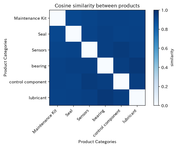
Reading the results

Recommendation results indicate candidates for “unpurchased categories used by customers with similar purchasing behavior.” Do not automatically propose solutions while ignoring compatibility, existing equipment, agency contracts, inventory, or legal regulations. By recording the reasons for hiring or rejecting the representative, it becomes training data that improves not only recommendation accuracy but also negotiation rates, incremental gross margin, and inappropriate proposal rates.

No.060: Uplift Modeling — Finding Customers Who Change Their Behavior Through Initiatives

Meaning in Practice

Even if you focus your efforts on customers with a high purchase probability, those customers may have bought without any initiative. Uplift Modeling estimates the difference in response between intervention and non-intervention for each customer, allocating limited sales hours to the segment where actions change through engagement.

Approach to Analysis and Modeling

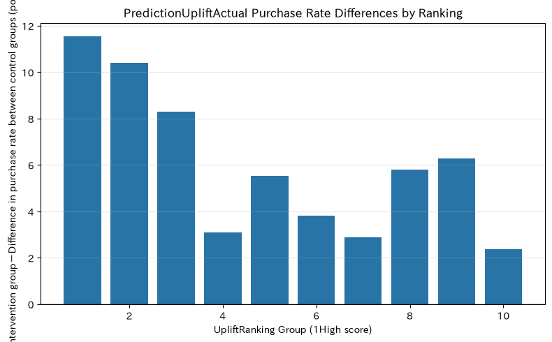
For customer features (X), the individual effect is defined as (au(X) = P(Y = 1| T=1,X)-P(Y=1| T = 0, X)). Here, randomly assigned data is trained using two logistic regressions (T-learners) for intervention and control groups. Since causal effects at the individual level cannot be observed, validity is evaluated using measured increments by ranking.

Check with Python

up_rng = np.random.default_rng(SEED + 2)
n_up = 5000
uplift_data = pd.DataFrame({
    "recency": up_rng.gamma(2.2, 55, n_up),
    "frequency": up_rng.poisson(5, n_up),
    "margin": up_rng.lognormal(np.log(60_000), 0.55, n_up),
    "treatment": up_rng.binomial(1, 0.5, n_up),
})
base_logit = -2.4 - 0.006 * uplift_data["recency"] + 0.10 * uplift_data["frequency"]
true_uplift_logit = 0.9 * ((uplift_data["recency"] > 45) & (uplift_data["recency"] < 170)) - 0.35 * (uplift_data["frequency"] >= 8)
p = 1 / (1 + np.exp(-(base_logit + uplift_data["treatment"] * true_uplift_logit)))
uplift_data["purchase"] = up_rng.binomial(1, p)
features_up = ["recency", "frequency", "margin"]

model_t = LogisticRegression(max_iter=2000).fit(uplift_data.loc[uplift_data.treatment == 1, features_up], uplift_data.loc[uplift_data.treatment == 1, "purchase"])
model_c = LogisticRegression(max_iter=2000).fit(uplift_data.loc[uplift_data.treatment == 0, features_up], uplift_data.loc[uplift_data.treatment == 0, "purchase"])
uplift_data["uplift_score"] = model_t.predict_proba(uplift_data[features_up])[:, 1] - model_c.predict_proba(uplift_data[features_up])[:, 1]
uplift_data["decile"] = pd.qcut(uplift_data["uplift_score"].rank(method="first"), 10, labels=False)
evaluation = uplift_data.groupby(["decile", "treatment"])["purchase"].mean().unstack()
evaluation["observed_uplift"] = evaluation[1] - evaluation[0]
evaluation = evaluation.sort_index(ascending=False)
display(evaluation.rename(columns={0: "Control group purchase rate", 1: "Intervention Group Purchase Rate", "observed_uplift": "MeasuredUplift"}))

fig, ax = plt.subplots(figsize=(8, 5))
ax.bar(range(1, 11), evaluation["observed_uplift"] * 100, color=np.where(evaluation["observed_uplift"] >= 0, "#2874a6", "#c0392b"))
ax.axhline(0, color="black", linewidth=1)
ax.set_title("PredictionUpliftActual Purchase Rate Differences by Ranking")
ax.set_xlabel("UpliftRanking Group (1High score)")
ax.set_ylabel("intervention group－Difference in purchase rate between control groups (points)")
ax.grid(True, axis="y", alpha=0.3)
plt.tight_layout()
plt.show()

treatment	Control group purchase rate	Intervention Group Purchase Rate	MeasuredUplift
decile
9	0.074	0.189	0.115
8	0.048	0.152	0.104
7	0.055	0.137	0.083
6	0.094	0.125	0.031
5	0.061	0.117	0.055
4	0.060	0.098	0.038
3	0.096	0.125	0.029
2	0.076	0.134	0.058
1	0.048	0.111	0.063
0	0.017	0.041	0.024

Reading the results

If there is a large difference in actual purchase rates among high-scoring groups, there is room to narrow down the target beyond all customer distributions. The negative uplift group is excluded from the list because the measures can be counterproductive. However, the results of training and evaluating with the same data are optimistic. In production, randomization is maintained, and verification data segmented by time or customer are used to evaluate Qini curves, incremental gross margin, and contact costs.

Practical Implications Seen Through Target Exercise

The 10 themes are not independent analyses but are connected as follows: We organize the current situation using RFMs and cohorts, and estimate future purchasing and dormancy risks using Pareto/NBD, BG/NBD, and divergence models. We set a cap on the handling fee with CLV, and create proposals through basket analysis and recommendations. Finally, use A/B testing and uplift modeling to verify whether the proposal truly changed behavior.

In manufacturing, not only forecasting accuracy but also connection with supply capacity is crucial. Even if you offer specific products all at once to high-uplift customers, insufficient inventory or production capacity can harm customer experience and profits. It is necessary to design KPIs that allow confirmation of the number of target initiatives, expected demand, gross profit, and supply constraints in the same meeting.

What is necessary for practical implementation

1. IDand maintenance at that point: Align customer integrated IDs and the timing of orders, returns, quotations, and contact histories
2. Definition agreement: Unified purchasing, defection, gross profit, policy expenses, and customer units across sales, accounting, and IT
3. Verification Design: Use only information prior to the forecast period to secure retention periods and randomized control groups
4. Implementation of Business Constraints: Reflect equipment compatibility, inventory, number of cases you can handle, and agency contracts in your recommendations and selection
5. Decision-makingKPI: In addition to AUC and accuracy, we track incremental gross profit, negotiation rate, inappropriate proposal rate, and supply fulfillment rate.
6. Improvement from small-scale operations: Conduct tests in a way that allows the person in charge to verify the reasons, and carry the results back to the next learning session

A model is not made once and is not finished. When purchasing cycles, product mix, pricing, and sales operations change, features and thresholds also change. It is important to design monthly data quality monitoring and quarterly effectiveness verification as your responsibilities.

Conclusion

From No.051 to No.060, we used fictitious data from industrial parts manufacturers to reinterpret customers not only by “past sales” but also from the perspectives of retention, turnover, survival probability, future gross profit, mergers, and behavioral changes due to policies.

• RFM cohorts use a common language to address current situations and changes in customer relationships
• Pareto/NBD, BG/NBD, and Divergence Analysis probabilistically treats differences in purchase frequency and dormancy
• CLV links future operating and service investments to gross profit.
• Basket analysis and recommendations create proposal candidates and complete them based on operational constraints and the judgment of the person in charge.
• A/B testing and uplift modeling evaluate “customers who have changed through initiatives” rather than “responsive customers.”

The ultimate goal is not to introduce advanced models, but to build a decision-making cycle about who to propose what to and how to learn from the results.

Consultations for Corporations

At Surikoubo, we handle everything from problem organization to supporting the design of customer data platforms in manufacturing, building defection, CLV, and demand forecasting models, experimental design of sales strategies, and decision support that connects recommendation results with production and inventory constraints. You can consult with us from the stage where you have an order history but don’t translate into measures or want to embed analysis results in the sales field.

📩 Contact Us: surikobo.co.jp/contact
Please feel free to consult us first.