Balancing Profit and Supply Responsibility Under Uncertainty: 10 Key Exercises on Manufacturing Decision Science

This article focuses on a fictional industrial sensor manufacturer and treats Maximizing expected value, minimizing risk, utility theory, decision trees, Bayesian decision-making,MDP、POMDPScenario analysis, sensitivity analysis, robust optimization as a continuous process of decision-making.

With equipment expansion, outsourcing, maintenance, procurement, and production allocation, future demand and failures cannot be fully predicted. Therefore, rather than relying on a single prediction value, we consider possible scenarios, probabilities, losses, unobservable conditions, and resistance to the unexpected separately. The published data is generated in Python and does not depend on external data.

[!NOTE] This material is a notebook previously used by Surikoubo (or personally by the representative, Kazuyama), and has been reconstructed, edited, and published with the company’s permission.
All data listed is fictional and has no relation whatsoever to real companies, factories, or figures.

Introduction: Practical Challenges in Manufacturing Covered in This Article

The target companies produce industrial sensors with large fluctuations in orders. When demand is strong, expanding facilities generates profits, but when demand is weak, fixed costs remain. Outsourcing increases the ability to keep up with demand, but also leads to fluctuations in unit prices and delivery times. Also, the deterioration of equipment is not fully visible, and disruptions at suppliers or deterioration in processing time can occur.

The purpose of this article is not to “choose the most likely prediction.” It means clearly stating Options, uncertain conditions, outcomes, value criteria, information updates and creating a situation where decision-makers can explain their reasons for judgment and the conditions for review.

Common situations on site

• Capital investment is decided solely based on average demand forecasts, overlooking fixed cost burdens during downward trends.
• Although a plan with high expected profits is adopted, unacceptable losses due to cash flow occur
• Sensor alarms are regarded as confirmed failures, leading to an increase in overmaintenance due to false alarms.
• Even when new information arrives, discussions continue in planning meetings based on old probabilities and assumptions
• Considering exchange rates, material costs, and logistics disruptions separately, without comparing composite scenarios.
• Only the numbers for the optimal solution are shared, and it’s unclear which assumptions change to reverse the conclusion

What these have in common is that uncertainty is pushed into a single safety factor, making the decision-making structure invisible.

Why is this issue so difficult to judge?

Looking at the same data, shareholders may focus on expected profits, plant managers may focus on supply halts, and finance departments may focus on maximum losses. Furthermore, demand, equipment status, and procurement environments change over time, and probabilities are updated with additional information.

Therefore, a single KPI alone is not enough. This article lists expected value, downside risk, certainty equivalence, value of information, future costs, post-event probability, worst-case scenario, and boundaries where conclusions are reversed. Models do not automatically justify decisions; they use them as Tools that enable auditing assumptions and trade-offs.

Overview of Exercise covered this time

No.	Theme	Main Questions	Main Outputs
071	Maximizing expected value	Which option offers the highest average profit after considering probability?	Expected Profits, Lost Opportunities
072	Risk Minimization	How much to suppress bad outcomes?	Lower quantr, CVaR
073	Utility theory	How to Reflect Risk Tolerance in Choices	certainty equivalent
074	decision tree	Is it worth investing?	Branch-by-branch judgment, expected value
075	Bayesian Decision-Making	How to update decisions using demand signals	Post Hi Facto Probability, Recommended Proposal
076	MDP	When to carry out maintenance while monitoring the condition of the equipment	State-specific measures and future costs
077	POMDP	How to judge when the deterioration state is not directly visible?	Belief Probability, Inspection Threshold
078	scenario analysis	Can procurement proposals withstand complex external environments?	Profitability by scenario
079	sensitivity analysis	On what assumptions can the conclusion be reversed?	switching boundary
080	Robust optimization	What are the feasible plans even if processing time deteriorates?	Robust Production Allocation

Preparing the Python environment

NumPy is used for numerical computation and random number generation, pandas for decision tables, and matplotlib for visualization. Random number seeds are fixed to 42. japanize_matplotlib loads to stabilize the Japanese display within the graph.

import platform

import matplotlib.pyplot as plt
import numpy as np
import pandas as pd
import japanize_matplotlib
from IPython.display import display

SEED = 42
rng = np.random.default_rng(SEED)
pd.set_option("display.max_columns", 20)
pd.set_option("display.float_format", lambda x: f"{x:,.2f}")

print(f"Python: {platform.python_version()}")
print(f"NumPy: {np.__version__} / pandas: {pd.__version__}")
print(f"random numberseed: {SEED}")

Python: 3.13.1
NumPy: 2.5.1 / pandas: 3.0.3
Random seed: 42

Creation of Fictional Data

For the next fiscal year, we will compare three capability policies: “Continuing existing equipment,” “Outsourcing for flexibility,” and “Strengthening facilities.” Demand levels are bearish, standard, and bullish, with profit units in millions of yen. Profit is defined as the marginal profit for decision-making, which is the deduction of variable costs, outsourcing costs, fixed costs, and stockout penalties from sales.

In practice, probabilities and profits are not determined by the same person alone; sales, production, procurement, and finance all contribute to the evidence. Also, unless the expense category included in ‘profit’ and the evaluation period are aligned, the proposals cannot be fairly compared.

states = ["bearish demand", "standard requirement", "Bullish demand"]
plans = ["Continuing existing equipment", "Flexibility through outsourcing", "Facility Enhancement"]
probability = pd.Series([0.25, 0.50, 0.25], index=states, name="prior probability")
profit = pd.DataFrame(
    [[42, 58, 64], [35, 66, 86], [10, 70, 118]],
    index=plans,
    columns=states,
)

likelihood = pd.DataFrame(
    [[0.65, 0.25, 0.10], [0.25, 0.50, 0.25], [0.10, 0.25, 0.65]],
    index=["Weak Order Signals", "Normal signal", "Strong Order Signals"],
    columns=states,
)

print("Decision-making profit (million yen)")
display(profit)
print("Prior probability of demand conditions")
display(probability.to_frame().T)
print("Probability of Observing Order Signals in Each Demand Condition")
display(likelihood)

Decision-making profit (million yen)

	bearish demand	standard requirement	Bullish demand
Continuing existing equipment	42	58	64
Flexibility through outsourcing	35	66	86
Facility Enhancement	10	70	118

Prior probability of demand conditions

	bearish demand	standard requirement	Bullish demand
prior probability	0.25	0.50	0.25

Probability of Observing Order Signals in Each Demand Condition

	bearish demand	standard requirement	Bullish demand
Weak Order Signals	0.65	0.25	0.10
Normal signal	0.25	0.50	0.25
Strong Order Signals	0.10	0.25	0.65

No.071: Maximizing Expected Value — Choosing Capability Policies Based on Demand Probability

Meaning in Practice

Maximizing expected value serves as a criterion for repeatable decisions and for investment deals that can diversify risk across the entire company. Rather than comparing equipment expansion, outsourcing, and maintaining the status quo solely by the “most likely demand,” all conditions are probably-weighted.

Approach to Analysis and Modeling

The expected benefit for action $a$, state $s$, profit $V(a,s)$, and state probability $p(s)$ is

$\mathbb{E}[V(a,S)]=\sum_s p(s)V(a,s)$

That’s right. Furthermore, the difference between the best profit after the fact in each state is expressed as a regret $R(a,s)=\max_{a'}V(a',s)-V(a,s)$. For proposals with similar expected values, average regret can also be a factor in decision-making.

Check with Python

expected_profit = profit.mul(probability, axis=1).sum(axis=1)
regret = profit.max(axis=0) - profit
decision_071 = pd.DataFrame({
    "Expected Profit (million yen)": expected_profit,
    "Expectant Regret (million yen)": regret.mul(probability, axis=1).sum(axis=1),
}).sort_values("Expected Profit (million yen)", ascending=False)
display(decision_071)

ax = decision_071["Expected Profit (million yen)"].sort_values().plot(
    kind="barh", color=["#9ecae1", "#6baed6", "#2171b5"], figsize=(8, 4)
)
ax.set_title("Expected Returns by Capability Policy")
ax.set_xlabel("Expected Profit (million yen)")
ax.set_ylabel("Capability Policy")
ax.grid(axis="x", alpha=0.3)
plt.tight_layout()
plt.show()

print(f"Recommended Proposals Based on Expected Values: {expected_profit.idxmax()}")

	Expected Profit (million yen)	Expectant Regret (million yen)
Facility Enhancement	67.00	8.00
Flexibility through outsourcing	63.25	11.75
Continuing existing equipment	55.50	19.50

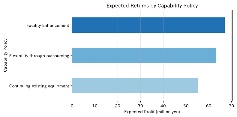
Recommended Expected Value Standard: Upgrade Facilities

Reading the results

Under the preliminary probability model, the expected profit from “facility expansion” is the maximum. However, with bearish demand, profits can drop to 10 million yen, and the gap with the best option after the fact becomes larger. Expectations are based on long-term averages and do not automatically reflect single-year funding constraints or supply responsibilities. In investment decisions, it is presented together with downside risk of the next exercise.

No.072: Minimizing Risk — Measuring Not Just Average Profit, but Downside

Meaning in Practice

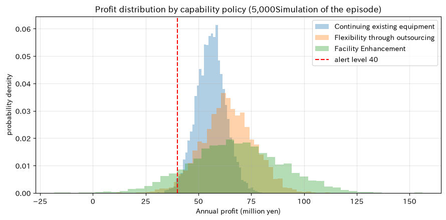
Even if the average profit is high, a plan that incurs a large loss at certain probabilities may not meet borrowing conditions or employment retention constraints. Here, a hypothetical fiscal year is generated including demand error, startup delays, and fluctuations in outsourced unit prices.

Approach to Analysis and Modeling

The 5% percentile of profit $Y$ represents a “bad level about one in twenty times.” The lower CVaR, which is the average of the lower 10%,

$\mathrm{CVaR}_{10\%}^{\mathrm{lower}}(Y)=\mathbb{E}[Y\mid Y\le q_{0.1}(Y)]$

This is how it is calculated. Since it is profit, a higher value is desirable, and note that the sign is opposite to the loss expression CVaR.

Check with Python

risk_rng = np.random.default_rng(SEED)
n_sim = 5000
simulated_profit = pd.DataFrame({
    "Continuing existing equipment": risk_rng.normal(56, 7, n_sim),
    "Flexibility through outsourcing": risk_rng.normal(64, 12, n_sim),
    "Facility Enhancement": risk_rng.normal(69, 21, n_sim)
        - risk_rng.binomial(1, 0.05, n_sim) * risk_rng.uniform(12, 28, n_sim),
})

risk_rows = []
for plan in simulated_profit:
    values = simulated_profit[plan]
    q10 = values.quantile(0.10)
    risk_rows.append({
        "Capability Policy": plan,
        "average_profit": values.mean(),
        "5%quantile": values.quantile(0.05),
        "BelowCVaR 10%": values[values <= q10].mean(),
        "interest40Less than probability": (values < 40).mean(),
    })
risk_table = pd.DataFrame(risk_rows).set_index("Capability Policy")
display(risk_table)

fig, ax = plt.subplots(figsize=(9, 4.5))
for plan in simulated_profit:
    ax.hist(simulated_profit[plan], bins=45, alpha=0.35, density=True, label=plan)
ax.axvline(40, color="red", linestyle="--", label="alert level 40")
ax.set_title("Profit distribution by capability policy (5,000Simulation of the episode)")
ax.set_xlabel("Annual profit (million yen)")
ax.set_ylabel("probability density")
ax.grid(alpha=0.3)
ax.legend()
plt.tight_layout()
plt.show()

	average_profit	5%quantile	BelowCVaR 10%	interest40Less than probability
Capability Policy
Continuing existing equipment	55.86	44.19	43.50	0.01
Flexibility through outsourcing	63.99	44.07	42.66	0.02
Facility Enhancement	67.76	32.93	30.47	0.10

Reading the results

While facility expansion has a higher average profit, the distribution is long, and the probability of profits below 40 million yen is also high. The existing equipment proposal has a low upward swing but a good downward CVaR. Management meetings can clearly state that the “plan maximizes average profit” and the “one that can endure tough years” are different. Analysts do not set the minimum allowable limits; instead, they set them based on financial constraints and business continuity conditions.

No.073: Utility Theory — Converting Risk Tolerance into Certainty Equivalence

Meaning in Practice

Even with the same profit distribution, companies with financial capacity and those needing to avoid single-year losses make different choices. Utility theory reduces the difference not just to the term “cautious or proactive,” but to formulas.

Approach to Analysis and Modeling

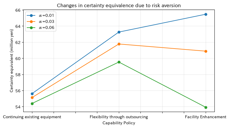
We use the exponential utility $U(y)=-e^{-\alpha y}$, which $\alpha>0$ absolute risk aversion. Certainty Equivalent (CE) is

$\mathrm{CE}=-\frac{1}{\alpha}\log\left(\mathbb{E}[e^{-\alpha Y}]\right)$

That’s right. This means “uncertain profit $Y$ certain profit with the same utility.” The larger the $\alpha$, the stronger the downward movement is disliked.

Check with Python

alphas = [0.01, 0.03, 0.06]
ce = pd.DataFrame(index=simulated_profit.columns)
for alpha in alphas:
    ce[f"α={alpha:.02f}"] = [
        -np.log(np.mean(np.exp(-alpha * simulated_profit[plan]))) / alpha
        for plan in simulated_profit
    ]
display(ce)

ax = ce.plot(marker="o", figsize=(8, 4.5))
ax.set_title("Changes in certainty equivalence due to risk aversion")
ax.set_xlabel("Capability Policy")
ax.set_ylabel("Certainty equivalent (million yen)")
ax.grid(alpha=0.3)
plt.xticks(rotation=0)
plt.tight_layout()
plt.show()

	α=0.01	α=0.03	α=0.06
Continuing existing equipment	55.62	55.13	54.39
Flexibility through outsourcing	63.25	61.77	59.53
Facility Enhancement	65.46	60.88	53.93

Reading the results

When risk aversion is low, proposals with higher average profits are more likely to be evaluated, while when risk aversion is increased, the certainty equivalence of highly varied facility expansion proposals decreases. The important thing is not to arbitrarily choose $\alpha$. Check the consistency with past investment choices, allowable losses, and financial capacity, and line up multiple $\alpha$ to assess the stability of the conclusion.

No.074: Decision Tree — Measuring Investment Value After Market Testing

Meaning in Practice

Instead of making a large investment immediately, you may be able to gather information through test sales to early customers or prototyping lines before choosing the scale. The decision tree clearly states the order of “invest/don’t” and “see the results and invest/don’t.”

Approach to Analysis and Modeling

Calculate backward from ending profit. The decision node takes the maximum value, while the probability node takes the expected value Rollback If we set the testing cost as $C$, the value of an informed strategy is

$V_{\mathrm{test}}=-C+\sum_z P(z)\max_a\mathbb{E}[V(a,S)\mid z]$

That’s right. The comparison is the value of choosing the best course of action immediately without information.

Check with Python

pilot = pd.DataFrame({
    "Test Results": ["favorable impression", "cautious reaction"],
    "Probability of occurrence": [0.55, 0.45],
    "Success Probability of Full-scale Enhancement": [0.75, 0.30],
})
expand_success, expand_failure = 105, 5
small_scale_profit, test_cost = 52, 2
pilot["Conditional expected profit from enhancement"] = (
    pilot["Success Probability of Full-scale Enhancement"] * expand_success
    + (1 - pilot["Success Probability of Full-scale Enhancement"]) * expand_failure
)
pilot["Selection after result observation"] = np.where(
    pilot["Conditional expected profit from enhancement"] > small_scale_profit, "Full-scale Enhancement", "Small-scale improvements"
)
pilot["Value after selection"] = pilot[["Conditional expected profit from enhancement"]].iloc[:, 0].clip(lower=small_scale_profit)

prior_success = (pilot["Probability of occurrence"] * pilot["Success Probability of Full-scale Enhancement"]).sum()
no_test_value = max(
    prior_success * expand_success + (1 - prior_success) * expand_failure,
    small_scale_profit,
)
test_value = (pilot["Probability of occurrence"] * pilot["Value after selection"]).sum() - test_cost
display(pilot)
display(pd.DataFrame({
    "Strategy": ["Immediately implement the best plan.", "Divergence After Market Testing"],
    "Expected value (million yen)": [no_test_value, test_value],
}).set_index("Strategy"))

ax = pilot.set_index("Test Results")[["Conditional expected profit from enhancement", "Value after selection"]].plot(
    kind="bar", figsize=(8, 4.5), color=["#9ecae1", "#2171b5"]
)
ax.axhline(small_scale_profit, color="red", linestyle="--", label="Small-scale improvements")
ax.set_title("Conditional value per market test result")
ax.set_xlabel("Market Test Results")
ax.set_ylabel("Profit (million yen)")
ax.grid(axis="y", alpha=0.3)
ax.legend()
plt.xticks(rotation=0)
plt.tight_layout()
plt.show()

	Test Results	Probability of occurrence	Success Probability of Full-scale Enhancement	Conditional expected profit from enhancement	Selection after result observation	Value after selection
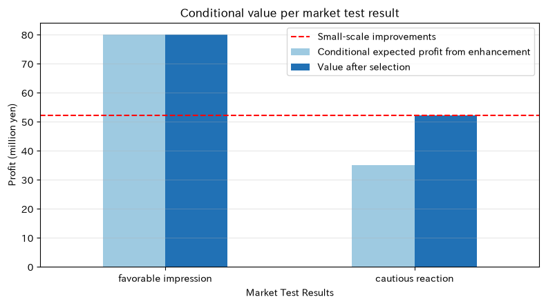
0	favorable impression	0.55	0.75	80.00	Full-scale Enhancement	80.00
1	cautious reaction	0.45	0.30	35.00	Small-scale improvements	52.00

	Expected value (million yen)
Strategy
Immediately implement the best plan.	59.75
Divergence After Market Testing	65.40

Reading the results

If the response is positive, the strategy is to switch to full-scale enhancement; if cautious, switch to small-scale improvements. Even after deducting test costs, you can change your actions based on the results, so the expected value is higher than fixing on a single proposal right away. Information alone does not create value by itself. We predefine rules for each outcome, opportunities lost during the testing period, and the impact of competitive entrants.

No.075: Bayesian Decision Making — Updating Demand Probabilities with Order Signals

Meaning in Practice

When there is an exhibition response, number of inquiries, or advance orders, overwriting the demand forecast intuitively can cause overreaction. Bayesian updates consistently integrate the original outlook with the confidence of new signals.

Approach to Analysis and Modeling

The state probability after observing signal $z$ is

$P(s\mid z)=\frac{P(z\mid s)P(s)}{\sum_{s'}P(z\mid s')P(s')}$

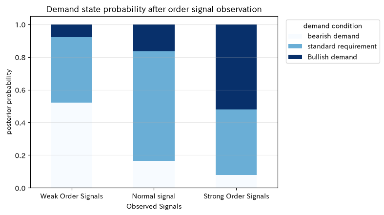
That’s right. For each signal, the posterior probability is calculated, and the action that maximizes expected profit is chosen based on that probability. The discriminative power of signals appears in likelihood $P(z\mid s)$.

Check with Python

posterior_rows = []
decision_rows = []
for signal, row in likelihood.iterrows():
    joint = row * probability
    posterior = joint / joint.sum()
    posterior_rows.append(posterior.rename(signal))
    conditional_ev = profit.mul(posterior, axis=1).sum(axis=1)
    decision_rows.append({
        "signal": signal,
        "Recommended proposal": conditional_ev.idxmax(),
        "Contingent expected profit": conditional_ev.max(),
        "Signal Occurrence Probability": joint.sum(),
    })
posterior_table = pd.DataFrame(posterior_rows)
bayes_decisions = pd.DataFrame(decision_rows).set_index("signal")
display(posterior_table)
display(bayes_decisions)

ax = posterior_table.plot(kind="bar", stacked=True, figsize=(8, 4.5), colormap="Blues")
ax.set_title("Demand state probability after order signal observation")
ax.set_xlabel("Observed Signals")
ax.set_ylabel("posterior probability")
ax.grid(axis="y", alpha=0.3)
ax.legend(title="demand condition", bbox_to_anchor=(1.02, 1), loc="upper left")
plt.xticks(rotation=0)
plt.tight_layout()
plt.show()

	bearish demand	standard requirement	Bullish demand
Weak Order Signals	0.52	0.40	0.08
Normal signal	0.17	0.67	0.17
Strong Order Signals	0.08	0.40	0.52

	Recommended proposal	Contingent expected profit	Signal Occurrence Probability
signal
Weak Order Signals	Flexibility through outsourcing	51.48	0.31
Normal signal	Facility Enhancement	68.00	0.38
Strong Order Signals	Facility Enhancement	90.16	0.31

Reading the results

A weak signal increases the probability of bearish demand, while a strong signal increases the probability of bullish demand. As a result, recommendations also change according to the signal. In practice, the likelihood is updated from past forecast accuracy and the variation in signal definitions by sales representatives is monitored. By storing post-hoc probabilities and hiring decisions, you can evaluate predictions and decisions separately afterward.

No.076: MDP — Optimizing maintenance timing based on equipment condition

Meaning in Practice

Equipment maintenance is a time trade-off between “reducing maintenance costs this term” and “preventing future breakdown costs.” Conditions are classified as normal, deteriorate, or dangerous, and the issue is treated each term as a choice between continued operation or preventive maintenance.

Approach to Analysis and Modeling

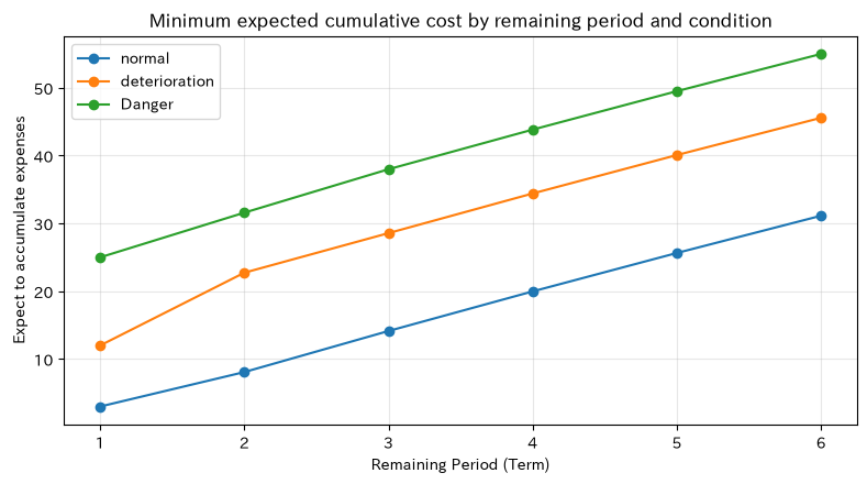
The Markov Decision Process (MDP) defines state $s$, action $a$, transition probability $P(s'\mid s,a)$, and immediate cost $c(s,a)$. The minimum expected cost for the remaining $t$ period is based on the Bellman equation.

$J_t(s)=\min_a\left[c(s,a)+\gamma\sum_{s'}P(s'\mid s,a)J_{t-1}(s')\right]$

Let’s calculate backwards. Here, we will depict six periods with a discount rate of $\gamma=0.97$.

Check with Python

machine_states = ["normal", "deterioration", "Danger"]
actions = ["Continued operation", "preventive maintenance"]
transition = {
    "Continued operation": np.array([[0.78, 0.20, 0.02], [0.08, 0.65, 0.27], [0.02, 0.18, 0.80]]),
    "preventive maintenance": np.array([[0.94, 0.06, 0.00], [0.82, 0.16, 0.02], [0.68, 0.25, 0.07]]),
}
immediate_cost = {
    "Continued operation": np.array([3, 12, 45]),
    "preventive maintenance": np.array([15, 18, 25]),
}
horizon, gamma = 6, 0.97
value = np.zeros((horizon + 1, len(machine_states)))
policy = []
for t in range(1, horizon + 1):
    q = np.column_stack([
        immediate_cost[a] + gamma * transition[a] @ value[t - 1]
        for a in actions
    ])
    value[t] = q.min(axis=1)
    policy.append([actions[i] for i in q.argmin(axis=1)])

policy_table = pd.DataFrame(
    policy, index=[f"Remaining{t}period" for t in range(1, horizon + 1)], columns=machine_states
)
display(policy_table)
display(pd.DataFrame(value[1:], index=policy_table.index, columns=machine_states).tail(1))

ax = pd.DataFrame(value[1:], columns=machine_states, index=range(1, horizon + 1)).plot(
    marker="o", figsize=(8, 4.5)
)
ax.set_title("Minimum expected cumulative cost by remaining period and condition")
ax.set_xlabel("Remaining Period (Term)")
ax.set_ylabel("Expect to accumulate expenses")
ax.grid(alpha=0.3)
plt.tight_layout()
plt.show()

	normal	deterioration	Danger
Remaining1period	Continued operation	Continued operation	preventive maintenance
Remaining2period	Continued operation	preventive maintenance	preventive maintenance
Remaining3period	Continued operation	preventive maintenance	preventive maintenance
Remaining4period	Continued operation	preventive maintenance	preventive maintenance
Remaining5period	Continued operation	preventive maintenance	preventive maintenance
Remaining6period	Continued operation	preventive maintenance	preventive maintenance

	normal	deterioration	Danger
Remaining6period	31.14	45.58	54.99

Reading the results

Under normal conditions, the basic approach is to continue operation, while in dangerous conditions, preventive maintenance is the basic approach. The assessment of deterioration depends on the remaining period and future costs, and cannot be determined solely by short-term maintenance costs. In actual production, safety, quality, and delivery impacts caused by failures are included in costs, and the probability of recovery after maintenance is estimated based on actual results. If the condition classification is too crude, different equipment behaviors may coexist within the same ‘deterioration.‘

No.077: POMDP — Managing Invisible Deterioration with Belief Probability

Meaning in Practice

In reality, it is impossible to directly observe the true state of equipment deterioration. Alarms from vibration sensors can include false alarms and missed detections, and if maintenance decisions are made solely based on the presence or absence of alarms, over-maintenance or sudden stoppages will increase.

Approach to Analysis and Modeling

In the Partial Observation Markov Decision Process (POMDP), the state of belief of deterioration $b=P(D)$ is used, not the state itself. Updates to Alert $A$

$P(D\mid A)=\frac{P(A\mid D)P(D)}{P(A\mid D)P(D)+P(A\mid H)P(H)}$

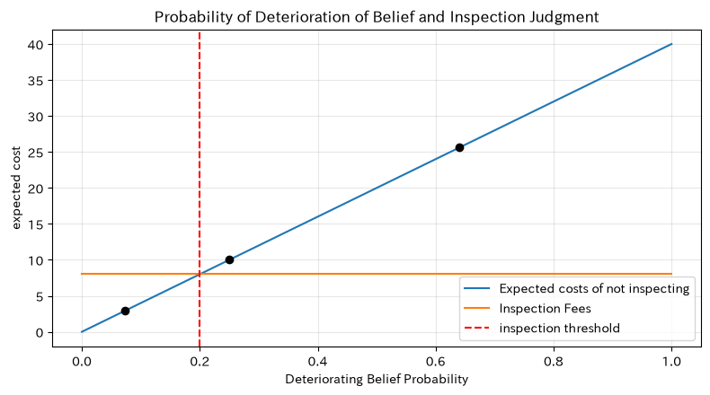
That’s right. For simplicity, we compare inspection cost 8 and expected failure cost $40b$ if not inspected, and inspect if $b>8/40=0.20$ is done.

Check with Python

prior_degraded = 0.25
p_alarm_given_degraded = 0.80
p_alarm_given_healthy = 0.15

def posterior_degraded(alarm):
    p_obs_d = p_alarm_given_degraded if alarm else 1 - p_alarm_given_degraded
    p_obs_h = p_alarm_given_healthy if alarm else 1 - p_alarm_given_healthy
    return (p_obs_d * prior_degraded) / (
        p_obs_d * prior_degraded + p_obs_h * (1 - prior_degraded)
    )

beliefs = pd.Series({
    "Before Observation": prior_degraded,
    "Alarm": posterior_degraded(True),
    "No alarm": posterior_degraded(False),
}, name="Probability of Deterioration of Belief")
pomdp_table = beliefs.to_frame()
pomdp_table["Expected costs of not inspecting"] = 40 * pomdp_table["Probability of Deterioration of Belief"]
pomdp_table["Recommended Actions"] = np.where(
    pomdp_table["Expected costs of not inspecting"] > 8, "inspect", "Continued operation"
)
display(pomdp_table)

belief_grid = np.linspace(0, 1, 101)
fig, ax = plt.subplots(figsize=(8, 4.5))
ax.plot(belief_grid, 40 * belief_grid, label="Expected costs of not inspecting")
ax.plot(belief_grid, np.full_like(belief_grid, 8), label="Inspection Fees")
ax.axvline(0.20, color="red", linestyle="--", label="inspection threshold")
ax.scatter(beliefs.values, 40 * beliefs.values, color="black", zorder=3)
ax.set_title("Probability of Deterioration of Belief and Inspection Judgment")
ax.set_xlabel("Deteriorating Belief Probability")
ax.set_ylabel("expected cost")
ax.grid(alpha=0.3)
ax.legend()
plt.tight_layout()
plt.show()

	Probability of Deterioration of Belief	Expected costs of not inspecting	Recommended Actions
Before Observation	0.25	10.00	inspect
Alarm	0.64	25.60	inspect
No alarm	0.07	2.91	Continued operation

Reading the results

With an alarm, the probability of deterioration exceeds the inspection threshold, and without an alarm, it falls below the threshold. It is important not to treat alerts as the state itself, but as ‘the probability of being updated from alarm accuracy and pre-degradation rate.’ In practice, this extends to multi-period POMDP, including continuous observations, degradation transitions, post-inspection information, and downtime. Thresholds must not be optimized to fall below safety standards, and mandatory inspections for legal and quality requirements are prioritized.

No.078: Scenario Analysis — Comparing Procurement Strategies with Compound Shocks

Meaning in Practice

When choosing suppliers, if you only look at the usual purchase price, you may overlook supply losses caused by material costs, yen depreciation, and logistics disruptions. Scenario analysis creates multiple coherent external environments and visualizes the weaknesses of each strategy.

Approach to Analysis and Modeling

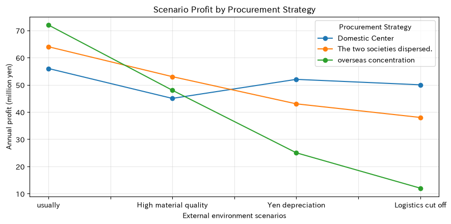
A scenario is not a fluctuation of the predicted value, but a set of causally consistent variables. Here, we compare domestic concentration, two-company dispersion, and overseas concentration in terms of profits from material costs, yen depreciation, and logistics disruptions. In addition to probability-weighted values, it also shows worst-case profits and maximum regrets. If the reliability of scenario probabilities is low, prioritize ranking stability over expected values.

Check with Python

sourcing_profit = pd.DataFrame(
    [[56, 45, 52, 50], [64, 53, 43, 38], [72, 48, 25, 12]],
    index=["Domestic Center", "The two societies dispersed.", "overseas concentration"],
    columns=["usually", "High material quality", "Yen depreciation", "Logistics cut off"],
)
scenario_prob = pd.Series([0.45, 0.20, 0.20, 0.15], index=sourcing_profit.columns)
scenario_summary = pd.DataFrame({
    "Probability Increases Profit": sourcing_profit.mul(scenario_prob, axis=1).sum(axis=1),
    "worst profit": sourcing_profit.min(axis=1),
    "Maximum Regret": (sourcing_profit.max(axis=0) - sourcing_profit).max(axis=1),
})
display(sourcing_profit)
display(scenario_summary)

ax = sourcing_profit.T.plot(marker="o", figsize=(9, 4.5))
ax.set_title("Scenario Profit by Procurement Strategy")
ax.set_xlabel("External environment scenarios")
ax.set_ylabel("Annual profit (million yen)")
ax.grid(alpha=0.3)
ax.legend(title="Procurement Strategy")
plt.tight_layout()
plt.show()

	usually	High material quality	Yen depreciation	Logistics cut off
Domestic Center	56	45	52	50
The two societies dispersed.	64	53	43	38
overseas concentration	72	48	25	12

	Probability Increases Profit	worst profit	Maximum Regret
Domestic Center	52.10	45	16
The two societies dispersed.	53.70	38	12
overseas concentration	48.80	12	38

Reading the results

Overseas concentration usually brings maximum profits, but the weak yen and disruptions in logistics can cause significant declines. Domestically-centered companies have smaller upside but higher worst-case profits, and diversification between two companies is intermediate. The adoption plan is not determined solely by probability-weighted profit; constraints include the loss caused by supply stoppages to the customer line, the time required for substitution certification, and the minimum supply amount on the BCP.

No.079: Sensitivity Analysis — Understanding the Boundary of Bullish Demand Probability Switching

Meaning in Practice

The probabilities in decision tables are not fixed truths. If the sales department changes the conclusion simply by raising the probability of bullish demand from 25% to 20%, then that investment proposal is sensitive to assumptions. Sensitivity analysis indicates the boundaries where re-approval is necessary.

Approach to Analysis and Modeling

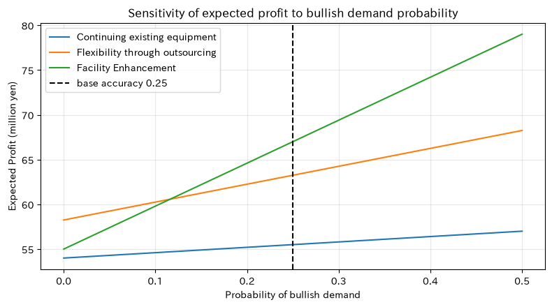
Fix the bearish demand probability at 0.25 and move the bullish demand probability $p_H$ between 0 and 0.50. The standard demand probability is $0.75-p_H$. The expected profit of each option is a linear function of $p_H$, and the point where the lines of the two options intersect is the boundary of the choice switch. If multiple parameters are uncertain, it is extended to two-dimensional sensitivity analysis or probabilistic sensitivity analysis.

Check with Python

p_high_grid = np.linspace(0, 0.50, 101)
sensitivity = pd.DataFrame(index=p_high_grid)
for plan in plans:
    sensitivity[plan] = (
        0.25 * profit.loc[plan, "bearish demand"]
        + (0.75 - p_high_grid) * profit.loc[plan, "standard requirement"]
        + p_high_grid * profit.loc[plan, "Bullish demand"]
    )
sensitivity.index.name = "Bullish demand probability"
sensitivity["Recommended proposal"] = sensitivity.idxmax(axis=1)
switches = sensitivity["Recommended proposal"].ne(sensitivity["Recommended proposal"].shift())
display(sensitivity.loc[switches, [*plans, "Recommended proposal"]])

fig, ax = plt.subplots(figsize=(8, 4.5))
for plan in plans:
    ax.plot(sensitivity.index, sensitivity[plan], label=plan)
ax.axvline(0.25, color="black", linestyle="--", label="base accuracy 0.25")
ax.set_title("Sensitivity of expected profit to bullish demand probability")
ax.set_xlabel("Probability of bullish demand")
ax.set_ylabel("Expected Profit (million yen)")
ax.grid(alpha=0.3)
ax.legend()
plt.tight_layout()
plt.show()

	Continuing existing equipment	Flexibility through outsourcing	Facility Enhancement	Recommended proposal
Bullish demand probability
0.00	54.00	58.25	55.00	Flexibility through outsourcing
0.12	54.72	60.65	60.76	Facility Enhancement

Reading the results

In areas with low probability of bullish demand, flexible outsourcing proposals are advantageous; when prices rise, facility expansion plans are advantageous, and the transition boundaries can be checked from the table. If the baseline value of 25% is sufficiently far from the boundary, a small forecast correction will not change the conclusion. If close to the boundary, options like phased investments, contracts that can be terminated, or additional investigations are valuable.

No.080: Robust Optimization — Creating Production Allocations That Withstand Reduced Machining Time

Meaning in Practice

Optimizing the product mix only in nominal standard time results in plans becoming unexecutable on days when machining times worsen due to tool wear or operator differences. Robust optimization requires a plan that enforces constraints in all cases of a predefined set of uncertainties.

Approach to Analysis and Modeling

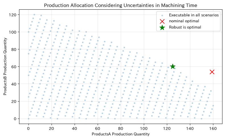
Let the quantity of products A and B be $x_A,x_B$, $8,11$ marginal profit, and the available time be 480 minutes. For the processing time scenario set $\mathcal U$,

$\max_{x_A,x_B}\ 8x_A+11x_B$

$t_A^{(u)}x_A+t_B^{(u)}x_B\le480\quad(\forall u\in\mathcal U)$

It meets the requirements. To protect all cases, we are conservative, but you can also reduce plans changes, overtime, and delivery delays. Here, we will list all integer lattices.

Check with Python

time_scenarios = pd.DataFrame(
    [[2.0, 3.0], [2.4, 3.0], [2.0, 3.8]],
    index=["pretext", "ProductsAProcessing deterioration", "ProductsBProcessing deterioration"],
    columns=["ProductsA", "ProductsB"],
)
candidates = pd.DataFrame(
    [(a, b) for a in range(161) for b in range(121)],
    columns=["ProductsA", "ProductsB"],
)
candidates["marginal interest"] = 8 * candidates["ProductsA"] + 11 * candidates["ProductsB"]
for scenario, times in time_scenarios.iterrows():
    candidates[f"usage_time_{scenario}"] = candidates[["ProductsA", "ProductsB"]] @ times

nominal_feasible = candidates["usage_time_pretext"] <= 480
robust_feasible = candidates[[f"usage_time_{s}" for s in time_scenarios.index]].max(axis=1) <= 480
nominal_best = candidates.loc[candidates.loc[nominal_feasible, "marginal interest"].idxmax()]
robust_best = candidates.loc[candidates.loc[robust_feasible, "marginal interest"].idxmax()]
comparison = pd.DataFrame([nominal_best, robust_best], index=["nominal optimal", "Robust is optimal"])
display(time_scenarios)
display(comparison[["ProductsA", "ProductsB", "marginal interest", *[f"usage_time_{s}" for s in time_scenarios.index]]])

fig, ax = plt.subplots(figsize=(8, 5))
sample = candidates.iloc[::25]
ax.scatter(sample.loc[robust_feasible.iloc[::25], "ProductsA"],
           sample.loc[robust_feasible.iloc[::25], "ProductsB"],
           s=8, alpha=0.25, label="Executable in all scenarios")
ax.scatter(nominal_best["ProductsA"], nominal_best["ProductsB"], marker="x", s=120,
           color="red", label="nominal optimal")
ax.scatter(robust_best["ProductsA"], robust_best["ProductsB"], marker="*", s=180,
           color="green", label="Robust is optimal")
ax.set_title("Production Allocation Considering Uncertainties in Machining Time")
ax.set_xlabel("ProductsA Production Quantity")
ax.set_ylabel("ProductsB Production Quantity")
ax.grid(alpha=0.3)
ax.legend()
plt.tight_layout()
plt.show()

	ProductsA	ProductsB
pretext	2.00	3.00
ProductsAProcessing deterioration	2.40	3.00
ProductsBProcessing deterioration	2.00	3.80

	ProductsA	ProductsB	marginal interest	usage_time_pretext	usage_time_ProductsAProcessing deterioration	usage_time_ProductsBProcessing deterioration
nominal optimal	159.00	54.00	1,866.00	480.00	543.60	523.20
Robust is optimal	125.00	60.00	1,660.00	430.00	480.00	478.00

Reading the results

Nominal optimization offers high profits, but if the processing time for product B worsens, it exceeds 480 minutes. Robust optimization gives up some marginal profit and selects an allocation that is feasible for all scenarios. This difference is the “robustness insurance premium.” If the uncertainty set is overly broadened, the plan becomes conservative, so the scope is regularly updated based on past performance, facility conditions, and areas for improvement, and compared to probability constraints that allow for excess probabilities.

Practical Implications Seen Through Target Exercise

1. Separating expected value from downside risk: Proposals with the highest average profit may not align with those that can withstand bad years.
2. Clearly define value standards: Use utility and allowable loss to transform “careful judgment” into reproducible rules.
3. Decide on actions after information is obtained: Market testing and sensor implementation are valuable when observations change decision-making.
4. Probability updates: Bayesian updates allow you to consistently integrate forward forecasts and new information, keeping a history of decisions.
5. Handling time and state: MDP evaluates not only current costs but also the impact of actions on future conditions.
6. Have a probability of being in an invisible state: The POMDP belief state allows you to factor in false alarms and missed alerts in your decisions.
7. Sharing the boundaries of assumptions: Scenario analysis and sensitivity analysis make the conditions under which conclusions change a common language across departments.
8. Ensuring Feasibility: Robust optimization quantifies the trade-off between nominal profit and the risk of plan changes.

What is necessary for practical implementation

1. Create a decision ledger

Record who made what decisions, when, and what was made, and how choices, status, evaluation periods, KPIs, and constraints were set. Don’t confuse prediction accuracy with decision-making quality, so you can later evaluate whether the information at the time was valid.

2. Manage the basis for probabilities and losses

Demand probability, failure transitions, alarm accuracy, and downtime losses are linked to data periods and estimation methods. If the number of cases is small, do not overestimate the points and leave the range of expert judgment and credit ranges to consider. Mandatory conditions regarding safety, laws, and quality are not exchanged for profit.

3. Agree on multiple KPIs and approval boundaries

Expected profit, CVaR, supply compliance rate, maximum downtime, etc., are listed together, and a decision is made to determine which levels are below which the proposal should be rejected or reconsidered. Utility coefficients and scenario probabilities are not numbers meant to hide management decisions, but rather as assumptions used to explain those decisions.

4. Shift from small-scale decision-making to closed-loop

Within a single group of equipment or products, we → ‘predict proposals→ approve→ execute→ and → results probabilities update.’ After confirming the adoption or rejection of model proposals and reasons and confirming reproducibility, integration with ERP, MES, and equipment data and the scope of automation are expanded.

5. Design Model Monitoring and Exception Procedures

Monitor probability correction, prediction errors, state transitions, constraint violations, and manual interventions. For areas outside the learning scope, such as disasters, new products, or equipment modifications, automatic decisions are stopped, and responsibilities are defined so that people can switch to alternative procedures.

Conclusion

From No.071 to No.080, we covered from expected profits, downside risk and utility, stepwise decision-making, Bayesian updates, temporal changes in equipment condition, partial observations, composite scenarios, assumption sensitivity, and robust production allocation.

In manufacturing decision-making, simply improving forecasting accuracy does not eliminate uncertainty. The key is to clearly state what is uncertain, which losses to avoid, how to change actions when information is received, and to what extent the plan will be followed. By recording assumptions and achievements in small decisions and continuously updating probabilities, losses, and constraints, analysis can move from meeting materials to actionable decision-making platforms.

Consultations for Corporations

At Suri Kobo, we offer consultations for decision-making under uncertainty in manufacturing, demand and failure risk assessment, simulation, mathematical optimization, and the planning of decision-making infrastructure, as well as support for implementation and in-house production.

• Quantitative comparison of capital investment, outsourcing, inventory, and procurement strategies
• Management decision support using expected values, CVaR, scenarios, and sensitivity analysis
• MDP/POMDP models for equipment maintenance, Bayesian updates using sensor information
• Robust optimization considering uncertainties in demand and processing time
• Designing a decision-making platform that connects ERP, MES, and equipment data
• Corporate training covering Python, statistics, simulation, and optimization

📩 Contact Us: surikobo.co.jp/contact
Please feel free to consult us first.