100 Exercises / Probability Statistics / 100 Exercise Points in Probability & Statistical Marketing Applications

Learning Manufacturing Simulation with Python | 10 Exercises from Monte Carlo to Digital Twins

2020-06-02

Factory Management That Anticipates Fluctuations: 10 Exercise-Down Simulations for Industrial Pump Factories

This article uses a fictional industrial pump factory as the subject and addresses ten Monte Carlo, discrete events, agent base, queues, system dynamics, inventory, production lines, supply chain, demand, digital twin themes as a continuous decision-making process.

The goal is not to implement the method itself, but to enable replicable virtual experiments to explain “how far profit plans can be downstream,” “where to allocate equipment, personnel, and inventory,” and “how to prepare for supply disruptions and demand fluctuations.” The published data is generated in Python and does not depend on external data.

[!NOTE] This material is a notebook previously used by Surikoubo (or personally by the representative, Kazuyama), and has been reconstructed, edited, and published with the company’s permission.
All data listed is fictional and has no relation whatsoever to real companies, factories, or figures.

Introduction: Practical Challenges in Manufacturing Covered in This Article

The target factory processes, assembles, and inspects standard and high-pressure industrial pumps before shipping them to corporate customers. Demand, processing time, equipment failures, and material delivery times fluctuate daily. Production managers must simultaneously assess not only monthly plans but also daily work-in-progress, material inventory, support personnel, express transportation, and delivery deadline responses to customers.

Simulation is not a tool for predicting the future in a single point. It is a “virtual experiment” that models reality within the scope necessary for decision-making and safely compares measures that have not yet been implemented. In this article, in addition to averages, we gradually incorporate distribution, time sequence, interactions, and feedback into the model.

Common situations on site

Although the annual profit is planned to be profitable, the downside cannot be explained by the overlapping of declining demand, material costs, and shutdowns.
You know the average operating rate of each piece of equipment, but you don’t know where or how many minutes the rig will wait.
Maintenance staff, workers, transport vehicles, and suppliers make local judgments, making the impact on overall KPIs unclear.
Safety stock was uniformly increased, resulting in fewer out-of-stock stocks but higher inventory values and disposal
The assumptions for demand forecasting, production planning, and procurement planning differ by department.
Digital twins have been introduced, but there is no operational model update based on on-site experience.

A common challenge is Pushing fluctuations and temporal dependencies into average values.

Why is this issue so difficult to judge?

The manufacturing system is nonlinearity. When the operating rate approaches 100%, waiting times increase sharply, and a single missing component can trigger stoppages in subsequent processes. Increasing order volumes reduces stockouts, but increases inventory costs and the risk of obsolescence. Moreover, the main actors on the ground do not share the same information and act according to different rules.

Therefore, average profit or average lead time alone is not enough. This article also lists profit downward quintiles, on-time delivery rate, waiting time, work-in-progress inventory, fulfillment rate, backlog, recovery time, and more, while simultaneously evaluating Expected value, risk, response speed, cost.

Overview of Exercise covered this time

No.	Theme	Main Questions	Main Outputs
081	Monte Carlo	How far can profits decline?	Profit Distribution, Deficit Probability
082	discrete event	When jobs are shipped and where to wait	Event Logs, Lead Time
083	Agent-based	How individual conservation decisions affect the entire population	Downtime rate, preventive maintenance rate
084	queue	How many inspectors should be assigned?	Wait times and service levels
085	System Dynamics	How do orders, capacity, and backlog circulate?	Trends in Inventory and Order Backlog
086	Inventory Simulation	How to choose ordering policies	Fill Rate, Inventory Costs
087	Production Line Simulation	Which process should we direct our improvement investments to?	Throughput and process utilization rate
088	Supply Chain Simulation	How to prepare for supply interruptions	Out-of-stock, total cost, recovery time
089	Demand Simulation	How to compare capability proposals in S&OP	Monthly Distribution and Excess Probability
090	Digital twin	How to update models based on achievements	Status updates, scenario comparison

Preparing the Python environment

NumPy is used for random numbers and numerical calculations, pandas for representing events and KPIs, and matplotlib for visualization. The random number generator is fixed as a default_rng(SEED + Number) for each purpose, ensuring that rerunning the code yields the same result. All graphs are created using matplotlib.

import heapq
import platform

import japanize_matplotlib
import matplotlib.pyplot as plt
import numpy as np
import pandas as pd
from IPython.display import display

SEED = 42
pd.set_option("display.max_columns", 20)
pd.set_option("display.float_format", lambda x: f"{x:,.2f}")

print(f"Python: {platform.python_version()}")
print(f"NumPy: {np.__version__} / pandas: {pd.__version__}")
print(f"random numberseed: {SEED}")

Python: 3.13.1
NumPy: 2.5.1 / pandas: 3.0.3
Random seed: 42

Creation of Fictional Data

We assume two products: the standard P-100 and the high-pressure P-200. We prepare a common master for costs, pricing, demand, standard times for the three main processes, and daily capacity. In individual exercises, failures, demand, and delivery schedule fluctuations are applied based on this master.

In practice, you first define whether standard time is net time or margin, whether demand is on the order date or preferred delivery date, and whether out-of-stock results in backlog or lost order. Before the accuracy of the simulation, discrepancies in the meaning of the data can change the conclusion.

products = pd.DataFrame({
    "Products": ["P-100 Standard model", "P-200 High Pressure Resistance Type"],
    "average_monthly_demand_platform": [620, 310],
    "sale_price_ten_thousand_yen": [18.0, 27.0],
    "material_cost_ten_thousand_yen": [8.2, 12.5],
    "processing_minutes": [18, 26],
    "assembly_minutes": [22, 34],
    "inspection_minutes": [14, 24],
}).set_index("Products")

resources = pd.DataFrame({
    "Project": ["processing", "assembly", "inspection"],
    "Facilities and Number of Personnel": [2, 3, 2],
    "net_daily_time_minutes": [450, 450, 450],
    "coefficient_of_variation": [0.18, 0.12, 0.22],
}).set_index("Project")

print("Product Master")
display(products)
print("Process Capability Master")
display(resources)

Product Master

	average_monthly_demand_platform	sale_price_ten_thousand_yen	material_cost_ten_thousand_yen	processing_minutes	assembly_minutes	inspection_minutes
Products
P-100 Standard model	620	18.00	8.20	18	22	14
P-200 High Pressure Resistance Type	310	27.00	12.50	26	34	24

Process Capability Master

	Facilities and Number of Personnel	net_daily_time_minutes	coefficient_of_variation
Project
processing	2	450	0.18
assembly	3	450	0.12
inspection	2	450	0.22

No.081: Monte Carlo — Measuring the Downside of Annual Profits by Probability

Meaning in Practice

If you set the budget’s sales, material unit price, and downtime into one point, the planned profit is determined as one. However, in management decisions, not only average profit but also loss amounts in certain cases and probability of losses are necessary. This directly leads to consideration of capital investment quotas, working capital, and long-term contract prices.

Approach to Analysis and Modeling

Annual profit for scenario $s$

$\Pi_s=Q_s(P-C_{m,s}-C_v)-F-C_{d,s}$

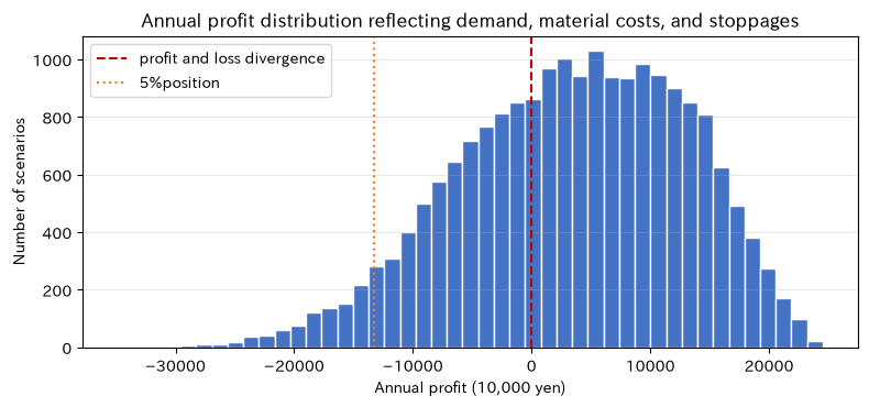
Let’s say so. $Q$ is sales volume, $P$ is price, $C_m$ is material cost, $C_v$ is variable processing cost, $F$ is fixed cost, $C_d$ is stopping loss. Input variables are repeatedly generated from probability distributions, and $P(\Pi<0)$ and 5% quantiles (profits exceeding 95% of cases) are evaluated.

Check with Python

mc_rng = np.random.default_rng(SEED + 81)
n_mc = 20_000
annual_demand = np.maximum(0, mc_rng.normal(11_200, 1_250, n_mc))
material_cost = mc_rng.triangular(9.2, 10.0, 12.4, n_mc)  # 10,000 yen per vehicle
downtime_days = mc_rng.poisson(8, n_mc)
selling_price = 21.2
variable_cost = 3.6
fixed_cost = 73_000
capacity = 11_800
sales = np.minimum(annual_demand, capacity - downtime_days * 28)
profit = sales * (selling_price - material_cost - variable_cost) - fixed_cost - downtime_days * 55

profit_kpi = pd.Series({
    "average_profit_ten_thousand_yen": profit.mean(),
    "interest5%position_ten_thousand_yen": np.quantile(profit, 0.05),
    "interest95%position_ten_thousand_yen": np.quantile(profit, 0.95),
    "deficit probability": (profit < 0).mean(),
}, name="value")
display(profit_kpi.to_frame())

fig, ax = plt.subplots(figsize=(8, 3.8))
ax.hist(profit, bins=45, color="#4472C4", edgecolor="white")
ax.axvline(0, color="#C00000", linestyle="--", label="profit and loss divergence")
ax.axvline(np.quantile(profit, 0.05), color="#ED7D31", linestyle=":", label="5%position")
ax.set_title("Annual profit distribution reflecting demand, material costs, and stoppages")
ax.set_xlabel("Annual profit (10,000 yen)")
ax.set_ylabel("Number of scenarios")
ax.grid(axis="y", alpha=0.3)
ax.legend()
plt.tight_layout()
plt.show()

	value
average_profit_ten_thousand_yen	3,384.79
interest5%position_ten_thousand_yen	-13,233.85
interest95%position_ten_thousand_yen	17,770.93
deficit probability	0.36

png

Reading the results

Even if the average profit is positive, if the distribution is to the left of zero, the risk of losses remains. The 5% percentile is a conservative standard for discussing financial capacity and investment limits. However, the shape of the distribution depends on the input assumption. In practice, we estimate the correlation between demand and material prices, the time lag for price pass-through, and the capability ceiling based on actual results, and also check the conditions for entering deficit scenarios.

No.082: Discrete Event — Recreating Process Competition and Job Waiting

Meaning in Practice

After machining is complete, the product proceeds to assembly and waits until equipment becomes available. In systems where the state changes at the point of events such as “arrival” or “processing complete,” discrete event simulation is more efficient than simply tracking the time. It can be used for responding to deadlines, reducing work-in-progress, and considering the order of preparation.

Approach to Analysis and Modeling

The start and completion times of process $k$ of Job $j$

$S_{j,k}=\max(A_{j,k},R_k),\qquad C_{j,k}=S_{j,k}+P_{j,k}$

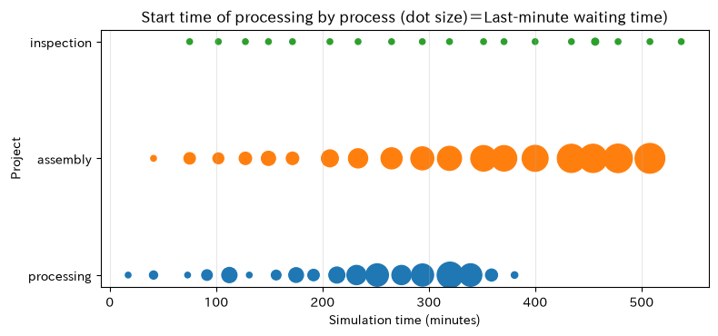
Let’s say so. $A$ is the arrival of the process, $R$ is the time when resources become available, and $P$ is the processing time. Events are processed in priority queues arranged by time, and wait times and lead times are aggregated from the event log.

Check with Python

des_rng = np.random.default_rng(SEED + 82)
routes = ["processing", "assembly", "inspection"]
resource_ready = {m: 0.0 for m in routes}
event_queue = []
log = []
n_jobs = 18
arrival_times = np.cumsum(des_rng.exponential(16, n_jobs))

for j, arrival in enumerate(arrival_times):
    heapq.heappush(event_queue, (arrival, j, 0))

while event_queue:
    arrival, job, step = heapq.heappop(event_queue)
    machine = routes[step]
    means = [20, 27, 18]
    duration = des_rng.lognormal(np.log(means[step]), 0.18)
    start = max(arrival, resource_ready[machine])
    finish = start + duration
    resource_ready[machine] = finish
    log.append([job, machine, step + 1, arrival, start, finish, start - arrival])
    if step + 1 < len(routes):
        heapq.heappush(event_queue, (finish, job, step + 1))

event_log = pd.DataFrame(log, columns=["job", "Project", "Smooth engineering", "Arrival", "start", "completed", "waiting time"])
job_kpi = event_log.groupby("job").agg(invest=("Arrival", "min"), completed=("completed", "max"), mass_waiting=("waiting time", "sum"))
job_kpi["lead time"] = job_kpi["completed"] - job_kpi["invest"]
display(event_log.head(10))
display(job_kpi.describe().loc[["mean", "50%", "max"]])

fig, ax = plt.subplots(figsize=(8, 3.8))
for i, machine in enumerate(routes):
    part = event_log[event_log["Project"] == machine]
    ax.scatter(part["start"], [i] * len(part), s=part["waiting time"] * 5 + 20, label=machine)
ax.set_yticks(range(len(routes)), routes)
ax.set_title("Start time of processing by process (dot size)＝Last-minute waiting time)")
ax.set_xlabel("Simulation time (minutes)")
ax.set_ylabel("Project")
ax.grid(axis="x", alpha=0.3)
plt.tight_layout()
plt.show()

	job	Project	Smooth engineering	Arrival	start	completed	waiting time
0	0	processing	1	17.26	17.26	41.15	0.00
1	1	processing	1	36.88	41.15	62.93	4.27
2	0	assembly	2	41.15	41.15	75.09	0.00
3	1	assembly	2	62.93	75.09	102.12	12.16
4	2	processing	1	73.18	73.18	91.40	0.00
5	0	inspection	3	75.09	75.09	93.83	0.00
6	3	processing	1	81.55	91.40	112.45	9.85
7	4	processing	1	87.67	112.45	128.27	24.78
8	2	assembly	2	91.40	102.12	127.52	10.72
9	1	inspection	3	102.12	102.12	117.42	0.00

	invest	completed	mass_waiting	lead time
mean	177.21	322.24	79.07	145.04
50%	182.37	325.33	77.44	144.69
max	379.36	555.73	176.19	233.52

png

Reading the results

Even within the same standard time, lead times for each job vary depending on the overlapping arrivals. Processes or times with large points are places where waiting has accumulated. We look not only at the average waiting time but also at the maximum value and job breakdown to create candidates for increases, priority orders, and lot splits. The production model adds events such as multiple equipment breakdowns, scheduling, breaks, and adjustments.

No.083: Agent-Based — Capturing Local Decisions and Equipment Behavior by Security Personnel

Meaning in Practice

The condition of deterioration varies by equipment, and the maintenance staff patrol for limited time. The interaction where each facility issues alerts and the maintenance team determines priorities is a problem that is difficult to express with aggregation alone. It can be used to design preventive maintenance rules, patrol capabilities, and alarm thresholds.

Approach to Analysis and Modeling

Each piece of equipment is designated as an agent with a status $h_i(t)\in[0,1]$ , and each quarter $d_i(t)$ deterioration and recovery $r_i(t)$ through maintenance.

$h_i(t+1)=\min\{1,\max[0,h_i(t)-d_i(t)+r_i(t)]\}$

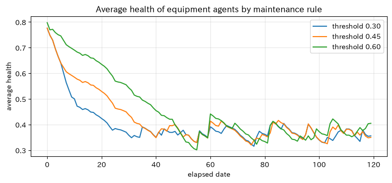
will be updated. Maintenance agents treat up to two devices per day that fall below the threshold, ranked by health level. Adjust thresholds to compare the trade-off between stopping failures and the number of maintenance cycles.

Check with Python

def run_agents(threshold, seed, days=120, n_machines=18):
    agent_rng = np.random.default_rng(seed)
    health = agent_rng.uniform(0.65, 1.0, n_machines)
    failures = maintenance = lost_hours = 0
    history = []
    for day in range(days):
        health -= agent_rng.gamma(shape=2.0, scale=0.015, size=n_machines)
        failed = health <= 0.12
        failures += failed.sum()
        lost_hours += failed.sum() * 7.5
        health[failed] = 0.58  # Post-event repair
        targets = np.where((health < threshold) & (~failed))[0]
        targets = targets[np.argsort(health[targets])][:1]
        maintenance += len(targets)
        lost_hours += len(targets) * 1.2
        health[targets] = np.minimum(1.0, health[targets] + 0.38)
        history.append([day, health.mean(), failures, maintenance])
    return failures, maintenance, lost_hours, pd.DataFrame(history, columns=["days", "average health", "cumulative fault", "Cumulative preventive maintenance"])

agent_rows = []
histories = {}
for threshold in [0.30, 0.45, 0.60]:
    # Comparing only the conservation rules with the same degraded random number (common random number method)
    f, m, lost, hist = run_agents(threshold, SEED + 83)
    agent_rows.append([threshold, f, m, lost])
    histories[threshold] = hist
agent_result = pd.DataFrame(agent_rows, columns=["Conservation threshold", "Number of Failures", "Number of preventive maintenance cases", "Stop conversion time"])
display(agent_result)

fig, ax = plt.subplots(figsize=(8, 3.8))
for threshold, hist in histories.items():
    ax.plot(hist["days"], hist["average health"], label=f"threshold {threshold:.2f}")
ax.set_title("Average health of equipment agents by maintenance rule")
ax.set_xlabel("elapsed date")
ax.set_ylabel("average health")
ax.grid(alpha=0.3)
ax.legend()
plt.tight_layout()
plt.show()

	Conservation threshold	Number of Failures	Number of preventive maintenance cases	Stop conversion time
0	0.30	32	109	370.80
1	0.45	28	114	346.80
2	0.60	26	119	337.80

png

Reading the results

A high threshold increases early preventive maintenance, suppressing failures while increasing planned downtime. Evaluations are conducted not only by the number of failures but also by the equivalent downtime time and maintenance costs. Since results fluctuate probabilistically, each rule is traditionally iterated across multiple seeds. In practice, equipment importance, parts inventory, security staff’s skills, and priority rules for simultaneous failures are also considered agent attributes.

No.084: Queue — Determining the Number of Final Inspection Personnel Based on Service Level

Meaning in Practice

If products arrive irregularly in the inspection process, waiting occurs even if the average processing capacity exceeds the average arrival volume. Increasing the number of inspectors reduces waiting times, but increases labor costs. By using the inspection completion rate until the shipping deadline, you can compare personnel proposals based on delivery service levels.

Approach to Analysis and Modeling

If we set the arrival rate as $\lambda$ , the processing rate per person as $\mu$ , and the number of counters as $c$ , then the usage rate is

$\rho=\frac{\lambda}{c\mu}$

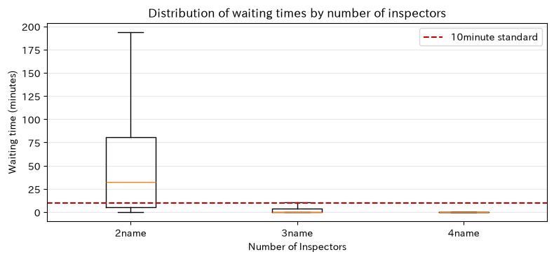
That’s right. $\rho\ge1$ the queue will be long-term and dissipate. Here, we simulate the M/M/c ratio assuming arrival and processing of the exponential distribution, and compare the average wait rate with the rate of “testing starts within 10 minutes.”

Check with Python

def simulate_queue(servers, seed, n=3000, arrival_rate=5.2, service_rate=3.0):
    queue_rng = np.random.default_rng(seed)
    arrivals = np.cumsum(queue_rng.exponential(60 / arrival_rate, n))
    service = queue_rng.exponential(60 / service_rate, n)
    ready = np.zeros(servers)
    waits = np.zeros(n)
    for i, (arrival, duration) in enumerate(zip(arrivals, service)):
        k = np.argmin(ready)
        start = max(arrival, ready[k])
        waits[i] = start - arrival
        ready[k] = start + duration
    return waits

queue_rows = []
queue_samples = {}
for c in [2, 3, 4]:
    waits = simulate_queue(c, SEED + 840 + c)
    queue_samples[c] = waits
    queue_rows.append([c, 5.2 / (c * 3.0), waits.mean(), np.quantile(waits, 0.95), (waits <= 10).mean()])
queue_result = pd.DataFrame(queue_rows, columns=["Number of Inspectors", "utilization rate", "average_waiting_time_minutes", "wait95%quantile", "10Start rate within minutes"])
display(queue_result)

fig, ax = plt.subplots(figsize=(8, 3.8))
ax.boxplot([queue_samples[c] for c in [2, 3, 4]], tick_labels=["2name", "3name", "4name"], showfliers=False)
ax.axhline(10, color="#C00000", linestyle="--", label="10minute standard")
ax.set_title("Distribution of waiting times by number of inspectors")
ax.set_xlabel("Number of Inspectors")
ax.set_ylabel("Waiting time (minutes)")
ax.grid(axis="y", alpha=0.3)
ax.legend()
plt.tight_layout()
plt.show()

	Number of Inspectors	utilization rate	average_waiting_time_minutes	wait95%position_minutes	10Start rate within minutes
0	2	0.87	48.88	156.23	0.31
1	3	0.58	5.24	29.70	0.82
2	4	0.43	1.08	8.09	0.97

png

Reading the results

For proposals with high usage rates, the upper end of the waiting time will be significantly longer. Instead of just looking at average wait times, we link the start rate to the 95% or within 10 minutes to the shipping deadline. If the improvement in the four-person proposal is small, support during busy hours rather than constant staff increases is a good option. If the arrival is in lots and processing times are by product, the actual distribution is directly resampled.

No.085: System Dynamics — Viewing Backlog and Ability Adjustment Feedback

Meaning in Practice

As orders increase, the backlog builds up, and overtime and support work boost shipping capacity. However, capacity adjustment is delayed, and if you increase it too much, inventory can balloon, which can lead to a reduction in the process. It can be used to align the timelines for S&OP, workforce planning, and production increase decisions.

Approach to Analysis and Modeling

Inventory $I_t$ and $B_t$ backorders are stocked, production and shipping are the flow, and daily difference equations are used.

$I_{t+1}=I_t+P_t-S_t,\qquad B_{t+1}=B_t+D_t-S_t$

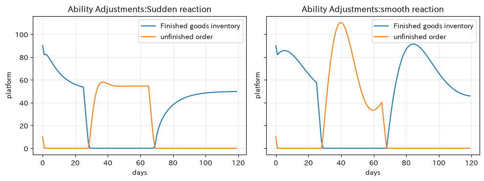
I will update you. Ability $C_t$ reacts to the difference from the target backlog but moves later due to the adjustment coefficient. Compare sudden and smooth responses.

Check with Python

def system_dynamics(adjustment, days=120):
    demand = np.full(days, 42.0)
    demand[25:65] = 58.0
    inventory = np.zeros(days)
    backlog = np.zeros(days)
    capacity = np.zeros(days)
    shipment = np.zeros(days)
    inventory[0], backlog[0], capacity[0] = 90, 10, 44
    for t in range(days - 1):
        production = capacity[t]
        shipment[t] = min(inventory[t] + production, demand[t] + backlog[t])
        inventory[t + 1] = max(0, inventory[t] + production - shipment[t])
        backlog[t + 1] = max(0, backlog[t] + demand[t] - shipment[t])
        target_capacity = 44 + 0.22 * (backlog[t] - 20) - 0.08 * (inventory[t] - 80)
        capacity[t + 1] = np.clip(capacity[t] + adjustment * (target_capacity - capacity[t]), 30, 70)
    return pd.DataFrame({"days": np.arange(days), "need": demand, "Inventory": inventory, "unfinished order": backlog, "ability": capacity})

fast_sd = system_dynamics(0.55)
smooth_sd = system_dynamics(0.12)
sd_kpi = pd.DataFrame({
    "adjustment policy": ["Sudden reaction", "smooth reaction"],
    "Maximum Order Backlog": [fast_sd["unfinished order"].max(), smooth_sd["unfinished order"].max()],
    "Maximum inventory": [fast_sd["Inventory"].max(), smooth_sd["Inventory"].max()],
    "Maximum daily capacity changes": [fast_sd["ability"].diff().abs().max(), smooth_sd["ability"].diff().abs().max()],
})
display(sd_kpi)

fig, axes = plt.subplots(1, 2, figsize=(10, 3.8), sharey=True)
for ax, df, title in zip(axes, [fast_sd, smooth_sd], ["Sudden reaction", "smooth reaction"]):
    ax.plot(df["days"], df["Inventory"], label="Finished goods inventory")
    ax.plot(df["days"], df["unfinished order"], label="unfinished order")
    ax.set_title(f"Ability Adjustments:{title}")
    ax.set_xlabel("days")
    ax.set_ylabel("platform")
    ax.grid(alpha=0.3)
    ax.legend()
plt.tight_layout()
plt.show()

	adjustment policy	Maximum Order Backlog	Maximum inventory	Maximum daily capacity changes
0	Sudden reaction	58.05	90.00	2.97
1	smooth reaction	110.36	91.40	1.86

png

Reading the results

Rapid responses can help reduce order backlogs quickly, but the policy is to increase capacity changes and inventory fluctuations. Smooth responses stabilize operations but increase customer wait times during surges in demand. Which one you choose depends on the cost of delivery delays, overtime or support change costs, and inventory costs. In practice, delays in recruitment, training, and equipment procurement are explicitly included.

No.086: Inventory Simulation — Comparing Order Points and Order Quantities by Cost and Fulfillment Rate

Meaning in Practice

Shortages of key seal parts halt the line, but excess inventory locks in funds and increases waste during design changes. In an environment where demand and procurement lead times fluctuate, it is necessary not only to calculate averages but also to reproduce ordering policies as daily operations.

Approach to Analysis and Modeling

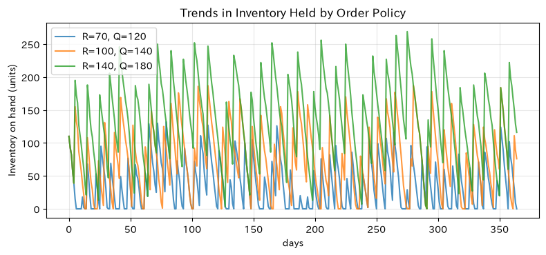
Evaluate the $(Q,R)$ policy of placing $IP=$ inventory positions as inventory + backlog - backlog, and ordering $Q$ units if $IP\le R$ . Daily expenses are

$C=hI+bU+K\,\mathbf{1}(q>0)$

So, $h$ is storage costs, $b$ is shortage costs, and $K$ is order costs. We will compare three policies under common demand and delivery scenarios.

Check with Python

def inventory_sim(R, Q, seed, days=365):
    inv_rng = np.random.default_rng(seed)
    demand = inv_rng.poisson(18, days)
    lead_times = inv_rng.integers(3, 9, days)
    on_hand, backlog = 130, 0
    pipeline = []
    total_demand = filled = holding = shortage = order_count = 0
    history = []
    for day in range(days):
        arrivals = sum(q for due, q in pipeline if due == day)
        pipeline = [(due, q) for due, q in pipeline if due > day]
        on_hand += arrivals
        requested = backlog + demand[day]
        shipped = min(on_hand, requested)
        on_hand -= shipped
        backlog = requested - shipped
        total_demand += demand[day]
        filled += min(demand[day], max(0, shipped - max(0, requested - demand[day])))
        inventory_position = on_hand + sum(q for _, q in pipeline) - backlog
        if inventory_position <= R:
            pipeline.append((day + int(lead_times[day]), Q))
            order_count += 1
        holding += on_hand
        shortage += backlog
        history.append([day, on_hand, backlog, inventory_position])
    cost = holding * 35 + shortage * 1200 + order_count * 2500
    return filled / total_demand, cost, np.mean([x[1] for x in history]), pd.DataFrame(history, columns=["days", "Inventory on hand", "unfinished order", "Inventory position"])

policies = [(70, 120), (100, 140), (140, 180)]
inv_rows, inv_hist = [], {}
for R, Q in policies:
    fill, cost, avg_inv, hist = inventory_sim(R, Q, SEED + 86)
    name = f"R={R}, Q={Q}"
    inv_rows.append([name, fill, avg_inv, cost])
    inv_hist[name] = hist
inventory_result = pd.DataFrame(inv_rows, columns=["Policy", "Immediate Payment Satisfaction Rate", "Average Inventory Holding", "annual_related_expenses_yen"])
display(inventory_result)

fig, ax = plt.subplots(figsize=(8, 3.8))
for name, hist in inv_hist.items():
    ax.plot(hist["days"], hist["Inventory on hand"], label=name, alpha=0.8)
ax.set_title("Trends in Inventory Held by Order Policy")
ax.set_xlabel("days")
ax.set_ylabel("Inventory on hand (units)")
ax.grid(alpha=0.3)
ax.legend()
plt.tight_layout()
plt.show()

	Policy	Immediate Payment Satisfaction Rate	Average Inventory Holding	annual_related_expenses_jpy
0	R=70, Q=120	0.78	35.92	3951485
1	R=100, Q=140	0.94	75.34	1807165
2	R=140, Q=180	1.00	135.67	1856865

png

Reading the results

Increasing order points and quantity makes it easier to reduce stockouts, while also increasing average inventory and storage costs. First, check whether the minimum cost plan meets the company’s target fulfillment rate, and if it does not meet it, choose policies based on service level constraints. In practice, we also include lot constraints, holiday calendars, remaining orders, minimum order quantities, and replacement parts in case of shortages.

No.087: Production Line Simulation — Comparing Bottleneck Improvement Proposals

Meaning in Practice

Improving areas such as processing, assembly, and inspection to increase shipment volumes cannot be determined by simple standard time comparisons alone. This is because stopping upstream opens up downstream traffic, and downstream traffic congestion increases rigging. It can be used to verify the investment effectiveness of equipment expansion, shortening cycle times, and preventive maintenance.

Approach to Analysis and Modeling

Sequence of the three series processes in order of job completion

$C_{j,k}=\max(C_{j-1,k},C_{j,k-1})+P_{j,k}$

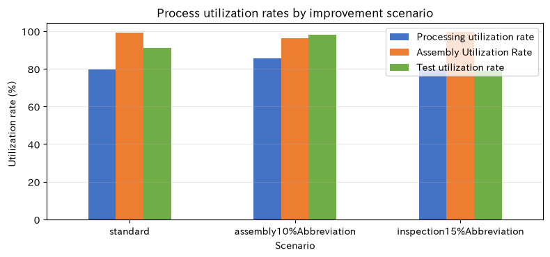
will be updated. Processing time $P_{j,k}$ is a log-normal distribution, and failure stops are added with a certain probability. Compare three options: standard, 10% shorter assembly, and enhanced inspection using the same random number series.

Check with Python

def line_sim(scenario, seed, jobs=240):
    line_rng = np.random.default_rng(seed)
    means = np.array([18.0, 25.0, 21.0])
    if scenario == "assembly10%Abbreviation":
        means[1] *= 0.90
    if scenario == "inspection15%Abbreviation":
        means[2] *= 0.85
    durations = line_rng.lognormal(np.log(means), [0.18, 0.14, 0.22], size=(jobs, 3))
    failures = line_rng.random((jobs, 3)) < [0.025, 0.015, 0.035]
    durations += failures * line_rng.uniform(20, 55, size=(jobs, 3))
    completion = np.zeros((jobs, 3))
    busy = durations.sum(axis=0)
    for j in range(jobs):
        for k in range(3):
            prev_job = completion[j - 1, k] if j else 0
            prev_stage = completion[j, k - 1] if k else 0
            completion[j, k] = max(prev_job, prev_stage) + durations[j, k]
    makespan = completion[-1, -1]
    return makespan, jobs / (makespan / 450), busy / makespan, completion

line_rows = []
line_completion = {}
for scenario in ["standard", "assembly10%Abbreviation", "inspection15%Abbreviation"]:
    makespan, daily, utilization, completion = line_sim(scenario, SEED + 87)
    line_rows.append([scenario, makespan, daily, *utilization])
    line_completion[scenario] = completion
line_result = pd.DataFrame(line_rows, columns=["Scenario", "completion_time_minutes", "nissan_equivalent_platform", "Processing utilization rate", "Assembly Utilization Rate", "Test utilization rate"])
display(line_result)

fig, ax = plt.subplots(figsize=(8, 3.8))
plot_data = line_result.set_index("Scenario")[["Processing utilization rate", "Assembly Utilization Rate", "Test utilization rate"]] * 100
plot_data.plot.bar(ax=ax, color=["#4472C4", "#ED7D31", "#70AD47"], rot=0)
ax.set_title("Process utilization rates by improvement scenario")
ax.set_xlabel("Scenario")
ax.set_ylabel("Utilization rate (%）")
ax.grid(axis="y", alpha=0.3)
plt.tight_layout()
plt.show()

	Scenario	completion_time_minutes	nissan_equivalent_platform	Processing utilization rate	Assembly Utilization Rate	Test utilization rate
0	standard	6,127.66	17.62	0.80	0.99	0.91
1	assembly10%Abbreviation	5,698.83	18.95	0.86	0.96	0.98
2	inspection15%Abbreviation	6,124.45	17.63	0.80	0.99	0.79

png

Reading the results

The cycle shortening rate and the daily improvement rate do not match. Even if you improve anything other than the constrained process, the effect on the overall completion time is limited. While considering processes with high utilization rates as candidates for improvement, we also check for long stoppages due to breakdowns and work-in-progress between processes. In investment decisions, the average and downward percentiles of multiple iterations are compared with the cost per unit per additional production unit.

No.088: Supply Chain Simulation — Choosing Buffers for Supply Disruptions

Meaning in Practice

Supplier stoppages for key components can cause factory shortages after a few days’ delay, further affecting customer delivery deadlines. Safety stock, alternative procurement, and express shipping enhance resilience but come with peacetime costs. You can use BCP not just to be safe, but to compare out-of-stock ratios and costs.

Approach to Analysis and Modeling

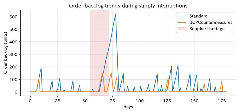
We manage incoming goods from suppliers to factories as lead-time events, allocation of daily demand from factory inventory. During the outage period, regular orders do not arrive, and the countermeasure allows for higher order points and alternative procurement in case of out-of-stock items. Evaluation indicators include fulfillment rate, maximum order backlog, annual total cost, and number of days to recover after interruption.

Check with Python

def supply_chain_sim(policy, seed, days=180):
    sc_rng = np.random.default_rng(seed)
    on_hand, backlog = 280, 0
    pipeline = []
    total_demand = immediate_total = holding = expedite = 0
    max_backlog = 0
    history = []
    R, Q = ((180, 260) if policy == "Standard" else (280, 320))
    for day in range(days):
        arrivals = sum(q for due, q in pipeline if due == day)
        pipeline = [(due, q) for due, q in pipeline if due > day]
        on_hand += arrivals
        demand = int(sc_rng.poisson(42))
        total_demand += demand
        old_backlog = backlog
        immediate_total += min(demand, max(0, on_hand - old_backlog))
        requested = old_backlog + demand
        shipped = min(on_hand, requested)
        on_hand -= shipped
        backlog = requested - shipped
        inventory_position = on_hand + sum(q for _, q in pipeline) - backlog
        disruption = 55 <= day < 72
        if inventory_position <= R and not disruption:
            pipeline.append((day + int(sc_rng.integers(5, 10)), Q))
        if policy == "BCPCountermeasures" and backlog > 80:
            emergency = min(120, backlog)
            pipeline.append((day + 2, emergency))
            expedite += emergency
        holding += on_hand
        max_backlog = max(max_backlog, backlog)
        history.append([day, on_hand, backlog])
    cost = holding * 28 + backlog * 1800 + expedite * 650
    hist = pd.DataFrame(history, columns=["days", "factory inventory", "unfinished order"])
    after = hist.loc[hist["days"] >= 72]
    recovered = after.loc[after["unfinished order"] <= 5, "days"]
    recovery_days = (recovered.iloc[0] - 72) if len(recovered) else np.nan
    return immediate_total / total_demand, max_backlog, cost, recovery_days, hist

sc_rows, sc_hist = [], {}
for policy in ["Standard", "BCPCountermeasures"]:
    fill, max_b, cost, recovery, hist = supply_chain_sim(policy, SEED + 88)
    sc_rows.append([policy, fill, max_b, cost, recovery])
    sc_hist[policy] = hist
supply_result = pd.DataFrame(sc_rows, columns=["Policy", "Immediate Payment Satisfaction Rate", "Maximum Order Backlog", "total_cost_yen", "Days to recover after interruption"])
display(supply_result)

fig, ax = plt.subplots(figsize=(8, 3.8))
for policy, hist in sc_hist.items():
    ax.plot(hist["days"], hist["unfinished order"], label=policy)
ax.axvspan(55, 72, color="#C00000", alpha=0.12, label="Supplier shortage")
ax.set_title("Order backlog trends during supply interruptions")
ax.set_xlabel("days")
ax.set_ylabel("Order backlog (units)")
ax.grid(alpha=0.3)
ax.legend()
plt.tight_layout()
plt.show()

	Policy	Immediate Payment Satisfaction Rate	Maximum Order Backlog	total_cost_jpy	Days to recover after interruption
0	Standard	0.64	621	277452	9
1	BCPCountermeasures	0.88	152	1448626	4

png

Reading the results

BCP measures increase weektime inventory and express expenses, but also reduce the maximum order backlog and recovery time during interruptions. You select not only average annual costs, but also key customer downtime losses and contract penalties. Since a single fixed outage can lead to biased conclusions, stress tests that vary the timing and duration of occurrences and simultaneous damage to multiple suppliers are necessary.

No.089: Demand Simulation — Comparing S&OP Capability Proposals with Probabilism

Meaning in Practice

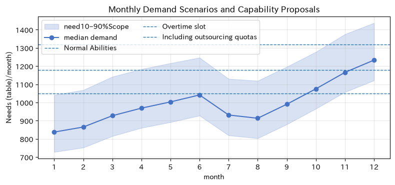
Even if the sales forecast is 1,000 units per month, performance fluctuates depending on promotional effects, seasonality, and the number of large projects. Matching capacity to the forecast average increases overtime and out-of-stock during busy months. S&OP uses demand scenarios and agrees on combinations of usual capability, overtime, and outsourcing.

Approach to Analysis and Modeling

Demand for $t$ months

$D_t=(L+T_t)S_t+M_t+\varepsilon_t$

For example, $L$ is standard demand, $T$ is trend, $S$ is seasonal coefficient, $M$ is promotional or large-scale projects, and $\varepsilon$ is usually fluctuating. Generate 1,000 annual passes and evaluate the probability of ability exceedance and annual shortfall by ability type.

Check with Python

demand_rng = np.random.default_rng(SEED + 89)
n_paths, months = 3000, 12
season = np.array([0.90, 0.92, 0.98, 1.02, 1.05, 1.08, 0.95, 0.93, 1.00, 1.08, 1.16, 1.22])
trend = np.arange(months) * 8
base = (900 + trend) * season
noise = demand_rng.normal(0, 75, size=(n_paths, months))
campaign = (demand_rng.random((n_paths, months)) < 0.16) * demand_rng.normal(180, 45, (n_paths, months))
large_order = (demand_rng.random((n_paths, months)) < 0.08) * demand_rng.integers(180, 380, (n_paths, months))
demand_paths = np.maximum(0, base + noise + campaign + large_order)

capacity_options = {"Normal Abilities": 1050, "Overtime slot": 1180, "Including outsourcing quotas": 1320}
demand_rows = []
for name, cap in capacity_options.items():
    shortage = np.maximum(0, demand_paths - cap)
    demand_rows.append([name, cap, (demand_paths > cap).mean(), shortage.sum(axis=1).mean(), np.quantile(shortage.sum(axis=1), 0.95)])
demand_result = pd.DataFrame(demand_rows, columns=["capability plan", "moon_ability_platform", "Monthly ability exceeds probability", "average_annual_shortfall_platform", "annual shortage95%position_platform"])
display(demand_result)

q10, q50, q90 = np.quantile(demand_paths, [0.1, 0.5, 0.9], axis=0)
fig, ax = plt.subplots(figsize=(8, 3.8))
ax.fill_between(np.arange(1, 13), q10, q90, color="#4472C4", alpha=0.2, label="need10–90%Scope")
ax.plot(np.arange(1, 13), q50, color="#4472C4", marker="o", label="median demand")
for name, cap in capacity_options.items():
    ax.axhline(cap, linestyle="--", linewidth=1, label=name)
ax.set_title("Monthly Demand Scenarios and Capability Proposals")
ax.set_xlabel("month")
ax.set_ylabel("Needs (table)/month)")
ax.set_xticks(range(1, 13))
ax.grid(alpha=0.3)
ax.legend(ncol=2)
plt.tight_layout()
plt.show()

	capability plan	moon_ability_platform	Monthly ability exceeds probability	average_annual_shortfall_platform	annual shortage95%position_platform
0	Normal Abilities	1050	0.38	670.75	1,188.59
1	Overtime slot	1180	0.18	242.43	613.50
2	Including outsourcing quotas	1320	0.05	65.70	289.95

png

Reading the results

Even if the median is within capacity, there will be shortfalls at the upper end of the demand distribution. Normal capacity is treated as fixed cost, overtime and outsourcing as variable costs, and the probability of overcapacity and the tolerance for shortfall costs are agreed upon. Since promotional and large-scale deals are not pure random numbers but linked to sales activities, scenarios based on project accuracy are set jointly with the sales department and updated monthly.

No.090: Digital Twin — Updating status and proactively evaluating measures at on-site events

Meaning in Practice

Digital twins are not just 3D displays themselves; they synchronize the current state of the site with data and compare future scenarios from that state. If standard time remains outdated, even sophisticated models can make mistakes. We update the model based on daily cycle performance and provide the expected completion of the remaining balance for the day.

Approach to Analysis and Modeling

The estimated cycle time of process $k$ is achieved exponentially smoothing by the observation $y_{k,t}$ ,

$\hat\mu_{k,t}=\alpha y_{k,t}+(1-\alpha)\hat\mu_{k,t-1}$

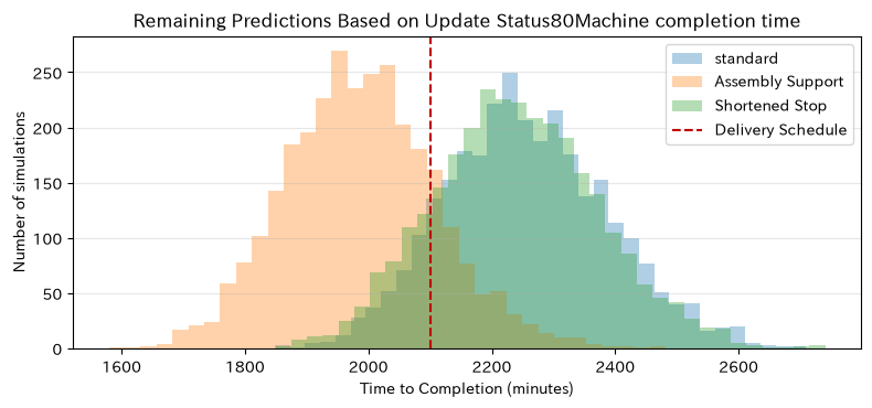
I will update you. The minimum configuration consists of (1) target KPIs, (2) state data, (3) update rules, (4) future simulations, (5) decision-making, and (6) verification based on actual results. Using the current estimate as the initial state, we compare the criteria, support, and shortened stop proposals.

Check with Python

twin_rng = np.random.default_rng(SEED + 90)
standards = {"processing": 18.0, "assembly": 25.0, "inspection": 21.0}
events = []
for machine, standard in standards.items():
    drift = {"processing": 1.03, "assembly": 1.12, "inspection": 0.98}[machine]
    observed = twin_rng.lognormal(np.log(standard * drift), 0.12, 40)
    events.extend([[machine, i + 1, value] for i, value in enumerate(observed)])
event_data = pd.DataFrame(events, columns=["Project", "order of completion", "achievements_ct"])

alpha = 0.20
state_rows = []
for machine, group in event_data.groupby("Project", sort=False):
    estimate = standards[machine]
    for value in group["achievements_ct"]:
        estimate = alpha * value + (1 - alpha) * estimate
    state_rows.append([machine, standards[machine], estimate, estimate / standards[machine] - 1])
twin_state = pd.DataFrame(state_rows, columns=["Project", "standard_ct_points", "update_ct_minutes", "standard deviation rate"]).set_index("Project")
display(twin_state)

def twin_forecast(ct, scenario, seed, remaining=80, reps=3000):
    r = np.random.default_rng(seed)
    adjusted = ct.copy()
    downtime_mean = 38
    if scenario == "Assembly Support":
        adjusted["assembly"] *= 0.88
    if scenario == "Shortened Stop":
        downtime_mean = 22
    bottleneck_ct = max(adjusted.values())
    finish = remaining * r.lognormal(np.log(bottleneck_ct), 0.06, reps) + r.gamma(2, downtime_mean / 2, reps)
    return finish

ct_now = twin_state["update_ct_minutes"].to_dict()
twin_rows, twin_samples = [], {}
for i, scenario in enumerate(["standard", "Assembly Support", "Shortened Stop"]):
    samples = twin_forecast(ct_now, scenario, SEED + 900 + i)
    twin_samples[scenario] = samples
    twin_rows.append([scenario, samples.mean(), np.quantile(samples, 0.90), (samples <= 2100).mean()])
twin_result = pd.DataFrame(twin_rows, columns=["Scenario", "average_estimated_completion_in_minutes", "completed90%quantile", "2100Completion Probability Within Minutes"])
display(twin_result)

fig, ax = plt.subplots(figsize=(8, 3.8))
for scenario, samples in twin_samples.items():
    ax.hist(samples, bins=35, alpha=0.35, label=scenario)
ax.axvline(2100, color="#C00000", linestyle="--", label="Delivery Schedule")
ax.set_title("Remaining Predictions Based on Update Status80Machine completion time")
ax.set_xlabel("Time to Completion (minutes)")
ax.set_ylabel("Number of simulations")
ax.grid(axis="y", alpha=0.3)
ax.legend()
plt.tight_layout()
plt.show()

	StandardCT_minutes	UpdateCT_minutes	standard deviation rate
Project
processing	18.00	18.70	0.04
assembly	25.00	27.68	0.11
inspection	21.00	20.09	-0.04

	Scenario	average_estimated_completion_in_minutes	completed90%position_minutes	2100Completion Probability Within Minutes
0	standard	2,257.37	2,433.68	0.12
1	Assembly Support	1,987.86	2,138.01	0.83
2	Shortened Stop	2,239.69	2,412.84	0.15

png

Reading the results

Processes with a high standard deviation rate serve as signals to examine deterioration, product composition, and changes in work methods. By calculating the on-deadline completion probability from the updated state, you can compare cheering and stoppage shortening on the same scale. In production, we continuously monitor prediction errors and detect sensor defects or time deviations. Even with automated suggestions, approval permissions for manufacturing orders, manual operation when models are stopped, and change histories are clearly defined.

Practical Implications Seen Through Target Exercise

Choose time expressions that fit the question: For total profit distribution, Monte Carlo is suitable; for process order, discrete events are suitable; for inter-agent interactions, agent-based is suitable.
From the average to the distribution: In addition to average profit and average demand, the probability of deficits, downward percentiles, and the probability of exceeding capacity are used in decision-making.
Not aiming for high utilization: In queues, the number of people in wait increases nonlinearly as usage increases. We list both the delivery service and the cost.
Localized improvements overallKPIEvaluate by: Process reduction, preventive maintenance, and safety inventory are compared in terms of effectiveness in throughput, stoppage, and total cost.
Clearly indicate the time delay: There are delays in capacity adjustment, ordering, and supply disruptions. Monthly aggregation alone overlooks vibrations and ripples.
Close the model to on-site performance: Digital twins operate as a single update cycle involving state synchronization, future comparison, and performance verification.

What is necessary for practical implementation

1. Define decision-making, scope, and KPIs in advance

Instead of starting with “recreating the entire factory,” define who decides what and when—such as the number of inspectors, ordering points, overtime slots, and alternative procurement. KPIs include not only averages but also on-time delivery rates, around the 95th percentile, maximum order backlog, and total costs.

2. Manage input data and business rules

Item, process, equipment, shifts, arrangements, order backlogs, reasons for stoppages, and definitions of orders received and lost orders are all gathered. Record and reproducibly record data extraction date and time, units, missing compensation, and start date for standard time application.

3. Validation is conducted step by step

We check event order and inventory balance individually, reproduce past periods, and have on-site staff identify extreme cases. In addition to ensuring the model’s values match actual results, we also verify that the direction of cause and effect aligns with on-site knowledge.

4. Operate from small decision-making loops

For each component and process, “data updates→ scenario comparison→ approval →→ execution performance evaluation” are rotated to measure effects such as decision time and shortage reduction. After that, the scope of integration with ERP, MES, equipment, and procurement data will be expanded.

5. Communicate uncertainty and the boundary of responsibility

Forecast sections, assumptions, and non-applicable conditions are displayed on the screen and meeting materials. Includes acceptance or rejection of automated proposals, emergency overwrite permissions, alternative procedures when the model stops, and audit logs in business design.

Conclusion

From No.081 to No.090, we covered Monte Carlo assessments of profit risks, process events, interactions between equipment and maintenance personnel, queues, supply-demand feedback, inventory policies, production lines, supply disruptions, demand scenarios, and performance-linked digital twins.

The value of simulation lies not in creating complex models, but in comparing the outcomes and risks of options before execution. Verify income and expenses and events on a small scale, gradually adding only the elements necessary for decision-making. By continuously leaving gaps between predictions and actual results, the model can be developed from a one-time analysis into a decision-making foundation on the ground.

Consultations for Corporations

At Surikoubo, we offer consultations for everything from simulation in manufacturing, inventory, production, and supply chain design, to planning digital twins and support for implementation and in-house production.

Discrete Event Simulation Targeting Processes, Logistics, and Maintenance
Monte Carlo assessment and scenario design for demand, supply, and profit risks
Comparative verification of inventory policies, personnel allocation, capital investment, and BCP initiatives
Digital twin / decision-making platform connecting ERP, MES, and facility data
Corporate training covering Python, statistics, and simulation

📩 Contact Us: surikobo.co.jp/contact
Please feel free to consult us first.

Learning Manufacturing Simulation with Python | 10 Exercises from Monte Carlo to Digital Twins

Factory Management That Anticipates Fluctuations: 10 Exercise-Down Simulations for Industrial Pump Factories

Introduction: Practical Challenges in Manufacturing Covered in This Article

Common situations on site

Why is this issue so difficult to judge?

Overview of Exercise covered this time

Preparing the Python environment

Creation of Fictional Data

No.081: Monte Carlo — Measuring the Downside of Annual Profits by Probability

Meaning in Practice

Approach to Analysis and Modeling

Check with Python

Reading the results

No.082: Discrete Event — Recreating Process Competition and Job Waiting

Meaning in Practice

Approach to Analysis and Modeling

Check with Python

Reading the results

No.083: Agent-Based — Capturing Local Decisions and Equipment Behavior by Security Personnel

Meaning in Practice

Approach to Analysis and Modeling

Check with Python

Reading the results

No.084: Queue — Determining the Number of Final Inspection Personnel Based on Service Level

Meaning in Practice

Approach to Analysis and Modeling

Check with Python

Reading the results

No.085: System Dynamics — Viewing Backlog and Ability Adjustment Feedback

Meaning in Practice

Approach to Analysis and Modeling

Check with Python

Reading the results

No.086: Inventory Simulation — Comparing Order Points and Order Quantities by Cost and Fulfillment Rate

Meaning in Practice

Approach to Analysis and Modeling

Check with Python

Reading the results

No.087: Production Line Simulation — Comparing Bottleneck Improvement Proposals

Meaning in Practice

Approach to Analysis and Modeling

Check with Python

Reading the results

No.088: Supply Chain Simulation — Choosing Buffers for Supply Disruptions

Meaning in Practice

Approach to Analysis and Modeling

Check with Python

Reading the results

No.089: Demand Simulation — Comparing S&OP Capability Proposals with Probabilism

Meaning in Practice

Approach to Analysis and Modeling

Check with Python

Reading the results

No.090: Digital Twin — Updating status and proactively evaluating measures at on-site events

Meaning in Practice

Approach to Analysis and Modeling

Check with Python

Reading the results

Practical Implications Seen Through Target Exercise

What is necessary for practical implementation

1. Define decision-making, scope, and KPIs in advance

2. Manage input data and business rules

3. Validation is conducted step by step

4. Operate from small decision-making loops

5. Communicate uncertainty and the boundary of responsibility

Conclusion

Consultations for Corporations

Related Posts

Practical Manufacturing DI with Python | KPI, Knowledge Graphs, Optimization, and AI Agent: 10 Exercise-On Steps

Learning Manufacturing Decision Science with Python | 10 Key Exercises on Expected Value, Bayes, and Robust Optimization

Hands-on Machine Learning in Manufacturing with Python | 10 Exercise-Down Prediction, Causal Inference, and Optimization

Practical Customer Analysis in Manufacturing Using Python | 10 Exercises on RFM, Defection, CLV, and Uplift

Learning Production Planning in Manufacturing with Python | From Line Balancing to Digital Twin: 10 Exercises