Manufacturing Performance Management Connecting CSV to Dashboards — 10 Exercise-Down Business System Functions

Focusing on the Daily Production Performance Management of the manufacturing floor, we design CSV uploads, database registration, pagination, multiple condition and date range searches, aggregation APIs, graph APIs, dashboards, forms, and batch processing all in one succession. Not only do we create individual functions, but we also verify the process from which input data becomes a decision-making tool for management and the field, using fictional data and Python.

The target is the No.081〜No.090 of 100 system development exercises.

[!NOTE] This material is a notebook previously used by Surikoubo (or personally by the representative, Kazuyama), and has been reconstructed, edited, and published with the company’s permission.
All data listed is fictional and has no relation whatsoever to real companies, factories, or figures.

Introduction: Practical Challenges in Manufacturing Covered in This Article

In factories, production performance obtained from equipment and on-site terminals is collected as CSV, registered in business systems, and sometimes deployed to morning meeting lists, administrator dashboards, and monthly reports. If column names fluctuate, duplicate registrations occur, search delays, or mismatches in aggregation definitions occur during this process, even if the numbers are from the same factory, the screen and the form do not match.

In this notebook, you not only check whether you can import it, but also manage Integrity, uniqueness, timeliness, and traceability. The ultimate goal is not to increase the number of screens, but to support decisions related to quality, delivery time, and operation through reproducible data processing.

Common situations on site

• Each site has different CSV column names and character encodings, and the staff manually corrects them.
• Re-uploading results in duplicate registration of the same achievement
• The list grows to tens of thousands, and display and search take time
• Screens, aggregations, and reports are calculated under different conditions, and the values do not match.
• Date boundaries, night shifts, and time zone handling are ambiguous, causing daily performance to be misaligned.
• Failing to notice batch failures until the next morning and starting meetings with old KPIs

Why is this issue so difficult to judge?

The quality of business systems cannot be evaluated by the normal system screens alone. It is important to provide accurate figures by business deadlines, including large volumes, missing items, duplicates, delays, partial failures, and reruns. Also, even the single ‘defect rate’ can change depending on whether the denominator is input, number completed, or number of inspections.

So, replace functional requirements with the following KPIs.

$$\text{import success rate} = \frac{\text{number of lines that can be registered}}{\text{number of received lines}}, \quad \text{defect rate} = \frac{\text{number of defects}}{\text{number of good products} + \text{number of defects}}, \quad \text{On-time batch completion rate} = \frac{\text{number of successful completions before deadline}}{\text{planned execution}}$$

Treating functions, data definitions, performance, and operations as the same design object helps reduce errors in decision-making.

Overview of Exercise covered this time

No.	Theme	Key Points to Check in Manufacturing Performance Management
081	CSV Upload	Entrance inspection of type, size, and required rows
082	Registering CSV data in the database	Verification, deduplication, transactions
083	pagination	Stable viewing of bulk statements
084	Multiple Condition Search	Narrowing down according to on-site investigation procedures
085	Date Range Search	Definition of Periods Including Boundaries and Night Shifts
086	Aggregation API	Centralized KPI definitions
087	API for graph display	Easy-to-draw time-series data
088	dashboard	The path from anomaly detection to detailed confirmation
089	Forms and Reports	Saving definite values, editions, and output conditions
090	batch processing	Scheduled execution, reexecution, monitoring

Data flows in the order of “Entry → Persistence → Search → Aggregation & Visualization → Distribution & Regular Execution.”

Preparing the Python environment

Data is handled pandas and numpy, and visualized by matplotlib. Japanese is displayed using japanize_matplotlib. It does not connect to external services or data, and instead fixes random number seeds. Here, Python processing is not the web implementation itself, but rather a small verification of the business rules that should be implemented in APIs or databases.

%matplotlib inline
%config InlineBackend.figure_format = 'svg'

import sys
import json
import hashlib
from io import StringIO
import numpy as np
import pandas as pd
import matplotlib
import matplotlib.pyplot as plt
import japanize_matplotlib
from IPython.display import display

SEED = 20260712
rng = np.random.default_rng(SEED)
pd.set_option("display.max_columns", 20)
pd.set_option("display.width", 140)
print("Python:", sys.version.split()[0])
print("pandas:", pd.__version__, "numpy:", np.__version__, "matplotlib:", matplotlib.__version__)
print("seed:", SEED)

Python: 3.13.1
pandas: 3.0.3 numpy: 2.5.1 matplotlib: 3.11.0
seed: 20260712

Creation of Fictional Data

From April to June 2026, 1,800 production records will be generated for 3 factories and 6 lines. Each row has its own performance ID, completion date and time, factory, line, part number, number of good products, number of defects, stop time, and registry source. For CSV import tests, in addition to normal rows, we intentionally include missing required values, quantity mismatches, and duplicates.

In production, it is necessary to agree with the business departments on the entities responsible for obtaining production performance IDs, synchronizing equipment time, correcting history, and shift boundaries.

n = 1800
start = pd.Timestamp("2026-04-01 00:00")
completed_at = start + pd.to_timedelta(rng.integers(0, 91 * 24 * 60, n), unit="m")
factory = rng.choice(["East Factory", "West Factory", "Central Factory"], n, p=[0.40, 0.35, 0.25])
line_map = {"East Factory": ["E-1", "E-2"], "West Factory": ["W-1", "W-2"], "Central Factory": ["C-1", "C-2"]}
line = [rng.choice(line_map[f]) for f in factory]
good = rng.integers(70, 241, n)
base_defect = np.where(np.array(line) == "W-2", 0.030, 0.015)
defect = rng.binomial(np.maximum(good, 1), base_defect)

production = pd.DataFrame({
    "result_id": [f"PR-{i:06d}" for i in range(1, n + 1)],
    "completed_at": completed_at,
    "factory": factory,
    "line": line,
    "product": rng.choice(["AX-100", "AX-200", "BZ-310", "CZ-500"], n),
    "good_qty": good,
    "defect_qty": defect,
    "downtime_min": np.round(rng.gamma(1.4, 8.0, n), 1),
    "source": rng.choice(["Facility Integration", "on-site terminal", "CSV"], n, p=[0.55, 0.30, 0.15]),
}).sort_values(["completed_at", "result_id"]).reset_index(drop=True)
production["total_qty"] = production["good_qty"] + production["defect_qty"]
production["defect_rate_pct"] = production["defect_qty"] / production["total_qty"] * 100

upload_sample = production.sample(115, random_state=SEED).copy()
upload_sample = pd.concat([upload_sample, upload_sample.iloc[[0, 1]]], ignore_index=True)
upload_sample.loc[3, "factory"] = None
upload_sample.loc[7, "good_qty"] = -5

display(production.head())
print("Production Record:", production.shape, "Period:", production.completed_at.min(), "〜", production.completed_at.max())
print("Number of Upload Test Rows:", len(upload_sample))

	result_id	completed_at	factory	line	product	good_qty	defect_qty	downtime_min	source	total_qty	defect_rate_pct
0	PR-001150	2026-04-01 00:40:00	East Factory	E-1	BZ-310	211	1	4.6	CSV	212	0.471698
1	PR-000624	2026-04-01 00:58:00	East Factory	E-1	CZ-500	117	4	14.8	CSV	121	3.305785
2	PR-001316	2026-04-01 01:13:00	West Factory	W-1	BZ-310	218	3	21.6	CSV	221	1.357466
3	PR-000365	2026-04-01 01:38:00	East Factory	E-1	AX-200	173	1	4.8	Facility Integration	174	0.574713
4	PR-001490	2026-04-01 02:27:00	Central Factory	C-2	AX-200	106	1	17.3	CSV	107	0.934579

Production record: (1800, 11) Period: 2026-04-01 00:40:00 〜 2026-06-30 22:36:00
Number of Upload Test Lines: 117

No.081: Creating a CSV Upload Feature

Meaning in Practice

Uploading is the boundary where external data enters the system. Don’t trust only the file name; check the file extension, size, character encoding, header, and line count, and return the processing acceptance ID. For large files, synchronization does not make you wait; after reception, asynchronous processing is performed so users can check progress and errors in a design that is ideal.

Approach to Analysis and Modeling

Separate entry inspections from row-by-line operational inspections. Here, the difference between the required column set $R$ and the received column set $C$ is calculated $R-C$; if it is missing, processing does not start. When accepting the request, you can save the hash of the file contents to detect resending the same file.

Check with Python

required = {"result_id", "completed_at", "factory", "line", "product", "good_qty", "defect_qty"}
csv_text = upload_sample.to_csv(index=False)
received = pd.read_csv(StringIO(csv_text))
missing_columns = sorted(required - set(received.columns))
file_hash = hashlib.sha256(csv_text.encode("utf-8")).hexdigest()[:16]
upload_check = pd.DataFrame({
    "Examination": ["File size", "Number of lines", "required column", "Content hash"],
    "Results": [f"{len(csv_text.encode('utf-8')):,} bytes", f"{len(received):,} rows", "OK" if not missing_columns else str(missing_columns), file_hash],
    "Judgment": ["OK", "OK", "OK" if not missing_columns else "NG", "Records"],
})
display(upload_check)

	Examination	Results	Judgment
0	File size	11,174 bytes	OK
1	Number of lines	117 rows	OK
2	required column	OK	OK
3	Content hash	60b1f4d6aa6d7e9d	Records

Reading the results

Since the required columns are in place, proceed to row-by-row verification. On the other hand, the existence of a column does not guarantee that the value is correct. Save the receipt ID, hash, recipient, and receipt time, and decide whether to reject the same file if it is resent: “Reject,” “Show previous result,” or “Explicitly reprocess.” CSV injection and oversized files are also addressed at the entrance.

No.082: Registering CSV Data in the Database

Meaning in Practice

With database registration, only part of the data is registered, preventing inconsistencies in numbers. The method of excluding invalid lines and registering only the normal line, or restoring even one invalid line, is chosen according to the deadline and correction procedure of the operation.

Approach to Analysis and Modeling

The Achievement ID is used as the unique key to verify required values, non-negative quantities, and overlaps with existing IDs. It is important to Idempotency that the results do not multiply even after re-running. In databases, unique constraints and transactions serve as the last line of defense, and do not rely solely on application-side inspection.

Check with Python

staging = upload_sample.copy()
staging["Missing essential value"] = staging[["result_id", "completed_at", "factory", "line", "product"]].isna().any(axis=1)
staging["Quantity misalignment"] = staging["good_qty"].lt(0) | staging["defect_qty"].lt(0)
staging["file duplication"] = staging.duplicated("result_id", keep=False)
staging["Registration Approval or Failure"] = ~(staging[["Missing essential value", "Quantity misalignment", "file duplication"]].any(axis=1))
validation = staging[["Missing essential value", "Quantity misalignment", "file duplication"]].sum().rename("Number of Relevant Lines").to_frame()
validation.loc["Registrable", "Number of Relevant Lines"] = staging["Registration Approval or Failure"].sum()
display(validation.astype(int))
display(staging.loc[~staging["Registration Approval or Failure"], ["result_id", "factory", "good_qty", "Missing essential value", "Quantity misalignment", "file duplication"]])

	Number of Relevant Lines
Missing essential value	1
Quantity misalignment	1
file duplication	4
Registrable	111

	result_id	factory	good_qty	Missing essential value	Quantity misalignment	file duplication
0	PR-001092	West Factory	121	False	False	True
1	PR-001300	West Factory	86	False	False	True
3	PR-001520	NaN	192	True	False	False
7	PR-000098	East Factory	-5	False	True	False
115	PR-001092	West Factory	121	False	False	True
116	PR-001300	West Factory	86	False	False	True

Reading the results

If you provide the error reason along with the line number, item name, and example correction, the person in charge can correct the original file. Simply deleting duplicate lines causes missing correction data with different contents, so the same ID and content are separated from those with the same ID but different content. Production registration is verified using staging tables, and only finalized after reconciling audit logs and case counts.

No.083: Implementing Pagination on the List Screen

Meaning in Practice

Sending large volumes of invoices at once puts a load on the DB, API, and browser. Pagination not only speeds up display but also allows users to maintain their research position and recheck in the same order.

Approach to Analysis and Modeling

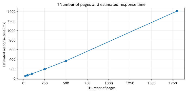
While LIMIT/OFFSET is easier to implement, deeper pages tend to cause more skipping, and rows may shift when adding new pages while viewing. Consider a cursor system that uses stable composite sort keys. Here, assuming 50 items per page, we compare the number of forwarded lines with the estimated response time.

Check with Python

page_sizes = np.array([25, 50, 100, 250, 500, 1800])
pagination = pd.DataFrame({"1Number of pages": page_sizes})
pagination["estimated_response_time_ms"] = np.round(35 + page_sizes * 0.55 + (page_sizes / 100) ** 1.5 * 5).astype(int)
pagination["estimated_transfer_volume_kb"] = np.round(page_sizes * 0.72, 1)
display(pagination)
fig, ax = plt.subplots(figsize=(8, 4))
ax.plot(pagination["1Number of pages"], pagination["estimated_response_time_ms"], marker="o")
ax.set_title("1Number of pages and estimated response time")
ax.set_xlabel("1Number of pages")
ax.set_ylabel("Estimated response time (ms）")
ax.grid(True, alpha=0.3)
plt.tight_layout(); plt.show()

	1Number of pages	estimated_response_time_ms	estimated_transfer_volume_KB
0	25	49	18.0
1	50	64	36.0
2	100	95	72.0
3	250	192	180.0
4	500	366	360.0
5	1800	1407	1296.0

Reading the results

The more pages you have, the fewer repeat trips you get, but the initial display and transfer volume will increase. We select 50 to 100 initial candidates based on actual measurements. APIs define a unique order like completed_at DESC, result_id DESC, and if calculating total counts is costly, you can design it to display approximate numbers or return only “Next page available.”

No.084: Implementing Multiple Condition Search

Meaning in Practice

Quality personnel combine conditions such as “West Factory, W-2, AX-200, defect rate 2% or higher” to identify the scope of the abnormality. Search criteria should not be arranged in a database column, but rather matched to the on-site survey procedures and terminology.

Approach to Analysis and Modeling

Conditions between conditions are usually defined as AND, and multiple values of the same item are defined as OR. It parameterizes free strings without concatenating them into SQL. Usage frequency and selectivity are measured from search logs, and composite indexes are designed based on frequency conditions and sorting order.

Check with Python

steps = []
searched = production.copy(); steps.append(("all items", len(searched)))
searched = searched[searched.factory.eq("West Factory")]; steps.append(("West Factory", len(searched)))
searched = searched[searched.line.eq("W-2")]; steps.append(("W-2", len(searched)))
searched = searched[searched["product"].isin(["AX-100", "AX-200"])]; steps.append(("Eligibility2Product Number", len(searched)))
searched = searched[searched.defect_rate_pct.ge(2.0)]; steps.append(("non_performing_rate2%That's all.", len(searched)))
funnel = pd.DataFrame(steps, columns=["After Conditions Applied", "number_of_cases"])
funnel["total_package_ratio_pct"] = (funnel["number_of_cases"] / len(production) * 100).round(1)
display(funnel)
display(searched.nlargest(5, "defect_rate_pct")[["result_id", "completed_at", "product", "good_qty", "defect_qty", "defect_rate_pct"]].round(2))

	After Conditions Applied	number_of_cases	total_package_ratio_pct
0	all items	1800	100.0
1	West Factory	612	34.0
2	W-2	291	16.2
3	Eligibility2Product Number	142	7.9
4	non_performing_rate2%That's all.	104	5.8

/var/folders/3y/fmw40k0x78xblvb3gkcyvy1h0000gn/T/ipykernel_45011/1531514336.py:10: UserWarning: obj.round has no effect with datetime, timedelta, or period dtypes. Use obj.dt.round(...) instead.
  display(searched.nlargest(5, "defect_rate_pct")[["result_id", "completed_at", "product", "good_qty", "defect_qty", "defect_rate_pct"]].round(2))

	result_id	completed_at	product	good_qty	defect_qty	defect_rate_pct
358	PR-000029	2026-04-19 17:01:00	AX-100	105	9	7.89
761	PR-000391	2026-05-09 13:45:00	AX-200	196	13	6.22
65	PR-001092	2026-04-04 04:18:00	AX-200	121	8	6.20
187	PR-000723	2026-04-10 06:34:00	AX-200	108	7	6.09
436	PR-000704	2026-04-22 19:37:00	AX-100	92	5	5.15

Reading the results

By showing the number of cases by stage, you can explain which conditions are being targeted. If there are zero cases, the UI that allows relaxation while maintaining the conditions is enabled. The search API defines allowed items, operators, and maximum durations to prevent overload from unlimited ambiguous searches. Sharing frequently used conditions as saved searches improves the reproducibility of morning meetings.

No.085: Implementing Date Range Search

Meaning in Practice

In factories with night shifts beyond midnight, the calendar day and production date do not match. If you set ‘June 1st’ as 0:00–24:00, the night shift performance will be split into different days. It is necessary to unify the meaning of dates and times across screens, APIs, and databases.

Approach to Analysis and Modeling

If the period is set to a half-open interval $[start, end)$ that includes the start but not the end, you can avoid overlapping adjacent periods. Here, the production day boundary is defined as 8 a.m., and the completed_at - 8hours date is defined as the production date. In the database, the basic design is to save UTC and convert it to the factory time zone when displaying.

Check with Python

boundary_sample = pd.DataFrame({
    "completed_at": pd.to_datetime(["2026-06-01 00:30", "2026-06-01 07:59", "2026-06-01 08:00", "2026-06-01 23:30", "2026-06-02 07:59"])
})
boundary_sample["calendar day"] = boundary_sample.completed_at.dt.date
boundary_sample["production_date_value_8"] = (boundary_sample.completed_at - pd.Timedelta(hours=8)).dt.date
display(boundary_sample)

start_at, end_at = pd.Timestamp("2026-06-01 08:00"), pd.Timestamp("2026-06-02 08:00")
one_day = production[(production.completed_at >= start_at) & (production.completed_at < end_at)]
print("2026-06-01Production date (8Achievements in Time Boundaries:", len(one_day), "Pieces, Good Condition:", f"{one_day.good_qty.sum():,}")

	completed_at	calendar day	production_date_8time boundary
0	2026-06-01 00:30:00	2026-06-01	2026-05-31
1	2026-06-01 07:59:00	2026-06-01	2026-05-31
2	2026-06-01 08:00:00	2026-06-01	2026-06-01
3	2026-06-01 23:30:00	2026-06-01	2026-06-01
4	2026-06-02 07:59:00	2026-06-02	2026-06-01

As of 2026-06-01 (8:00 AM), results recorded: 18 items, good condition: 2,415

Reading the results

Achievements before 8 o’clock belong to the previous production date. The API records not only the date string but also the interpreted start and end dates and time zones in the log. If post-closing corrections are allowed, not only the current value but also the “when the finalized form was finalized” can be reproduced, the correction version and the finalization date and time are managed.

No.086: Creating the Aggregation API

Meaning in Practice

The aggregation API is the foundation for using the same KPI definitions for morning meeting cards, management screens, and forms. Since the defect rate changes depending on whether the rate is calculated after summing or averaged by row, the formula and granularity are clearly specified.

Approach to Analysis and Modeling

The overall defect rate is calculated as a weighted aggregation using the following formula.

$$\text{defect rate}=\frac{\sum_i d_i}{\sum_i(g_i+d_i)}\times100$$

Including numerator, denominator, target period, and exclusion conditions in the response allows for checking. To cache, you need to disable the data after updating and keep the freshness time invalid.

Check with Python

agg = production.groupby("factory", as_index=False).agg(
    number_of_cases=("result_id", "size"), good_quantity=("good_qty", "sum"), defective_count=("defect_qty", "sum"), stop_time=("downtime_min", "sum")
)
agg["non_performing_rate_pct"] = agg["defective_count"] / (agg["good_quantity"] + agg["defective_count"]) * 100
agg["1Stopped per case"] = agg["stop_time"] / agg["number_of_cases"]
display(agg.round(2))

simple_mean = production.groupby("factory")["defect_rate_pct"].mean()
weighted = agg.set_index("factory")["non_performing_rate_pct"]
comparison = pd.concat([simple_mean.rename("Simple average of line rate"), weighted.rename("quantity weighting rate")], axis=1)
display(comparison.round(3))

	factory	number_of_cases	good_quantity	defective_count	stop_time	non_performing_rate_pct	1Stopped per case
0	Central Factory	481	74153	1070	5321.5	1.42	11.06
1	East Factory	707	110702	1649	8082.6	1.47	11.43
2	West Factory	612	93811	2038	6882.8	2.13	11.25

	Simple average of line rate	quantity weighting rate
factory
Central Factory	1.416	1.422
East Factory	1.468	1.468
West Factory	2.113	2.126

Reading the results

There is a difference between the simple average of rates and the quantity weighting ratio. The aggregation API used for decision-making fixes not only the KPI name but also the calculation formula, unit, granularity, last update time, and number of cases as contracts. We will also test handling of zero division, missing results, and cancellation records, and design the screen to avoid recalculation.

No.087: Creating an API for Graph Display

Meaning in Practice

The graph API does not return all details, but rather returns a sequence of points aggregated to the display granularity. Reduce data usage and reuse the same time series across multiple screens. Whether to treat missing days as zero or as missing measurements is also a business decision.

Approach to Analysis and Modeling

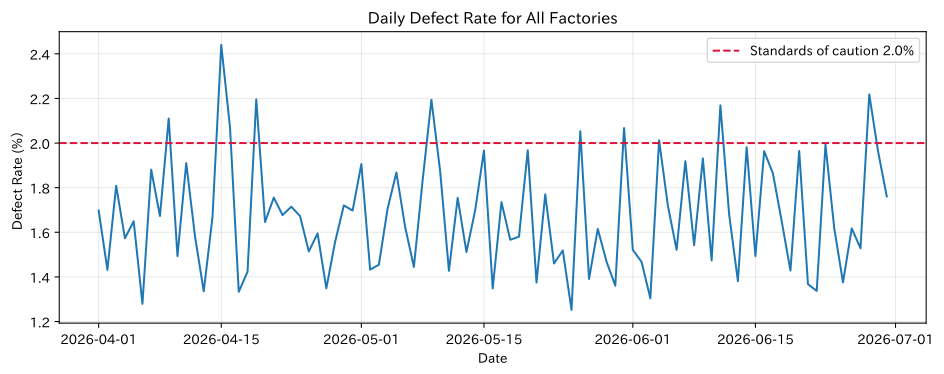
It calculates the daily number of good products, defect count, and defect rate, and returns them as series in chronological order. When compensating for days without values, you must separate “No Production” and “Data Not Arrived” to misidentify downtime and integration failures.

Check with Python

daily = (production.assign(date=production.completed_at.dt.floor("D"))
         .groupby("date", as_index=False)
         .agg(good_qty=("good_qty", "sum"), defect_qty=("defect_qty", "sum")))
daily["defect_rate_pct"] = daily.defect_qty / (daily.good_qty + daily.defect_qty) * 100
api_payload = {
    "metric": "defect_rate_pct", "unit": "%", "granularity": "day",
    "series": [{"x": d.strftime("%Y-%m-%d"), "y": round(v, 3)} for d, v in zip(daily.date.tail(5), daily.defect_rate_pct.tail(5))]
}
print(json.dumps(api_payload, ensure_ascii=False, indent=2))
fig, ax = plt.subplots(figsize=(10, 4))
ax.plot(daily.date, daily.defect_rate_pct, linewidth=1.5)
ax.axhline(2.0, color="crimson", linestyle="--", label="Standards of caution 2.0%")
ax.set_title("Daily Defect Rate for All Factories")
ax.set_xlabel("Date"); ax.set_ylabel("Defect Rate (%）")
ax.grid(True, alpha=0.3); ax.legend()
plt.tight_layout(); plt.show()

{
  "metric": "defect_rate_pct",
  "unit": "%",
  "granularity": "day",
  "series": [
    {
      "x": "2026-06-26",
      "y": 1.618
    },
    {
      "x": "2026-06-27",
      "y": 1.528
    },
    {
      "x": "2026-06-28",
      "y": 2.218
    },
    {
      "x": "2026-06-29",
      "y": 1.964
    },
    {
      "x": "2026-06-30",
      "y": 1.761
    }
  ]
}

Reading the results

Overlaying baselines over time makes it easier to distinguish between single-day deterioration and continuous deterioration. The API does not display colors or pixel coordinates, but returns dates, values, units, and missing measurements, leaving rendering responsibilities on the screen. Setting score limits and permitted granularity, and automatically aggregating weekly or monthly over long periods, is also effective.

No.088: Creating a dashboard screen

Meaning in Practice

The role of the dashboard is not to line up all the numbers, but to quickly show “where the anomaly is and what to check next.” The structure is structured so you can dig deeper into company-wide KPIs, factory comparisons, trends, and detailed notes of caution.

Approach to Analysis and Modeling

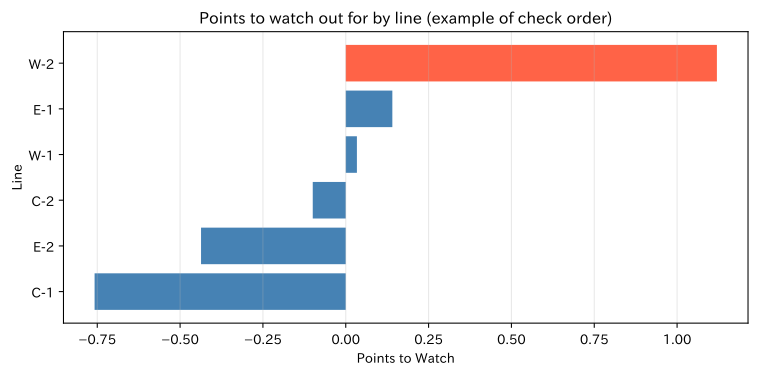
Standardize defect rates and downtime by line to create attention scores. This is not an official quality assessment, but rather an example of determining the order of inspection. In practice, define thresholds, update frequency, responsible persons, and post-click detail conditions for each KPI.

Check with Python

line_kpi = production.groupby(["factory", "line"], as_index=False).agg(
    total_qty=("total_qty", "sum"), defect_qty=("defect_qty", "sum"), downtime_min=("downtime_min", "sum"), records=("result_id", "size")
)
line_kpi["defect_rate_pct"] = line_kpi.defect_qty / line_kpi.total_qty * 100
line_kpi["downtime_per_record"] = line_kpi.downtime_min / line_kpi.records
for col in ["defect_rate_pct", "downtime_per_record"]:
    line_kpi[col + "_z"] = (line_kpi[col] - line_kpi[col].mean()) / line_kpi[col].std(ddof=0)
line_kpi["attention_score"] = 0.65 * line_kpi.defect_rate_pct_z + 0.35 * line_kpi.downtime_per_record_z
display(line_kpi.sort_values("attention_score", ascending=False).round(2))
fig, ax = plt.subplots(figsize=(8, 4))
ordered = line_kpi.sort_values("attention_score")
ax.barh(ordered.line, ordered.attention_score, color=np.where(ordered.attention_score > 0.5, "tomato", "steelblue"))
ax.set_title("Points to watch out for by line (example of check order)")
ax.set_xlabel("Points to Watch"); ax.set_ylabel("Line")
ax.grid(True, axis="x", alpha=0.3)
plt.tight_layout(); plt.show()

	factory	line	total_qty	defect_qty	downtime_min	records	defect_rate_pct	downtime_per_record	defect_rate_pct_z	downtime_per_record_z	attention_score
5	West Factory	W-2	46065	1305	3122.5	291	2.83	10.73	2.23	-0.94	1.12
2	East Factory	E-1	55605	811	4168.7	350	1.46	11.91	-0.43	1.20	0.14
4	West Factory	W-1	49784	733	3760.3	321	1.47	11.71	-0.40	0.84	0.03
1	Central Factory	C-2	35041	479	2694.0	230	1.37	11.71	-0.60	0.84	-0.10
3	East Factory	E-2	56746	838	3913.9	357	1.48	10.96	-0.39	-0.52	-0.44
0	Central Factory	C-1	40182	591	2627.5	251	1.47	10.47	-0.40	-1.42	-0.76

Reading the results

W-2 appears at the top because the defect rate is set high at the time of generation. On the dashboard, not only scores but also defect rates and downtime are displayed as evidence, and you can navigate to details filtered by relevant periods and lines. Instead of relying solely on red, it displays labels and values side by side, and always shows the last update time and data freshness.

No.089: Implementing Form and Report Output

Meaning in Practice

Reports are deliverables that share the “finalized value at that moment” during meetings, customer reports, and audits. It doesn’t just print on the screen; it records output conditions, aggregation definitions, editions, creators, and creation times. Choose Excel, CSV, and PDF according to your intended use.

Approach to Analysis and Modeling

By cross-reconciling the total of reports with the database aggregation, we provide a checksum for the number of entries, number of good products, and number of defects. Mass output is made asynchronous jobs, and measures are designed to address permissions, retention periods, personal information, and strings interpreted as formulas.

Check with Python

june = production[(production.completed_at >= "2026-06-01") & (production.completed_at < "2026-07-01")]
report = june.groupby(["factory", "line"], as_index=False).agg(
    number_of_cases=("result_id", "size"), good_quantity=("good_qty", "sum"), defective_count=("defect_qty", "sum"), stop_time=("downtime_min", "sum")
)
report["non_performing_rate_pct"] = report.defective_count / (report.good_quantity + report.defective_count) * 100
total = pd.DataFrame({
    "factory": ["All factories"], "line": ["Total"], "number_of_cases": [report.number_of_cases.sum()],
    "good_quantity": [report.good_quantity.sum()], "defective_count": [report.defective_count.sum()], "stop_time": [report.stop_time.sum()],
})
total["non_performing_rate_pct"] = total.defective_count / (total.good_quantity + total.defective_count) * 100
final_report = pd.concat([report, total], ignore_index=True)
display(final_report.round(2))
print("Match:", "OK" if total.good_quantity.iloc[0] == june.good_qty.sum() and total.defective_count.iloc[0] == june.defect_qty.sum() else "NG")
print("Ticket Requirements: 2026-06-01 00:00 <= completed_at < 2026-07-01 00:00 / version 1")

	factory	line	number_of_cases	good_quantity	defective_count	stop_time	non_performing_rate_pct
0	Central Factory	C-1	84	13353	212	876.9	1.56
1	Central Factory	C-2	73	11097	161	937.2	1.43
2	East Factory	E-1	110	17017	245	1460.8	1.42
3	East Factory	E-2	110	17571	253	1123.2	1.42
4	West Factory	W-1	108	16584	248	1274.5	1.47
5	West Factory	W-2	104	15804	447	1181.0	2.75
6	All factories	Total	589	91426	1566	6853.6	1.68

Match: OK
Form Conditions: 2026-06-01 00:00 <= completed_at < 2026-07-01 00:00 / version 1

Reading the results

The line subtotal and total for all factories match the original data. In actual reports, in addition to unit testing, the output files are reloaded to check columns, types, expressions, page breaks, and broken characters. For tasks where values change after closing, do not overwrite them; instead, add the version number and reason for correction, and allow you to reacquire past versions.

No.090: Implementing batch processing

Meaning in Practice

Daily aggregation, external collaboration, and report generation are automated in regular batches. What matters is not schedule registration, but detecting failures, safely re-reoperating, and being able to recover by the deadline.

Approach to Analysis and Modeling

Set the processing date to a unique key and re-execute on the same day to prevent double counting. The execution history records start/end, target date, number of inputs, number of outputs, status, and error summary. Not only success rate, but also pre-deadline completion rate, processing time p95, and rerun count are set as operational KPIs.

Check with Python

run_days = pd.date_range("2026-06-01", periods=30, freq="D")
duration = np.round(rng.lognormal(mean=np.log(7), sigma=0.35, size=len(run_days)), 1)
failed = rng.random(len(run_days)) < 0.10
recovered = failed & (rng.random(len(run_days)) < 0.75)
batch = pd.DataFrame({"Eligible Dates": run_days, "processing_time_minutes": duration, "first_attempt_failure": failed, "restoring_by_rerunning": recovered})
batch["final_success"] = ~batch.first_attempt_failure | batch.restoring_by_rerunning
batch["completed_before_the_deadline"] = batch.final_success & (batch.processing_time_minutes + np.where(batch.first_attempt_failure, 12, 0) <= 30)
summary = pd.Series({
    "Scheduled number of executions": len(batch), "first_time_success_rate_pct": (~batch.first_attempt_failure).mean() * 100,
    "final_success_rate_pct": batch.final_success.mean() * 100, "completion_rate_before_deadline_pct": batch.completed_before_the_deadline.mean() * 100,
    "processing_time_p95_minutes": batch.processing_time_minutes.quantile(0.95),
})
display(summary.round(1).to_frame("value"))
display(batch[batch.first_attempt_failure])

	value
Scheduled number of executions	30.0
first_time_success_rate_pct	96.7
final_success_rate_pct	100.0
completion_rate_before_deadline_pct	100.0
processing_timep95_minutes	10.4

	Eligible Dates	processing_time_minutes	first_attempt_failure	restoring_by_rerunning	final_success	completed_before_the_deadline
20	2026-06-21	8.4	True	True	True	True

Reading the results

By looking not only at the initial success rate but also at the final success rate after re-execution and the completion rate before the deadline, you can evaluate the impact on your operations. Redo decides whether to continue from the failure point or redo the entire thing, and tests double counting. Alerts not only “failed” but also notify you of the target date, process name, impact, rerun eligibility, and routing to the log.

Practical Implications Seen Through Target Exercise

1. The rules for stopping at the entrance,DBProtect by layering constraints
   Through CSV inspection, staging, unique constraints, and transactions, it gradually prevents misregistration and double registration.

2. Connecting search, aggregation, and reports to the same data definition
   By standardizing the handling of date boundaries, defect rates, and cancellation data, you can explain the numbers on screens and on forms.

3. The dashboard is designed from anomaly detection to detailed confirmation.
   It doesn’t just show KPIs—it connects to the rationale, update time, filtered details, and assigned actions.

4. Asynchronous processing is a function up to operation
   Only after re-executing the reception ID, progress, monitoring, alerts, and exponents can CSV imports and batch data be safely automated.

What is necessary for practical implementation

1. Business Definition and Data Contracts

The production, quality, and information systems departments agree on the numbering, mandatory items, units, shift boundaries, closure, correction, cancellation, and KPI calculation formulas for the performance ID. The CSV and API specifications are managed as versions, and a transition period is set for changes in the event of change.

2. Performance and Capacity Design

It measures the number of entries during normal and closing times, file size, retention period, concurrent users, and allowable response times, and designs indexes, page sizes, caches, and asynchronization. You cannot use the results of fictitious data directly for performance assurance.

3. Security and Auditing

We organize permissions by factory and job role, inspection of uploaded files, measures against SQL injection, report retention deadlines, and history, operation, correction, and output history. It is also important not to publish sensitive information in logs or error messages.

4. Testing and operational KPIs

Tests boundary dates, 0 cases, large capacity, duplicates, partial failures, reruns, and post-tightening corrections. In production, we monitor import success rate, search page 95, data freshness, pre-deadline completion rate, and reconciliation variance, and establish recovery procedures with the person in charge.

Conclusion

From No.081 to No.090, we confirmed the flow of safely registering manufacturing results received via CSV into a database, expanding them into lists, searches, aggregations, graphs, dashboards, and reports, and continuing batch operations.

The key is not to think of each function as a standalone screen or API, but to connect them with the same data definitions, point in time, and audit trail. By designing not only normal systems but also overlaps, boundaries, delays, failures, and reruns, business systems become the “data storage box” and the foundation for the field to make evidence-based decisions.

Consultations for Corporations

At Suri Kobo, we provide comprehensive support for everything from organizing CSV and Excel operations in manufacturing, designing and developing data infrastructure and business systems, defining KPIs, dashboards, and managing forms and batches.

• I want to consolidate different achievement files for each factory.
• Want to match the numbers on screens, meeting materials, and forms
• Want to speed up searching and aggregating large volumes of data
• Want to safely automate manual aggregation and report creation
• Want to integrate AI and optimization model results into existing operations

Even before your requirements are finalized, you can consult us starting with inventory of current operations and data.

📩 Contact Us: surikobo.co.jp/contact
Please feel free to consult us first.