Making AI a ‘usable system’ in manufacturing — Prediction, anomaly detection, optimization, and 10 exercise-on LLM implementations

Focusing on production planning, equipment maintenance, and quality management on the manufacturing floor, we will continuously organize everything from API implementation of machine learning models, demand forecasting, anomaly detection, dashboards, optimization results, LLM utilization, operations design, to overall architecture. This article focuses not only on creating highly accurate models but also on designing them up to the Who looks at what grounds, when, and which actions to choose?.

[!NOTE] This material is a notebook previously used by Surikoubo (or personally by the representative, Kazuyama), and has been reconstructed, edited, and published with the company’s permission.
All data listed is fictional and has no relation whatsoever to real companies, factories, or figures.

Introduction: Practical Challenges in Manufacturing Covered in This Article

When advancing AI utilization in manufacturing, they face challenges such as predictive models that were good in PoCs being not referenced on site, too many abnormal alerts that are ignored, and planners unable to adopt the optimization results due to unclear reasons. The cause is not just model accuracy. The fact that input data freshness, API responses, on-screen explanations, approval permissions, alternative procedures in case of failures, and monitoring for model degradation are not designed as a single business system has a major impact.

This paper assumes a fictional precision parts factory and generates monthly demand, equipment sensors, line capabilities, and AI service operation logs. Forecast values and anomaly scores are linked to concrete decisions such as order volume, maintenance inspections, and daily production planning.

Common situations on site

• Only the predicted values are displayed, and the forecast range and assumptions are unknown.
• Unable to explain the reason for the high abnormal score to the maintenance staff
• If the AI API stops, you will no longer be able to use the work instruction screen.
• Unable to verify whether the recommended plan meets constraints such as equipment capacity, scheduling, or inventory
• Confidential or personal information is sent directly to LLMs
• Even if accuracy deteriorates after model updates, no one notices
• Recruitment and rejection by the field are not recorded, and the reasons behind them are not recorded, leading to no improvement.

Why is this issue so difficult to judge?

There is uncertainty in AI output. If demand forecasts are shown only as point forecasts $\hat{y}_{t+h}$, it is impossible to assess the impact of forecast errors on decision-making. In practice, it is indicated along with the lower limit $L_{t+h}$ and upper limit $U_{t+h}$, which leads to safety stock and overtime assessments.

Additionally, anomaly detection involves trade-offs between false positives and missed detections. Lowering the threshold increases the recall rate, but also increases the number of inspections. The optimal threshold is determined not only by model metrics but also by missed losses, inspection man-hours, and equipment downtime risk. Furthermore, if any one of AI, APIs, screens, or business procedures is missing, the on-site decision-making process is incomplete.

Overview of Exercise covered this time

No.	Theme	Practical Points to Check
091	API Implementation of Machine Learning Models	I/O contracts, block management, response performance
092	Demand Forecasting API	Forecast Sections and Order Decisions
093	Anomaly Detection API	Thresholds, false alarms, missed spots
094	Forecast dashboard	Exception-focused comparison display
095	Abnormal alert screen	Priority and Response Deadlines
096	Displaying optimization results	Constraints, Rationales, and Acceptance or Rejection Records
097	Summarizing tasks with LLMs	Evidence, confidentiality, and confirmation of people
098	Chat Inquiries	Intent, Permissions, and Audit Logs
099	Model, API, and Screen Operations	SLO, drift, and rewinding
100	AI-Utilizing System Design	From Challenges to KPIs, Structure, and Implementation Plans

Preparing the Python environment

Generate and aggregate fictional data using numpy and pandas, and visualize it in matplotlib. Japanese is displayed using japanize_matplotlib. It does not connect to external data or external AI APIs. Fix the random number seed so you can reproduce the same result.

%matplotlib inline
%config InlineBackend.figure_format = 'svg'

import sys
import numpy as np
import pandas as pd
import matplotlib
import matplotlib.pyplot as plt
import japanize_matplotlib

rng = np.random.default_rng(20260712)
pd.set_option("display.max_columns", 20)
pd.set_option("display.width", 140)

print(f"Python     : {sys.version.split()[0]}")
print(f"numpy      : {np.__version__}")
print(f"pandas     : {pd.__version__}")
print(f"matplotlib : {matplotlib.__version__}")

Python     : 3.13.1
numpy      : 2.5.1
pandas     : 3.0.3
matplotlib : 3.11.0

Creation of Fictional Data

It generates 156 weeks of weekly demand for three products, 1,200 sensor records from six devices, next-week planning candidates for three lines, and 2,000 AI API operation logs. Demand includes seasonality and promotional effects, while sensors include temperature and vibration increases associated with deterioration. The following data are for explanatory purposes and are fictitious and do not indicate actual measurement accuracy.

weeks = pd.date_range("2023-07-03", periods=156, freq="W-MON")
products = ["precision gearA", "precision gearB", "drive shaftC"]
rows = []
for p, base, amp in zip(products, [520, 390, 300], [75, 45, 35]):
    for i, week in enumerate(weeks):
        promo = int(i % 26 in [4, 5])
        demand = base + amp * np.sin(2 * np.pi * i / 52) + 65 * promo + rng.normal(0, 32)
        rows.append([week, p, promo, max(0, round(demand))])
demand = pd.DataFrame(rows, columns=["week", "product", "promotion", "actual_qty"])

n_sensor = 1200
sensors = pd.DataFrame({
    "timestamp": pd.date_range("2026-06-01", periods=n_sensor, freq="15min"),
    "machine": rng.choice([f"MC-{i:02d}" for i in range(1, 7)], n_sensor),
    "load_pct": rng.uniform(45, 98, n_sensor),
})
sensors["degradation"] = np.clip(np.arange(n_sensor) / n_sensor + rng.normal(0, .08, n_sensor), 0, 1)
sensors["temperature_c"] = 48 + .16*sensors["load_pct"] + 9*sensors["degradation"] + rng.normal(0, 2, n_sensor)
sensors["vibration_mm_s"] = 1.1 + .012*sensors["load_pct"] + 2.1*sensors["degradation"] + rng.normal(0, .25, n_sensor)
sensors["true_anomaly"] = (sensors["temperature_c"] > 69) | (sensors["vibration_mm_s"] > 3.8)

api_logs = pd.DataFrame({
    "service": rng.choice(["Demand forecasting", "anomaly detection", "Optimization"], 2000, p=[.45, .4, .15]),
    "model_version": rng.choice(["v2.3", "v2.4"], 2000, p=[.35, .65]),
    "latency_ms": np.round(rng.lognormal(5.35, .48, 2000)),
    "success": rng.random(2000) > .018,
    "input_missing": rng.random(2000) < .025,
})

print("Demand Data:", demand.shape, "Equipment Sensor Data:", sensors.shape, "APILog:", api_logs.shape)
display(demand.tail(6), sensors.head(5))

Demand data: (468, 4) Equipment sensor data: (1200, 7) API log: (2000, 5)

	week	product	promotion	actual_qty
462	2026-05-18	drive shaftC	0	324
463	2026-05-25	drive shaftC	0	249
464	2026-06-01	drive shaftC	0	375
465	2026-06-08	drive shaftC	0	277
466	2026-06-15	drive shaftC	0	245
467	2026-06-22	drive shaftC	0	274

	timestamp	machine	load_pct	degradation	temperature_c	vibration_mm_s	true_anomaly
0	2026-06-01 00:00:00	MC-01	94.184648	0.019594	65.098978	2.324577	False
1	2026-06-01 00:15:00	MC-06	83.966129	0.000000	60.966094	2.301255	False
2	2026-06-01 00:30:00	MC-02	97.884000	0.134691	64.597830	2.489244	False
3	2026-06-01 00:45:00	MC-01	77.891433	0.079755	59.151385	2.118854	False
4	2026-06-01 01:00:00	MC-01	49.893098	0.062595	57.250918	1.531000	False

No.091: API the Machine Learning Model

Meaning in Practice

By API-based models, you can use the same inference functions from the production management screen, maintenance screen, and batch processing. However, simply loading a trained model and returning numbers is not enough. Contracts are defined as input items, units, handling of missing items, model versions, inference times, and error formats.

Approach to Analysis and Modeling

We check API operational quality as percentiles of success rate and response time. The 95th percentile is the boundary where 95% of calls are completed within that timeframe. Averages alone overlook some extremely slow responses. The basic design is to load the model at startup and avoid reloading for each request.

Check with Python

api_summary = (api_logs.groupby("service")
    .agg(number_of_outflows=("success", "size"), success_rate_pct=("success", "mean"),
         median_ms=("latency_ms", "median"),
         p95_ms=("latency_ms", lambda x: x.quantile(.95)),
         input_missing_rate_pct=("input_missing", "mean")))
api_summary[["success_rate_pct", "input_missing_rate_pct"]] *= 100
display(api_summary.round(1))

sample_response = {"prediction": 548, "unit": "units/week", "model_version": "v2.4",
                   "predicted_at": "2026-07-12T09:00:00+09:00", "request_id": "REQ-091-001"}
sample_response

	number_of_outflows	success_rate_pct	median_ms	p95_ms	input_missing_rate_pct
service
Optimization	277	98.6	203.0	431.4	3.6
anomaly detection	821	98.7	220.0	486.0	2.9
Demand forecasting	902	97.3	205.5	475.3	2.2

{'prediction': 548,
 'unit': 'units/week',
 'model_version': 'v2.4',
 'predicted_at': '2026-07-12T09:00:00+09:00',
 'request_id': 'REQ-091-001'}

Reading the results

By dividing success rates and p95 by service, you can determine screen timeout values and prioritize performance improvements. Responses include not only the forecast value but also units, model versions, times, and the request ID used for inquiries. In production, authentication, input schema validation, maximum number of entries, idempotence, and audit logs are also defined, and in case of failure, you can switch to the previous confirmed value or manual calculation.

No.092: Creating a Demand Forecasting API

Meaning in Practice

The demand forecasting API receives products and forecast periods, and returns future demand. What users need is not a single forecast value, but rather the basis for ordering and capacity adjustment decisions based on that range.

Approach to Analysis and Modeling

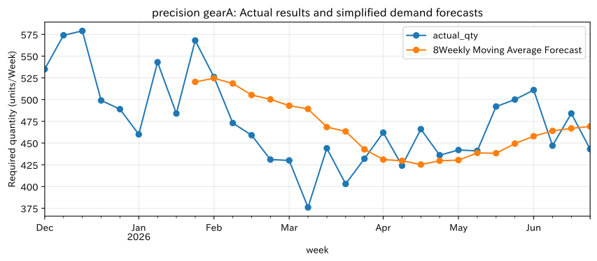
Here, we use a simplified forecast that multiplies the most recent 8-week average by the seasonal index. As an example to simplify explanations, in practice, candidate models are compared using time series cross-validation. Prediction error is mean absolute error

$MAE=\frac{1}{n}\sum_{i=1}^{n}|y_i-\hat{y}_i|$

and create an approximately 80% predicted interval based on the standard deviation of the most recent residual.

Check with Python

forecast_rows = []
for product in products:
    d = demand[demand["product"] == product].copy()
    d["forecast"] = d["actual_qty"].shift(1).rolling(8).mean()
    valid = d.dropna(subset=["forecast"])
    sigma = (valid["actual_qty"] - valid["forecast"]).tail(52).std()
    next_point = d["actual_qty"].tail(8).mean()
    forecast_rows.append([product, round(next_point), round(next_point-1.28*sigma),
                          round(next_point+1.28*sigma), round(np.mean(abs(valid["actual_qty"]-valid["forecast"])), 1)])
forecast = pd.DataFrame(forecast_rows, columns=["product", "forecast_qty", "lower_80", "upper_80", "backtest_MAE"])
display(forecast)

plot_d = demand[demand["product"] == "precision gearA"].tail(30).copy()
plot_d["8Weekly Moving Average Forecast"] = plot_d["actual_qty"].shift(1).rolling(8).mean()
ax = plot_d.plot(x="week", y=["actual_qty", "8Weekly Moving Average Forecast"], figsize=(9, 4), marker="o")
ax.set_title("precision gearA: Actual results and simplified demand forecasts")
ax.set_xlabel("week")
ax.set_ylabel("Required quantity (units/Week)")
ax.grid(True, alpha=.3)
plt.tight_layout()
plt.show()

	product	forecast_qty	lower_80	upper_80	backtest_MAE
0	precision gearA	470	407	533	36.3
1	precision gearB	380	334	425	32.5
2	drive shaftC	283	232	334	30.7

Reading the results

The upper limit of the forecast range can be used to check capacity and materials when avoiding stockouts is important, while the lower limit is used to check for the risk of excess inventory. The API also returns the forecast period, forecast creation time, last day of data used, and the confidence level of the segment. Since MAE depends on the quantity scale of the product, product comparisons often use indicators such as dividing MAE by average demand, as well as asymmetric costs from out-of-stock or surplus.

No.093: Creating an Anomaly Detection API

Meaning in Practice

The anomaly detection API receives sensor values and returns the degree of anomaly and the reason for the judgment. The goal is not to increase alerts, but to narrow down inspection targets before failures occur.

Approach to Analysis and Modeling

Temperature and vibration are standardized, and a score combining positive deviations is used. Compare the accuracy $Precision=TP/(TP+FP)$, recall $Recall=TP/(TP+FN)$, and number of alerts for each threshold. For equipment with high missed rates, reproduction is prioritized, and when inspection capabilities are limited, a balance is maintained with the accuracy rate.

Check with Python

for col in ["temperature_c", "vibration_mm_s"]:
    sensors[f"z_{col}"] = (sensors[col] - sensors[col].mean()) / sensors[col].std()
sensors["anomaly_score"] = np.sqrt(np.maximum(sensors["z_temperature_c"], 0)**2 +
                                    np.maximum(sensors["z_vibration_mm_s"], 0)**2)

metrics = []
for threshold in [1.0, 1.5, 2.0, 2.5]:
    pred = sensors["anomaly_score"] >= threshold
    truth = sensors["true_anomaly"]
    tp, fp, fn = (pred & truth).sum(), (pred & ~truth).sum(), (~pred & truth).sum()
    metrics.append([threshold, pred.sum(), tp/(tp+fp) if tp+fp else 0, tp/(tp+fn) if tp+fn else 0, fn])
thresholds = pd.DataFrame(metrics, columns=["threshold", "Number of alerts", "Compatibility rate", "recall rate", "Number of missed cases"])
display(thresholds.round(3))

	threshold	Number of alerts	Compatibility rate	recall rate	Number of missed cases
0	1.0	351	0.735	1.000	0
1	1.5	200	0.995	0.771	59
2	2.0	80	1.000	0.310	178
3	2.5	31	1.000	0.120	227

Reading the results

Raising the threshold reduces the number of alerts but may increase missed incidents. Therefore, instead of deciding solely on the model manager that “a score of 2 or higher means abnormality,” the maintenance team checks the loss of one missed case, the man-hours required for one inspection, and the number of cases that can be handled daily. The API returns judgments, scores, thresholds, and key contributing items, and notifies sensor defects or values outside the learning range separately from regular judgments.

No.094: Displaying Forecast Results on the Dashboard

Meaning in Practice

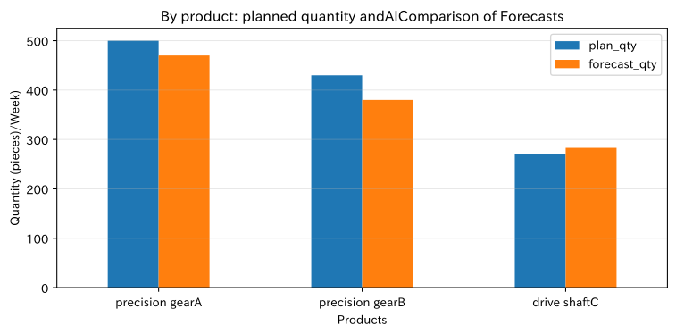
The purpose of the dashboard is not to list all forecasts, but to quickly identify products where there is a significant gap between planning and AI predictions and that require action.

Approach to Analysis and Modeling

Compare sales and production plans with forecasts to create difference rates and out-of-forecast criteria. The difference rate is

$Gap(\%)=\frac{Forecast-Plan}{Plan}\times100$

If the absolute difference is 10% or more, or if the plan is outside the 80% forecast range, confirmation is required.

Check with Python

dashboard = forecast.copy()
dashboard["plan_qty"] = [500, 430, 270]
dashboard["gap_pct"] = 100 * (dashboard["forecast_qty"] - dashboard["plan_qty"]) / dashboard["plan_qty"]
dashboard["outside_interval"] = ((dashboard["plan_qty"] < dashboard["lower_80"]) |
                                 (dashboard["plan_qty"] > dashboard["upper_80"]))
dashboard["status"] = np.where((dashboard["gap_pct"].abs() >= 10) | dashboard["outside_interval"], "Needs confirmation", "within the range")
display(dashboard[["product", "plan_qty", "forecast_qty", "lower_80", "upper_80", "gap_pct", "status"]].round(1))

ax = dashboard.plot.bar(x="product", y=["plan_qty", "forecast_qty"], figsize=(8, 4), rot=0)
ax.set_title("By product: planned quantity andAIComparison of Forecasts")
ax.set_xlabel("Products")
ax.set_ylabel("Quantity (pieces)/Week)")
ax.grid(True, axis="y", alpha=.3)
plt.tight_layout()
plt.show()

	product	plan_qty	forecast_qty	lower_80	upper_80	gap_pct	status
0	precision gearA	500	470	407	533	-6.0	within the range
1	precision gearB	430	380	334	425	-11.6	Needs confirmation
2	drive shaftC	270	283	232	334	4.8	within the range

Reading the results

Display products with large differences at the front, linking to next steps such as plan changes, material confirmation, or sales confirmation. The graph displays not only plans and forecasts, but also forecast intervals, actual performance trends, and the time of the last data update. Rather than relying solely on red, we will design it so that both “Confirmation Needed” and reasons are written, allowing users to record the reasons for adopting or rejecting predictions.

No.095: Creating an Abnormal Alert Screen

Meaning in Practice

The alert screen is not a list of abnormalities, but rather a workbench where a limited number of maintenance personnel decide the order of response. Equipment, occurrence time, reason for abnormalities, impact, confirmation deadline, responsible person, and response status are all connected on a single screen.

Approach to Analysis and Modeling

Priority is calculated by combining anomaly scores, equipment importance, and unconfirmed time. Scores are used as an aid for prioritization and must not override forced stops based on safety standards. Similar alerts are bundled together for a set period, reducing notification fatigue.

Check with Python

alerts = sensors[sensors["anomaly_score"] >= 1.5].copy()
importance = {"MC-01": 3, "MC-02": 2, "MC-03": 3, "MC-04": 1, "MC-05": 2, "MC-06": 1}
alerts["Equipment Importance"] = alerts["machine"].map(importance)
alerts["unconfirmed_time_min"] = rng.integers(0, 91, len(alerts))
alerts["Priority score"] = alerts["anomaly_score"]*2 + alerts["Equipment Importance"] + alerts["unconfirmed_time_min"]/30
alerts["main reason"] = np.where(alerts["z_temperature_c"] >= alerts["z_vibration_mm_s"], "temperature rise", "Vibration rise")
alert_view = alerts.nlargest(10, "Priority score")[["timestamp", "machine", "main reason", "anomaly_score", "Equipment Importance", "unconfirmed_time_min", "Priority score"]]
display(alert_view.round(2))

/var/folders/3y/fmw40k0x78xblvb3gkcyvy1h0000gn/T/ipykernel_48148/2855950023.py:8: UserWarning: obj.round has no effect with datetime, timedelta, or period dtypes. Use obj.dt.round(...) instead.
  display(alert_view.round(2))

	timestamp	machine	main reason	anomaly_score	Equipment Importance	unconfirmed_time_min	Priority score
1173	2026-06-13 05:15:00	MC-01	temperature rise	3.28	3	57	11.45
1106	2026-06-12 12:30:00	MC-03	temperature rise	2.57	3	88	11.07
1030	2026-06-11 17:30:00	MC-03	Vibration rise	2.88	3	68	11.03
929	2026-06-10 16:15:00	MC-01	temperature rise	2.57	3	83	10.90
1113	2026-06-12 14:15:00	MC-03	temperature rise	2.60	3	71	10.56
1169	2026-06-13 04:15:00	MC-01	temperature rise	3.34	3	26	10.56
1196	2026-06-13 11:00:00	MC-05	temperature rise	2.78	2	89	10.52
1157	2026-06-13 01:15:00	MC-01	Vibration rise	2.31	3	85	10.45
832	2026-06-09 16:00:00	MC-05	temperature rise	2.86	2	79	10.35
1161	2026-06-13 02:15:00	MC-02	Vibration rise	2.99	2	70	10.31

Reading the results

By including not only the degree of abnormality but also the importance of equipment and elapsed time, you can create a response order that reflects the impact on the business. On the screen, “Confirmation,” “Inspection Instructions,” “False Reports,” and “Pending” are recorded, and critical alerts are notified in stages until the person in charge receives them. False reports can be used to improve the model, but if directly linked to on-site evaluation indicators, input becomes distorted, so clearly share the purpose of improvement.

No.096: Displaying the results of optimization calculations on the screen

Meaning in Practice

The results of production optimization cannot be adopted by quantity alone. You need to explain what is improving over current plans, as well as meeting constraints such as capacity, inventory, delivery time, and scheduling.

Approach to Analysis and Modeling

As a simplified allocation problem, the production volume $x_p$ of product $p$ is assigned in order of highest profit up to the demand ceiling. The purpose is

$\max \sum_p m_p x_p,\quad \mathrm{s.t.}\ \sum_p a_p x_p\le C,\ 0\le x_p\le d_p$

That’s right. Here, $m_p$ is marginal profit, $a_p$ is the labor per task, and $C$ is total capacity.

Check with Python

plan = pd.DataFrame({"product": products, "demand": forecast["forecast_qty"],
                     "margin_yen": [1300, 1050, 1600], "minutes_per_unit": [2.4, 1.8, 3.2]})
capacity = 2450
plan["interest/minutes"] = plan["margin_yen"] / plan["minutes_per_unit"]
remaining = capacity
qty = []
for i in plan.sort_values("interest/minutes", ascending=False).index:
    q = min(plan.loc[i, "demand"], int(remaining // plan.loc[i, "minutes_per_unit"]))
    qty.append((i, q)); remaining -= q * plan.loc[i, "minutes_per_unit"]
plan["Recommended production volume"] = 0
for i, q in qty: plan.loc[i, "Recommended production volume"] = q
plan["insufficient amount"] = plan["demand"] - plan["Recommended production volume"]
plan["usage_min"] = plan["Recommended production volume"] * plan["minutes_per_unit"]
display(plan.round(1))
print(f"Ability usage: {plan['usage_min'].sum():,.1f}/{capacity:,}Points, residual capacity: {remaining:,.1f}minutes")

	product	demand	margin_yen	minutes_per_unit	interest/minutes	Recommended production volume	insufficient amount	usage_min
0	precision gearA	470	1300	2.4	541.7	470	0	1128.0
1	precision gearB	380	1050	1.8	583.3	380	0	684.0
2	drive shaftC	283	1600	3.2	500.0	199	84	636.8

Ability Usage: 2,448.8/2,450 points, Residual Ability: 1.2 points

Reading the results

The screen displays recommended quantities, capacity usage, shortage amounts, objective functions, and key constraints. If the person in charge overwrites the quantity, the constraint is recalculated and the violation is indicated on the spot. This example simplifies continuous capability allocation. In practice, integer optimization is required, including lots, setup sequences, equipment fit, materials, personnel, and maintenance schedules, and not only optimal solutions but also feasible alternatives are useful.

No.097: Summarizing Business Data with LLMs

Meaning in Practice

LLMs can quickly create drafts for daily reports and meeting materials. On the other hand, since numerical errors or unfounded explanations may be mixed in, it is safer to finalize aggregation using Python or SQL and to assign LLMs to document the finalized values.

Approach to Analysis and Modeling

Separate “Search & Aggregation” from “Text Generation.” Inputs should include target periods, KPIs, comparison criteria, and basis record IDs, while outputs should be structured as summaries, candidate factors, and recommended confirmations. Personal names and business partner names are kept secret before sending, and only after approval are distributed by the user.

Check with Python

facts = {
    "Eligible Period": "2026-06-01〜2026-06-13",
    "Number of sensors": len(sensors),
    "value_value": int(sensors["true_anomaly"].sum()),
    "threshold1.5Number of alerts": int((sensors["anomaly_score"] >= 1.5).sum()),
    "Highest Score Facilities": sensors.loc[sensors["anomaly_score"].idxmax(), "machine"],
    "Highest Anomaly Score": round(sensors["anomaly_score"].max(), 2),
}
prompt_template = (
    "You are the record supporter for equipment maintenance meetings.\n"
    "The following have been confirmedJSONBased solely on this, summarize the facts, points to be verified, and the following actions in Japanese.\n"
    "Do not make definitive conclusions about unfounded causes; please add units to the numbers.\n"
    f"Input: {facts}"
)
print(prompt_template)

You are the record supporter for equipment maintenance meetings.
Based only on the confirmed JSON, summarize in Japanese the facts, points to be verified, and next actions.
Do not make definitive conclusions about unfounded causes; please add units to the numbers.
Input: {'Target period': '2026-06-01–2026-06-13', 'Number of sensors': 1200, 'True anomaly count_for verification': 258, 'Number of alerts with threshold 1.5': 200, 'Highest score equipment': 'MC-01', 'Highest anomaly score': np.float64(3.34)}

Reading the results

Instead of letting LLMs freely search for data, they provide confirmed facts and explicit instructions, which helps suppress numerical errors and excessive assertions. Generate text with links to the source data, generation time, model information, and unconfirmed markings. Quality is evaluated not only by fluency of writing but also by numerical consistency rate, evidence presentation rate, revision rate, and approval time. This notebook does not call external LLMs.

No.098: Querying Business Data via Chat

Meaning in Practice

With a chat format, users can ask questions in business terms, such as “Which equipment should be prioritized for inspection this week?” However, searching for vague periods or data beyond your permission can lead to plausible incorrect answers or information leaks.

Approach to Analysis and Modeling

Convert questions into intent, target, duration, and metrics, and assign them to authorized search templates. Instead of directly generating and executing SQL freely, it applies read-only views, row-level permissions, and count limits. Return the conditions you have implemented and the number of supporting documents for your response.

Check with Python

questions = pd.DataFrame({
    "Question": ["Show this week's demand forecast by product", "Which equipment has the most abnormalities?", "Please tell me your evaluation of Mr. Tanaka.", "What is the optimal production volume for next month?"],
    "Intention": ["forecast", "anomaly_rank", "personnel", "optimization"],
    "Required Permissions": ["View Production Plan", "Conservation Viewing", "personnel confidentiality", "Production Plan Edit"],
    "User rights available": [True, True, False, True],
    "Clear period": [True, False, True, True],
})
questions["Judgment"] = np.select(
    [~questions["User rights available"], ~questions["Clear period"]],
    ["Denial: Lack of authority", "Confirmation: Specify the period"], default="executable")
display(questions)

	Question	Intention	Required Permissions	User rights available	Clear period	Judgment
0	Show this week's demand forecast by product	forecast	View Production Plan	True	True	executable
1	Which equipment has the most abnormalities?	anomaly_rank	Conservation Viewing	True	False	Confirmation: Specify the period
2	Please tell me your evaluation of Mr. Tanaka.	personnel	personnel confidentiality	False	True	Denial: Lack of authority
3	What is the optimal production volume for next month?	optimization	Production Plan Edit	True	True	executable

Reading the results

For questions about insufficient permissions, reject them before generating an answer, and if the period is unclear, confirm with “Is the last 7 days acceptable?” The response screen displays the target period, filters, aggregation time, and number of references, allowing users to navigate to the original data. Questions, converted search terms, execution results, answers, and user evaluations are recorded in the audit log, but unnecessary personal information is not stored.

No.099: Organizing the operational design of models, APIs, and screens

Meaning in Practice

After the AI system is published, its data distribution, equipment, product types, and operational rules will change. If you monitor models, APIs, and screens separately, users may be struggling while each person’s metrics remain normal.

Approach to Analysis and Modeling

KPIs and responsible persons are defined at three levels: model quality, service quality, and business outcomes. As a simple example of data drift, check the standardized mean deviation obtained by dividing the average temperature difference between the reference period and the most recent period by the reference standard deviation. Exceeding the threshold is not automatic relearning, but rather a signal to start the investigation.

Check with Python

baseline = sensors.iloc[:400]
recent = sensors.iloc[-400:]
drift = (recent["temperature_c"].mean() - baseline["temperature_c"].mean()) / baseline["temperature_c"].std()
ops = pd.DataFrame({
    "layer": ["Model", "Model", "API", "API", "Screens & Operations", "Screens & Operations"],
    "indicator": ["Demand forecastingMAE", "temperature drift", "success_rate", "p95_response_time", "Recommended Adoption Rate", "Alert Confirmation Time"],
    "present value": [forecast["backtest_MAE"].mean(), drift,
              100*api_logs["success"].mean(), api_logs["latency_ms"].quantile(.95), 68.0, 14.0],
    "Monitoring standards": ["Product-specific standard ratio+20%", "|value| >= 0.5", ">= 99.0%", "<= 800ms", "Monitoring by Reason", "<= 15minutes"],
    "primary responsible person": ["Analysis Specialist", "Analysis Specialist", "System Staff", "System Staff", "Production management", "Person responsible for preservation"],
})
display(ops.round(2))

	layer	indicator	present value	Monitoring standards	primary responsible person
0	Model	Demand forecastingMAE	33.17	Product-specific standard ratio+20%	Analysis Specialist
1	Model	temperature drift	1.96	|value| >= 0.5	Analysis Specialist
2	API	success_rate	98.05	>= 99.0%	System Staff
3	API	p95response time	476.00	<= 800ms	System Staff
4	Screens & Operations	Recommended Adoption Rate	68.00	Monitoring by Reason	Production management
5	Screens & Operations	Alert Confirmation Time	14.00	<= 15minutes	Person responsible for preservation

Reading the results

If the standardized mean deviation exceeds the standard, investigations are conducted on sensor calibration, load configuration, season, and equipment degradation. We record both model and data versions, compare the old and new versions with minimal impact, and then deploy them. We also practice in advance on degenerate operation during API failures, switching back to the old version, communication networks, and decision deadlines. Retraining is conducted only after approving not only accuracy but also fairness, safety, and alignment with business rules.

No.100: Designing AI utilization systems from business challenges

Meaning in Practice

Finally, we conceive from business challenges rather than technical aspects. Rather than “introducing AI,” define target judgment and expected outcomes by “reducing plan changes due to material shortages” or “early detection of sudden outages.”

Approach to Analysis and Modeling

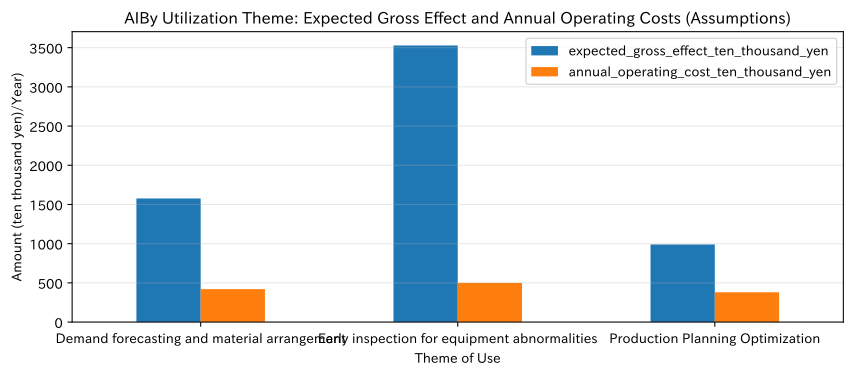
Issues and users, decision-making, input, AI output, behavior, KPIs, and response to failure are all compiled into a single causal hypothesis. The effectiveness of implementation is estimated based on the number of cases targeted× current losses × improvement rate, and compared to development and operational costs. Even if AI accuracy is high, low usage rates will not yield results, so business effectiveness is broken down as follows.

$Expected\ Benefit = Opportunities \times Adoption\ Rate \times Correct\ Action\ Rate \times Value\ per\ Action$

Check with Python

scenarios = pd.DataFrame({
    "Theme of Use": ["Demand forecasting and material arrangement", "Early inspection for equipment abnormalities", "Production Planning Optimization"],
    "Annual Judgment Opportunities": [156, 240, 52],
    "Adoption rate": [.72, .60, .80],
    "Correct Behavior Rate": [.78, .70, .85],
    "value_1_action_value_ten_thousand_yen": [18, 35, 28],
    "annual_operating_cost_ten_thousand_yen": [420, 500, 380],
})
scenarios["expected_gross_effect_ten_thousand_yen"] = (scenarios["Annual Judgment Opportunities"] * scenarios["Adoption rate"] *
                              scenarios["Correct Behavior Rate"] * scenarios["value_1_action_value_ten_thousand_yen"])
scenarios["after_operating_expenses_deducted_ten_thousand_yen"] = scenarios["expected_gross_effect_ten_thousand_yen"] - scenarios["annual_operating_cost_ten_thousand_yen"]
display(scenarios.round(1))

ax = scenarios.plot.bar(x="Theme of Use", y=["expected_gross_effect_ten_thousand_yen", "annual_operating_cost_ten_thousand_yen"], figsize=(9, 4), rot=0)
ax.set_title("AIBy Utilization Theme: Expected Gross Effect and Annual Operating Costs (Assumptions)")
ax.set_xlabel("Theme of Use")
ax.set_ylabel("Amount (ten thousand yen)/Year)")
ax.grid(True, axis="y", alpha=.3)
plt.tight_layout()
plt.show()

	Theme of Use	Annual Judgment Opportunities	Adoption rate	Correct Behavior Rate	1The value of action_ten_thousand_yen	annual_operating_cost_ten_thousand_yen	expected_gross_effect_ten_thousand_yen	after_operating_expenses_deducted_ten_thousand_yen
0	Demand forecasting and material arrangement	156	0.7	0.8	18	420	1577.0	1157.0
1	Early inspection for equipment abnormalities	240	0.6	0.7	35	500	3528.0	3028.0
2	Production Planning Optimization	52	0.8	0.8	28	380	990.1	610.1

Reading the results

Estimates rely heavily on assumptions and are not a definitive value of investment effectiveness. However, when you specify adoption rates, it becomes clear that not only improving model accuracy but also enhancing explanations, education, and operational procedures will determine value. First, we measure current KPIs on a one-line-per-judgment basis, conduct trials with manual approval, confirm safety and effectiveness, and then expand the scope. Rule-based systems without AI or when business improvements are appropriate are also included as comparison options.

Practical Implications Seen Through Target Exercise

1. AIMaking decision-making the design unit rather than the output
   First, we define how predictions, anomaly scores, and optimal solutions lead to confirmation, approval, and action by the person in charge.
2. Leaving uncertainty and evidence on screen
   Prediction intervals, reasons for judgment, constraints, data timepoints, and model versions help suppress both user overconfidence and distrust.
3. Model metrics and operationsKPIto separate and tie
   We track not only MAE and reproduction rate, but also outages, stoppages, inspection man-hours, adoption rates, and confirmation times.
4. Designing failures as normal
   We provide degenerate operation and human verification for defects, out-of-range inputs, API outages, false positives, and LLM misgeneration.
5. Returning operational data to the next improvement
   Reasons for acceptance or rejection, reasons for false reports, inquiries, and edition information are recorded in an auditable form and used for retraining and screen improvement.

What is necessary for practical implementation

1. Definition of Separation of Work and Responsibility

Define the target decisions, deadlines, approvers, the scope of AI proposals, and the conditions that must be checked by humans. We prioritize laws and regulations related to safety and quality, internal standards, and customer requirements.

2. Data and Security

Determine data owners, quality standards, update frequency, retention period, and access permissions. When using LLMs, we verify the data that can be transmitted, contractual learning use, storage destinations, and confidential information.

3. Non-functional requirements for API, screen, and operation

Define availability, response time, peak count, audit logs, backups, rollbacks, and outage procedures. Enable tracking of model versions, feature versions, inputs, and outputs.

4. Phased Implementation and Effectiveness Verification

We measure current values and reduce risk in the order of historical data verification, shadow operations, limited use, and phased rollout. Regular reviews of accuracy, operational performance, utilization, and safety are conducted, and stoppage standards are also established.

Conclusion

From No.091 to No.100, we reviewed everything from API implementation of machine learning models, demand forecasting, anomaly detection, dashboards, alerts, optimization, LLMs, chat inquiries, operational design, to the overall concept of an AI-utilizing system.

The key to turning AI into value in manufacturing is not the competition in the accuracy of individual models. It is designed as a decision-making system that includes input data quality, uncertainty display, on-site approval, substitution in case of failures, and continuous monitoring. Simulations made with hypothetical data are used as a starting point to verify field data and operational constraints.

Consultations for Corporations

At Suri Kobo, we provide comprehensive support for everything from business organization in manufacturing industries, data analysis, demand forecasting, anomaly detection, mathematical optimization, and LLM model development, to implementation on APIs, business dashboards, and monitoring platforms.

• I want to select AI utilization themes and organize investment returns.
• Want to integrate the PoC model into the on-site system
• Want a screen that can explain prediction, anomaly, and optimization results
• Want to use LLMs in business with consideration for confidentiality and auditability
• Want to establish operational designs that include model degradation and API failures

📩 Contact Us: surikobo.co.jp/contact
Please feel free to consult us first.