Continuously delivering factory business APIs securely—10 practical tips on Docker, Cloud, and CI/CD

Overview

Using the “Production Progress API” used in a fictional precision parts factory and on-site web screens as subjects, it covers Dockerfile, containerization of backend and frontend, Docker Compose, environment differentials, GitHub Actions, test automation, cloud deployment, and environment variable and secret management all in one continuous manner.

Rather than just a set of commands, it analyzes fictitious data such as build time, image capacity, uptime, test detection rate, deployment time, and change failure rate, enabling release decisions that do not disrupt manufacturing operations.

[!NOTE] This material is a notebook previously used by Surikoubo (or personally by the representative, Kazuyama), and has been reconstructed, edited, and published with the company’s permission. All data listed is fictional and has no relation whatsoever to real companies, factories, or figures.

Introduction: Practical Challenges in Manufacturing Covered in This Article

The Production Progress API delivers work performance, work-in-progress, and equipment status to the on-site screen. Even if the function is correct, if it only runs on the person in charge’s PC, releases are personalized or misused with environment variables, or if the update pauses for a long time, it cannot be used as a business infrastructure.

The challenge this time is to design a delivery process that can reproducibly distribute the same deliverables, automatically check changes, and quickly return to failures.

Common situations on site

• It runs on development PCs but does not start on factory servers due to library variations.
• Boot the API, screen, and database separately according to the instructions, resulting in configuration errors
• Write production URLs and credentials directly into the source code
• Tests are often left out by relying on the instructor’s memory and skipped during busy periods.
• Determine deployment success solely by “the command has ended.”
• Even if there are issues with the new version, the procedure and decision-makers for reverting to the old version have not been decided.

Why is this issue so difficult to judge?

There are trade-offs between delivery speed, stability, and security. Increasing the number of tests increases detection power but also lengthens wait times. Small images are advantageous for distribution, but extreme cuts cause the loss of research tools. Moreover, even with a 99.9% operating rate, if the shutdown coincides with the production peak, the impact becomes significant.

Therefore, rather than adopting the technology, recovery targets, permissible downtime, change frequency, and data density are set first, and measurable acceptance conditions are set.

Overview of Exercise covered this time

No.	Theme	Practical judgment
071	Dockerfile	How to create reproducible, small execution units
072	Backend	How to standardize API startup and health checks
073	Front End	How to separate build and distribution
074	Docker Compose	What is required to boot an API or database by dependencies?
075	Development and Production Environment	What settings are to be shared and separated?
076	GitHub Actions	Which changes to inspect under what conditions
077	Test Auto-Execution	How to improve defect detection capabilities within a limited time
078	API Deployment	How to check availability and rollbacks
079	Screen deployment	How to deliver the new edition, including cash,
080	Environment variables & Secrets	How to separate secrets from code and update them

Preparing the Python environment

Generate fictional build, CI/CD, and operational data using numpy and pandas, and visualize them in matplotlib. Since the random number seed is fixed, rerunning it will yield the same result. No external connections to Docker or the cloud are made; instead, the configuration examples are checked as strings.

%matplotlib inline
%config InlineBackend.figure_format = "svg"
import sys
import numpy as np
import pandas as pd
import matplotlib
import matplotlib.pyplot as plt
import japanize_matplotlib
from IPython.display import display

rng = np.random.default_rng(8071)
pd.set_option("display.max_colwidth", 80)
print("Python:", sys.version.split()[0])
print("numpy:", np.__version__, "pandas:", pd.__version__, "matplotlib:", matplotlib.__version__)

Python: 3.11.9
numpy: 1.26.4 pandas: 2.2.2 matplotlib: 3.9.2

Creation of Fictional Data

It generates 120 builds, 160 CIs, 90 deployments, and API monitoring data at 14-day intervals and 5-minute intervals. Intentionally include obstacles and failures as well. The values are assumptions for teaching materials and will be replaced with actual measurements at the time of introduction.

builds = pd.DataFrame({
    "build_id": [f"B-{i:03d}" for i in range(1, 121)],
    "strategy": rng.choice(["singlestage", "multi-stage"], 120, p=[0.45, 0.55]),
    "cache_hit": rng.random(120) < 0.62,
})
builds["image_mb"] = np.where(builds.strategy.eq("multi-stage"), rng.normal(185, 20, 120), rng.normal(540, 55, 120)).clip(120)
builds["build_sec"] = (rng.normal(175, 28, 120) - builds.cache_hit * rng.normal(92, 12, 120)).clip(35)

ci = pd.DataFrame({"run_id": range(1, 161), "test_level": rng.choice(["lint/unit", "unit/API", "All tests"], 160, p=[.25,.45,.30])})
ci["duration_min"] = ci.test_level.map({"lint/unit":3.2,"unit/API":7.5,"All tests":15.0}) + rng.normal(0,1,160)
ci["defect_found"] = rng.random(160) < ci.test_level.map({"lint/unit":.10,"unit/API":.22,"All tests":.34})

deploys = pd.DataFrame({"deploy_id":[f"D-{i:03d}" for i in range(1,91)], "service":rng.choice(["API","frontend"],90), "strategy":rng.choice(["Bulk Update","rolling"],90,p=[.38,.62])})
deploys["duration_min"] = (deploys.strategy.map({"Bulk Update":8.0,"rolling":12.5}) + rng.normal(0,2,90)).clip(2)
deploys["failed"] = rng.random(90) < deploys.strategy.map({"Bulk Update":.16,"rolling":.07})
deploys["rollback_min"] = np.where(deploys.failed, rng.gamma(2.2,3.2,90), 0)

monitor = pd.DataFrame({"time":pd.date_range("2026-06-01", periods=14*24*12, freq="5min")})
monitor["available"] = rng.random(len(monitor)) > .0025
monitor["latency_ms"] = rng.lognormal(np.log(125), .38, len(monitor))
display(builds.head(3), ci.head(3), deploys.head(3))

	build_id	strategy	cache_hit	image_mb	build_sec
0	B-001	multi-stage	True	206.041371	90.241641
1	B-002	singlestage	False	503.717863	192.183345
2	B-003	singlestage	True	599.575449	92.300920

	run_id	test_level	duration_min	defect_found
0	1	unit/API	9.188109	True
1	2	lint/unit	4.084486	False
2	3	unit/API	7.714805	False

	deploy_id	service	strategy	duration_min	failed	rollback_min
0	D-001	frontend	Bulk Update	8.793852	False	0.0
1	D-002	API	rolling	12.297614	False	0.0
2	D-003	frontend	rolling	11.813427	False	0.0

No.071: Creating a Dockerfile

Meaning in Practice

A container image is a distribution unit that combines the app and execution dependencies. When managing Dockerfile versions, you can rebuild the same environment from the same steps instead of “whose PC it was created on.” Fixing the base image, running non-root, and excluding unnecessary files are also quality requirements.

Approach to Analysis and Modeling

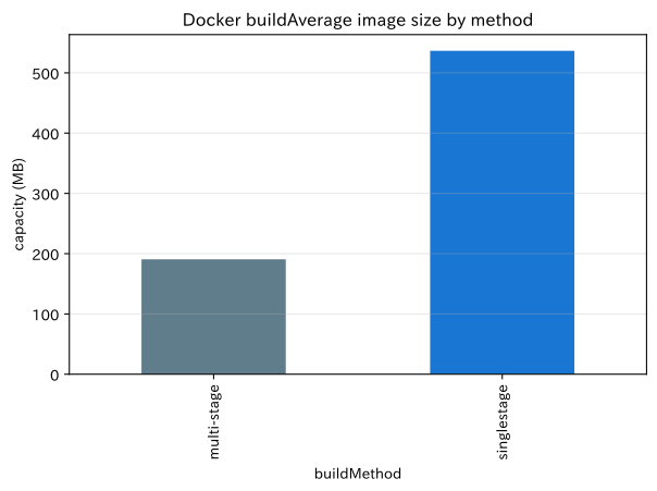
The layer cache places dependencies with minimal changes first and reuses them. Multi-stage Build does not bring build tools into the final image, reducing transfer time and the attack surface. Here, we compare capacity and time by method.

Check with Python

dockerfile = """FROM python:3.13-slim AS runtime
WORKDIR /app
COPY requirements.txt .
RUN pip install --no-cache-dir -r requirements.txt
COPY app ./app
USER 10001
CMD ["uvicorn", "app.main:app", "--host", "0.0.0.0", "--port", "8000"]
"""
summary = builds.groupby("strategy").agg(average_mb_capacity=("image_mb","mean"), average_build_seconds=("build_sec","mean")).round(1)
display(summary)
ax = summary["average_mb_capacity"].plot(kind="bar", color=["#607d8b","#1976d2"])
ax.set_title("Docker buildAverage image size by method"); ax.set_xlabel("buildMethod"); ax.set_ylabel("capacity (MB)"); ax.grid(axis="y", alpha=.3); plt.tight_layout(); plt.show()
print(dockerfile)

	average capacityMB	averagebuildseconds
strategy
multi-stage	190.6	122.1
singlestage	536.6	117.7

FROM python:3.13-slim AS runtime
WORKDIR /app
COPY requirements.txt .
RUN pip install --no-cache-dir -r requirements.txt
COPY app ./app
USER 10001
CMD ["uvicorn", "app.main:app", "--host", "0.0.0.0", "--port", "8000"]

Reading the results

Multi-stage equivalent methods have smaller capacity, reducing distribution time and vulnerability investigation targets. In practice, acceptance criteria include not only capacity but also fixed base image update frequency, SBOM, vulnerability scanning, and reproduction builds.

No.072: Containerizing the Backend

Meaning in Practice

API containers have contracts including ports, startup commands, running users, health checks, and termination signals. Not only does the process get moving, but you also need to inform the orchestrator whether requests are accepted.

Approach to Analysis and Modeling

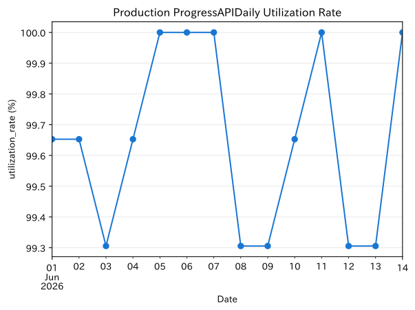
Utilization rates are measured in $A=1-\frac{T_{down}}{T_{total}}$. However, survival confirmation and readiness confirmation are separated, and communication is designed so that communication does not flow to APIs not connected to the DB.

Check with Python

availability = monitor["available"].mean()
p95 = monitor["latency_ms"].quantile(.95)
api_kpi = pd.DataFrame({"KPI":["utilization_rate","p95_response_time"],"value":[f"{availability:.3%}",f"{p95:.1f} ms"],"provisional standard":[">= 99.9%","< 250 ms"]})
display(api_kpi)
daily = monitor.set_index("time").resample("D").agg(utilization_rate=("available","mean")) * 100
ax=daily.plot(marker="o",legend=False,color="#1976d2"); ax.set_title("Production ProgressAPIDaily Utilization Rate"); ax.set_xlabel("Date"); ax.set_ylabel("utilization_rate (%)"); ax.grid(alpha=.3); plt.tight_layout(); plt.show()

	KPI	value	provisional standard
0	utilization_rate	99.653%	>= 99.9%
1	p95response time	239.5 ms	< 250 ms

Reading the results

Averaging the entire period alone hides short-term outages and peak impacts. Daily trends, p95 responses, and error rates are listed side by side, separating /live and /ready. If the standard is not met, the database wait or heavy processing is traced before adding more units.

No.073: Containerizing the Frontend

Meaning in Practice

Frontends like React can be built in Node.js, and only the generated static files can be distributed on a web server. Separating the build environment from the runtime environment prevents bringing development dependencies into production.

Approach to Analysis and Modeling

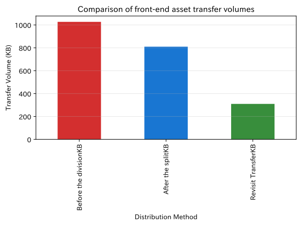
The amount of delivery affects the initial display time. Measures bundle capacity after compression, cache hit rate, Largest Contentful Paint, and more. Here, we estimate the amount transferred through asset splitting.

Check with Python

assets=pd.DataFrame({"Assets":["app.js","vendor.js","styles.css","icons"],"Before the divisionKB":[820,0,115,92],"After the splitKB":[310,360,82,58],"Revisit TransferKB":[310,0,0,0]})
display(assets)
totals=assets[["Before the divisionKB","After the splitKB","Revisit TransferKB"]].sum()
ax=totals.plot(kind="bar",color=["#d32f2f","#1976d2","#388e3c"]); ax.set_title("Comparison of front-end asset transfer volumes"); ax.set_xlabel("Distribution Method"); ax.set_ylabel("Transfer Volume (KB)"); ax.grid(axis="y",alpha=.3); plt.tight_layout(); plt.show()

	Assets	Before the divisionKB	After the splitKB	Revisit TransferKB
0	app.js	820	310	310
1	vendor.js	0	360	0
2	styles.css	115	82	0
3	icons	92	58	0

Reading the results

Splitting and long-term caching help reduce transfer volume during revisits. HTML is short, while hashed JS/CSS caches for a long time, allowing both new and old files to coexist for a certain period. We also check screen and API compatibility at the same time.

No.074: Starting a DB with Docker Compose

Meaning in Practice

Compose launches the API, screen, and database as a single configuration, enhancing the reproducibility of training and development environments. Since depends_on may only indicate the startup order, you need to check the DB’s readiness and retry on the API side.

Approach to Analysis and Modeling

Organize service dependencies as directed graphs and assign volumes only to databases that require persistence. Passwords are not fixed to the Compose body, but are passed from environment variables or secrets.

Check with Python

services=pd.DataFrame({"service":["frontend","api","db"],"Dependency":["api","db","None"],"healthcheck":["HTTP /","HTTP /ready","pg_isready"],"persistencevolume":[False,False,True],"publicport":[True,True,False]})
display(services)
checks=pd.DataFrame({"Examination":["healthcheckAvailable","DBExternal confidential","DBpersistence","fixedpasswordNone"],"Judgment":[services.healthcheck.ne("").all(),not services.loc[services.service.eq("db"),"publicport"].iloc[0],services.loc[services.service.eq("db"),"persistencevolume"].iloc[0],True]})
display(checks)

	service	Dependency	healthcheck	persistencevolume	publicport
0	frontend	api	HTTP /	False	True
1	api	db	HTTP /ready	False	True
2	db	None	pg_isready	True	False

	Examination	Judgment
0	healthcheckAvailable	True
1	DBExternal confidential	True
2	DBpersistence	True
3	fixedpasswordNone	True

Reading the results

The database is not made public, and the structure includes persistent volume and readiness confirmation. In production, instead of simply expanding Compose, we set the boundaries of responsibility for managed DB, backup, encryption, connection count, and migration.

No.075: Clarifying the differences between development environments and production environments

Meaning in Practice

In development, we prioritize speed of change and ease of investigation, while in production, we prioritize safety, availability, and traceability. On the other hand, if you separate the library version and basic configuration, the issues that occur only during the actual test increase.

Approach to Analysis and Modeling

The basic approach is to use the same image and externalize only the settings. We classify the differential items and conduct mechanical inspections to ensure that dangerous settings are not mixed into production.

Check with Python

envs=pd.DataFrame({"item":["debug","replicas","log_level","DB","TLS","automaticreload"],"Development":[True,1,"DEBUG","local container",False,True],"performance":[False,3,"INFO","managed DB",True,False],"normalization":["cannot","Configuration","Configuration","Connection only","cannot","cannot"]})
display(envs)
risk_checks={"debuginvalid":envs.loc[envs.item.eq("debug"),"performance"].iloc[0] == False,"TLSeffective":envs.loc[envs.item.eq("TLS"),"performance"].iloc[0] == True,"multiplereplica":envs.loc[envs.item.eq("replicas"),"performance"].iloc[0] >= 2}
display(pd.Series(risk_checks,name="Production Setup Inspection").to_frame())

	item	Development	performance	normalization
0	debug	True	False	cannot
1	replicas	1	3	Configuration
2	log_level	DEBUG	INFO	Configuration
3	DB	local container	managed DB	Connection only
4	TLS	False	True	cannot
5	automaticreload	True	False	cannot

	Production Setup Inspection
debuginvalid	True
TLSeffective	True
multiplereplica	True

Reading the results

While maintaining the product-specific safety settings, the app body can use the same image. Instead of branching the code heavily by environment name, it uses typed settings and startup validation, and if there are deficiencies or inconsistencies, the startup will fail.

No.076: Creating CI with GitHub Actions

Meaning in Practice

CI performs the same inspection triggered by push or pull requests, detecting basic defects before review. The important thing is not to write YAML, but to define mandatory checks, target branches, permissions, caches, and failure notifications.

Approach to Analysis and Modeling

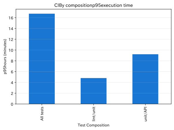
We check not only the average CI time, but also p95, failure rate, and wait times. Permissions are minimized, and external PR does not allow access to the production secret.

Check with Python

ci_summary=ci.groupby("test_level").agg(number_of_executions=("run_id","size"),average_score=("duration_min","mean"),p95_points=("duration_min",lambda x:x.quantile(.95)),defect_detection_rate=("defect_found","mean")).round(3)
display(ci_summary)
ax=ci_summary["p95_points"].plot(kind="bar",color="#1976d2"); ax.set_title("CIBy compositionp95execution time"); ax.set_xlabel("Test Composition"); ax.set_ylabel("p95hours (minutes)"); ax.grid(axis="y",alpha=.3); plt.tight_layout(); plt.show()

	number_of_executions	average_score	p95minutes	defect_detection_rate
test_level
lint/unit	42	3.169	4.806	0.119
unit/API	72	7.629	9.219	0.167
All tests	46	15.057	16.737	0.283

Reading the results

All tests have a high detection rate but also take longer to complete. In PR, high-speed inspections are mandatory, and heavy E2E is designed to be parallelized or periodically executed, improving feedback speed and detection power.

No.077: Automatically Running Tests

Meaning in Practice

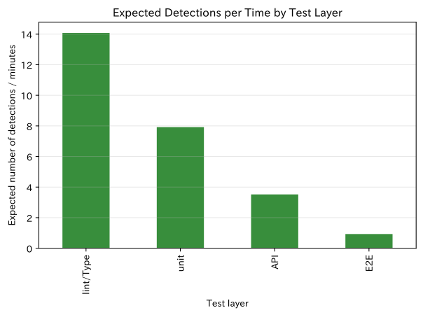
Auto-execution changes the state of “there is a test” to a state where it is checked with every change. Standalone, API, integrated, and E2E layers are combined because defects and times can be detected differ.

Approach to Analysis and Modeling

Set the expected loss as $L=\sum_i p_i c_i$ and compare the probability of defect leakage reduced by each test with the execution time. Here, we show the number of detections for 100 hypothetical defect candidates.

Check with Python

tests=pd.DataFrame({"layer":["lint/Type","unit","API","E2E"],"execution":[1.2,3.8,6.5,14.0],"candidate defect":[18,35,29,18],"detection rate":[.94,.86,.79,.72]})
tests["Expected number of detections"]=(tests["candidate defect"]*tests["detection rate"]).round(1); tests["1Minute-by-minute detection"]=(tests["Expected number of detections"]/tests["execution"]).round(2)
display(tests)
ax=tests.set_index("layer")["1Minute-by-minute detection"].plot(kind="bar",color="#388e3c"); ax.set_title("Expected Detections per Time by Test Layer"); ax.set_xlabel("Test layer"); ax.set_ylabel("Expected number of detections / minutes"); ax.grid(axis="y",alpha=.3); plt.tight_layout(); plt.show()

	layer	execution	candidate defect	detection rate	Expected number of detections	1Minute-by-minute detection
0	lint/Type	1.2	18	0.94	16.9	14.08
1	unit	3.8	35	0.86	30.1	7.92
2	API	6.5	29	0.79	22.9	3.52
3	E2E	14.0	18	0.72	13.0	0.93

Reading the results

A realistic configuration is to place high-speed static inspections and units at the entrance, protecting boundaries and key operations with API and E2E systems. Instead of reducing E2E solely through efficiency, we carefully select a few routes with significant downtime impact, such as ‘progress reflection from performance registration.‘

No.078: Deploying APIs in the Cloud

Meaning in Practice

API deployment involves not only launching images but also business changes including health checks, phased switchovers, DB migration, monitoring, and rollbacks. During production, downtime is especially managed during updates.

Approach to Analysis and Modeling

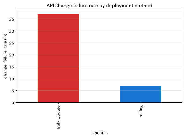
Representative KPIs are deployment frequency, change lead time, change failure rate, and recovery time. Here, we compare bulk updates and rolling updates.

Check with Python

dep=deploys[deploys.service.eq("API")].groupby("strategy").agg(number_of_times=("deploy_id","size"),average_required_score=("duration_min","mean"),change_failure_rate=("failed","mean"),average_rollback_score=("rollback_min",lambda x:x[x>0].mean())).round(2)
display(dep)
ax=(dep["change_failure_rate"]*100).plot(kind="bar",color=["#d32f2f","#1976d2"]); ax.set_title("APIChange failure rate by deployment method"); ax.set_xlabel("Updates"); ax.set_ylabel("change_failure_rate (%)"); ax.grid(axis="y",alpha=.3); plt.tight_layout(); plt.show()

	number_of_times	average_required_score	change_failure_rate	averagerollbackminutes
strategy
rolling	30	12.05	0.07	10.20
Bulk Update	19	7.63	0.37	4.61

Reading the results

Rolling updates tend to limit the impact of failures even if they take longer. However, since these are fictitious values in the teaching materials, we do not definitively determine the superiority of each method; in actual use, we check with low traffic, change the old compatible database, and set up automatic rollback conditions.

No.079: Deploying the Frontend

Meaning in Practice

You can place static assets on the CDN or similar screens, but the browser cache will retain the old version. By adding a content hash to the file name and separating the cache period between HTML and assets, you can safely switch between them.

Approach to Analysis and Modeling

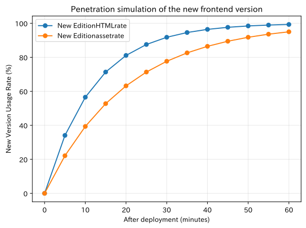
Simulate users immediately after updating using HTML update rate and asset cash hit rate. To avoid combining old HTML with deleted assets, both new and old assets are coexisting.

Check with Python

minutes=np.arange(0,61,5); rollout=pd.DataFrame({"Minutes after update":minutes}); rollout["New EditionHTMLrate"]=(1-np.exp(-minutes/12))*100; rollout["New Editionassetrate"]=(1-np.exp(-minutes/20))*100
display(rollout.iloc[[0,3,6,12]].round(1))
ax=rollout.plot(x="Minutes after update",y=["New EditionHTMLrate","New Editionassetrate"],marker="o"); ax.set_title("Penetration simulation of the new frontend version"); ax.set_xlabel("After deployment (minutes)"); ax.set_ylabel("New Version Usage Rate (%)"); ax.grid(alpha=.3); plt.tight_layout(); plt.show()

	Minutes after update	New EditionHTMLrate	New Editionassetrate
0	0	0.0	0.0
3	15	71.3	52.8
6	30	91.8	77.7
12	60	99.3	95.0

Reading the results

The penetration rates of HTML and assets do not match. It is important to maintain compatibility between old and new APIs and not to delete old assets immediately. Monitor error rates by version number, and in case of issues, revert the HTML reference destination to the previous version.

No.080: Securely managing environmental variables and secrets

Meaning in Practice

Connection destinations and log levels are separated into environment variables, while DB passwords and API keys are separated into the secret management platform. Secrets are not only stored in encrypted storage but also manage viewing permissions, hiding in logs, rotation, and even revocation.

Approach to Analysis and Modeling

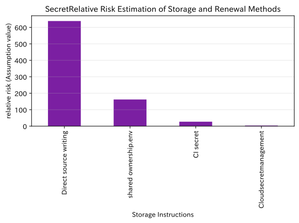
Exposure risk is simplified and placed in $R=P(expose)\times degree of influence\times Validity period$, and storage methods are compared. The figures are assumptions for prioritization purposes and are not formal risk assessments.

Check with Python

secret_risk=pd.DataFrame({"Storage Instructions":["Direct source writing","shared ownership.env","CI secret","Cloudsecretmanagement"],"Probability of exposure":[.35,.18,.06,.025],"degree of influence":[5,5,5,5],"Validity Period Date":[365,180,90,30]}); secret_risk["relative risk"]=(secret_risk["Probability of exposure"]*secret_risk["degree of influence"]*secret_risk["Validity Period Date"]).round(1)
display(secret_risk)
ax=secret_risk.set_index("Storage Instructions")["relative risk"].plot(kind="bar",color="#7b1fa2"); ax.set_title("SecretRelative Risk Estimation of Storage and Renewal Methods"); ax.set_xlabel("Storage Instructions"); ax.set_ylabel("relative risk (Assumption value)"); ax.grid(axis="y",alpha=.3); plt.tight_layout(); plt.show()

	Storage Instructions	Probability of exposure	degree of influence	Validity Period Date	relative risk
0	Direct source writing	0.350	5	365	638.8
1	shared ownership.env	0.180	5	180	162.0
2	CI secret	0.060	5	90	27.0
3	Cloudsecretmanagement	0.025	5	30	3.8

Reading the results

Centralized management and a short validity period help reduce relative risk. However, simply moving it to the management platform is not enough. Operational procedures include service unit authority, regular renewals, expiration upon retirement or outsourcing, emergency replacement in case of leaks, and log masking.

Practical Implications Seen Through Target Exercise

1. Containers are contracts of repeatability: You need to review Dockerfile, fixed versions, non-rooted execution, and healthcheck.
2. Environment differences are managed as settings, not code.: Promote the same artifact and verify production-specific safety settings at startup.
3. CI/CDmeasures both speed and stability simultaneously.: Continuously monitor not only build time but also change failure rates, recovery times, and defect leakage.
4. Deployment is a phased business change that maintains compatibility: Design with the assumption that old and new APIs, databases, and screens will temporarily coexist.
5. SecretManagement is not storage but a lifecycle.: Responsible for issuance, use, audit, renewal, relapse, and emergency replacement.

What is necessary for practical implementation

1. Definition of Business Impact: Decide on downtime allowances, busy hours, recovery objectives (RTO), data loss tolerance (RPO), and release approvers
2. Supply chain management of deliverables: Fixing dependencies, SBOM, image signing, vulnerability scanning, and establishing reliable registries.
3. Phased release: Automating development, validation, promotion to production, approval, migration, healthcheck, and rollback
4. observability: Assign version numbers and correlation IDs to logs, metrics, and traces, linking alerts to root cause investigations
5. Security Operations: Continue least privilege, secret updates, audit logs, and incident response training

Rather than aiming for a large-scale infrastructure from the start, we focus on a single critical API: “PR inspection→ image creation→ verification →environment approval→ → production monitoring→ rollback,” and improve based on measured KPIs.

Conclusion

From No.071 to No.080, to ensure the production progress API and field screens are securely delivered, we checked everything from Dockerfile to backend and front-end containerization, Compose, environment isolation, GitHub Actions, test automation, cloud deployment, and secret management.

The value lies not in adopting Docker or the cloud itself. It means reproducing the same deliverables, quickly inspecting changes, publishing limited impacts, and being able to return with justification in case of abnormalities. Since the timing and impact of downtime are critical on the manufacturing floor, technical KPIs are linked to production planning, quality, and maintenance decisions for operation.

Consultations for Corporations

At Surikoubo, we support everything from containerization of web systems and AI/APIs for manufacturing industries, CI/CD design, cloud migration, testing, monitoring, and operational KPI design to in-house training.

From the concept stage, such as “I want to systematize analysis running on the responsible person’s PC,” “I want to eliminate the dependence on individual releases,” or “I want to minimize the impact on factory operations while migrating to the cloud,” we can consult with you based on on-site constraints.

📩 Contact Us: surikobo.co.jp/contact Please feel free to consult us first.