Identifying Errors in Manufacturing KPIs: 10 Practical Basics of Floating-Point and Numerical Calculation

In manufacturing sites, sensor values, costs, yields, equipment utilization rates, and other data are aggregated by computer, and the results are used for quality judgments and investment decisions. However, the numbers on the computer are not actual numbers in mathematics. In this notebook, we will review the basics for Understanding the limits of numerical representation and preventing false judgments due to errors using a fictional precision parts factory as a subject.

This series, “100 Numerical Calculations for Manufacturing Decision-Making,” covers 100 questions that teach step-by-step learning from floating-point numbers to equations, linear algebra, interpolation, calculus, differential equations, and optimization, all linked to real-world decision-making. The first installment covers the foundations No.001 to No.010.

[!NOTE] This material is a notebook previously used by Surikoubo (or personally by the representative, Kazuyama), and has been reconstructed, edited, and published with the company’s permission.
All data listed is fictional and has no relation whatsoever to real companies, factories, or figures.

1. Introduction: Practical Challenges in Manufacturing Covered in This Article

In precision parts factories, both large and small figures are handled simultaneously, such as dimensional tolerances in the few micrometers, material usage in the millions of pieces, and equipment logs in the second. The issue in this article is that even if the formula is theoretically correct, the sum value can shift due to numerical representation and order of operations, which can change the judgment of pass/fail, abnormality, and profitability.

2. Common Situations on Site

• Display digits and data types differ between Excel, PLC, database, and Python
• Even simple calculations like 0.1 + 0.2 do not match expectations when the internal values
• Even if you make a tiny adjustment to the huge cumulative value, it won’t be reflected
• When the difference between close measurements is taken, the significant digit is lost.
• Mistakenly thinking that just because the correct value is large is a big error

3. Why is this issue difficult to judge?

Since the screen displays the results in a rounded form, internal errors are hard to see, whereas in threshold determination, even slight differences can change the conclusion. Also, whether to look at absolute error or relative error depends on the intended use. In quality assurance, it is necessary to design calculation methods and judgment rules, including units, resolution, and tolerances.

4. The overall picture of exercise covered this time

No.	Theme	Key Issues in Manufacturing
001	What is numerical calculation?	The Relationship Between Theoretical Values, Approximate Values, and Decision-Making
002	floating-point representation	Difference between display values and internal values
003	IEEE 754	Data types, signs, exponents, mantissa
004	rounding error	How to round the amounts and aggregation
005	Drop in the digits	Differences in Nearby Measurements
006	Information Leakage	Micro-addition to large cumulative values
007	overflow	Divergence of indicators and model calculations
008	Underflow	Loss of Minute Probability
009	Machine Epsilon	Minimum difference identifiable by computer
010	Evaluation of numerical errors	Absolute error, relative error, and acceptable criteria

5. Preparing the Python environment

It does not rely on external data and reproduces using NumPy, pandas, and matplotlib. Random seed is fixed so that the same result is achieved.

import sys
import numpy as np
import pandas as pd
import matplotlib
import matplotlib.pyplot as plt
import japanize_matplotlib

SEED = 42
rng = np.random.default_rng(SEED)
pd.set_option("display.precision", 10)

print(f"Python     : {sys.version.split()[0]}")
print(f"NumPy      : {np.__version__}")
print(f"pandas     : {pd.__version__}")
print(f"matplotlib : {matplotlib.__version__}")

Python     : 3.13.1
NumPy      : 2.5.1
pandas     : 3.0.3
matplotlib : 3.11.0

6. Creation of Fictional Data

This assumes measuring 1,000 shafts with a nominal dimension of 50,000 mm and a tolerance of ±0.010 mm. The measuring instrument displays a resolution of 0.001 mm and holds both the internal value close to the true value and the displayed value. Additionally, quantities and unit prices are created for cost aggregation.

n = 1_000
measurement_raw = 50.0 + rng.normal(0, 0.004, n)
measurement_display = np.round(measurement_raw, 3)
factory_df = pd.DataFrame({
    "lot": np.repeat(["L-A", "L-B", "L-C", "L-D"], n // 4),
    "measurement_raw_mm": measurement_raw,
    "measurement_display_mm": measurement_display,
    "quantity": rng.integers(80, 151, n),
    "unit_cost_yen": rng.uniform(118.0, 123.0, n),
})
factory_df.head()

	lot	measurement_raw_mm	measurement_display_mm	quantity	unit_cost_yen
0	L-A	50.0012188683	50.001	93	120.4056155088
1	L-A	49.9958400636	49.996	125	121.9110559763
2	L-A	50.0030018048	50.003	108	121.7399506448
3	L-A	50.0037622589	50.004	104	122.0753654811
4	L-A	49.9921958592	49.992	129	120.2412031659

7. No.001: What is Numerical Computation?

Meaning in Practice

Numerical computation is not just about looking at analytical formulas, but also about finding approximate values from a finite number of digits and converting them into shapes usable for on-site decision-making. For example, the average dimension is determined by dividing the total of all measured values by the number of pieces, but quality assessment cannot be achieved unless you determine the data type, missing processing, rounding, and tolerances.

Approach to Analysis and Modeling

If the measurement is $x_1,\ldots,x_n$, then the average is

$$\bar{x}=\frac{1}{n}\sum_{i=1}^{n}x_i$$

That’s right. In numerical calculations, input errors, algorithm approximation errors, and finite precision rounding errors are propagated to the results. The goal is not to “perfectly reproduce the true value,” but to ensure the accuracy necessary for decision-making.

Check with Python

summary_001 = factory_df["measurement_raw_mm"].agg(["count", "mean", "std", "min", "max"])
summary_001.to_frame("Measurement value (mm)")

	Measurement value (mm)
count	1000.0000000000
mean	49.9998844338
std	0.0039568684
min	49.9854063487
max	50.0127154147

Reading the results

By listing not only the mean but also the standard deviation and range, you can distinguish between process centers and variance. It is important that numerical results are not just isolated numbers, but managed together with units, calculation conditions, and determination objectives.

8. No.002: Floating-Point Representation

Meaning in Practice

Many decimals are binary and cannot be represented as finite digits. Therefore, when adding costs or comparing them to thresholds, even if the displayed value is the same, the internal values may differ slightly.

Approach to Analysis and Modeling

Floating-point numbers are conceptually defined using sign $s$, mantissa $m$, base $\beta$, and exponent $e$

$x=(-1)^s\times m\times\beta^e$

This is how it is expressed. Python’s usual float is double the accuracy of base 2. For precise decimal calculation of amounts, integers (such as sen) and decimal.Decimal are also options.

Check with Python

from decimal import Decimal

floating = 0.1 + 0.2
exact_decimal = Decimal("0.1") + Decimal("0.2")
pd.DataFrame({
    "Calculation method": ["binary64 float", "Decimal(Generated from a string)"],
    "Results": [format(floating, ".17f"), str(exact_decimal)],
    "0.3Matches": [floating == 0.3, exact_decimal == Decimal("0.3")],
})

	Calculation method	Results	0.3Matches
0	binary64 float	0.30000000000000004	False
1	Decimal(Generated from a string)	0.3	True

Reading the results

float results are close to 0.3, but they don’t exactly match. For sensor processing, you select expressions that fit your purpose, such as comparison with tolerance, and for accounting, decimal or integer for the smallest currency unit.

9. No.003：IEEE 754

Meaning in Practice

When float32 and float64 coexist among instruments, databases, and analytical platforms, not only storage capacity but also significant bits and calculation results change. You need to specify the data type in the interface specification.

Approach to Analysis and Modeling

In IEEE 754’s representative binary format, float32 is 1 sign bit, 8 exponential bits, and 23 mantiss bits, and float64 is 1, 11, and 52. Since the normalizer has an implicit first 1, the effective accuracy is equivalent to 24 bits and 53 bits, respectively.

Check with Python

rows = []
for dtype in [np.float32, np.float64]:
    info = np.finfo(dtype)
    rows.append({
        "type": dtype.__name__, "bytes": info.bits // 8,
        "10Reference for Base Significant Figures": info.precision,
        "maximum value": info.max, "Minimal normalized positive number": info.tiny,
    })
pd.DataFrame(rows)

	type	bytes	10Reference for Base Significant Figures	maximum value	Minimal normalized positive number
0	float32	4	6	3.4028234664e+38	1.1754943508e-38
1	float64	8	15	1.7976931349e+308	2.2250738585e-308

Reading the results

float32 is memory-efficient but generally achieves about 7 digits of accuracy. Long-term cumulative values and high-precision measurements may fall short. Based on the required accuracy, data volume, and computation speed, the type is determined and the conversion points are tested.

10. No.004: Rounding Error

Meaning in Practice

The result differs depending on whether you round the cost of each part into 1 yen increments and then add it up, or if you round it after the total. The rules for quotation, standard cost, and billing should be unified down to the calculation order.

Approach to Analysis and Modeling

If we set the rounding operation to $\operatorname{fl}(x)$, then generally,

$\sum_i \operatorname{fl}(x_i) \ne \operatorname{fl}\left(\sum_i x_i\right)$

That’s right. Additionally, we distinguish between approximate errors in binary floating-point representations and the use of decimal rounding as a business rule.

Check with Python

line_cost = factory_df["quantity"] * factory_df["unit_cost_yen"]
rounding_comparison = pd.Series({
    "by itemized item1After rounding, total": np.round(line_cost, 0).sum(),
    "After adding the total without rounding,1rounded": np.round(line_cost.sum(), 0),
})
rounding_comparison.to_frame("Total cost (yen)").assign(
    difference_from_the_standard=lambda x: x["Total cost (yen)"] - x.iloc[1, 0]
)

	Total cost (yen)	difference_from_the_standard
by itemized item1After rounding, total	13856809.0	13.0
After adding the total without rounding,1rounded	13856796.0	0.0

Reading the results

The difference is not necessarily a misimplementation, but rather a difference in the rounded terms. However, for bulk invoices, the differences accumulate. Specify the “rounded units, methods, and timing” in the requirements definition, and prepare examples of reconciliation with the accounting system.

11. No.005: Down from the Digits

Meaning in Practice

If you take a large and nearly close difference between two values, the common upper digits are canceled out, leaving only the lower digits with relatively larger errors. Be careful with slight displacements from reference positions and differences in energy balance.

Approach to Analysis and Modeling

When $a$ and $b$ are close, the valid digits of $a-b$ are fewer than the valid digits of the input. Countermeasures include deformation into stable formulas, centering to draw reference values early, and using high-precision models.

Check with Python

reference64 = np.float64(100_000_000.0)
measured64 = np.float64(100_000_000.125)
reference32, measured32 = np.float32(reference64), np.float32(measured64)

pd.DataFrame({
    "type": ["float64", "float32"],
    "reference value": [reference64, reference32],
    "Measurement value": [measured64, measured32],
    "difference": [measured64-reference64, measured32-reference32],
})

	type	reference value	Measurement value	difference
0	float64	100000000.0	100000000.125	0.125
1	float32	100000000.0	100000000.000	0.000

Reading the results

In float32, the difference of 0.125 disappeared. Rather than storing coordinates as huge values from the origin, it is effective to preserve effective digits during the data design phase, such as storing them as displacements from equipment standards.

12. No.006: Information Drop

Meaning in Practice

If you add a very small value to a large cumulative value, the small value will fall below the representable digit and will not be reflected in the addition result. This occurs when accumulating small increments from high-speed sensors over a long period.

Approach to Analysis and Modeling

The interval between floating-point numbers expands along with the absolute value of the value. If the small $\delta$ for the large value $A$ is smaller than the representation interval near the $A$, it becomes $\operatorname{fl}(A+\delta)=A$. Methods such as summing from smaller values and compensated sums are effective strategies.

Check with Python

values = np.concatenate(([1e16], np.ones(1_000_000)))
naive_sum = values.sum()
small_first_sum = values[::-1].sum()
import math
compensated_sum = math.fsum(values.tolist())

pd.DataFrame({
    "Methods": ["From the large priceNumPyTotal", "From low pricesNumPyTotal", "math.fsum(Total compensation)"],
    "Total": [naive_sum, small_first_sum, compensated_sum],
    "Difference from theoretical values": [naive_sum-(1e16+1e6), small_first_sum-(1e16+1e6), compensated_sum-(1e16+1e6)],
})

	Methods	Total	Difference from theoretical values
0	From the large priceNumPyTotal	1.0000000001e+16	-12.0
1	From low pricesNumPyTotal	1.0000000001e+16	0.0
2	math.fsum(Total compensation)	1.0000000001e+16	0.0

Reading the results

Even if the values are the same, the result will change depending on the order of addition. For key cumulative KPIs, units are properly scaled, stable aggregation methods are adopted, and tolerances for recounting are defined.

13. No.007: Overflow

Meaning in Practice

Failure models including exponential functions, likelihood calculations, and incorrect unit conversion indicators can exceed the maximum value of the type and become inf. It also contaminates subsequent averages and optimization results.

Approach to Analysis and Modeling

The maximum finite value of float64 is about $1.8 imes10^{308}$. In exponential calculation, methods such as calculating in the logarithmic area rather than direct multiplication, verifying input ranges, and detecting anomalies with isfinite are effective.

Check with Python

growth_rates = np.array([700.0, 710.0, 720.0])
with np.errstate(over="ignore"):
    direct = np.exp(growth_rates)
result_007 = pd.DataFrame({"index": growth_rates, "exp(x)": direct, "Finite value?": np.isfinite(direct)})
result_007

	index	exp(x)	Finite value?
0	700.0	1.0142320547e+304	True
1	710.0	inf	False
2	720.0	inf	False

Reading the results

Simply removing warnings is not enough to address the issue. Verify input limits, units, and finiteness, and treat products or exponents as logarithmic values if you only compare them. Avoid quietly excluding inf as a loss-making value.

14. No.008: Underflow

Meaning in Practice

When multiplied by many small defect probabilities and likelihoods, even if the true value is positive, the calculation result becomes zero. This is why anomaly detection models cannot compare candidates between candidates.

Approach to Analysis and Modeling

The product of probabilities $P=\prod_i p_i$ can be obtained using logarithms,

$\log P=\sum_i \log p_i$

That’s how it works. By converting the product to sum, it is less likely to exceed the expressible range and allows for maintenance of large and small comparisons.

Check with Python

probabilities = np.full(1_000, 0.01)
direct_probability = np.prod(probabilities)
log_probability = np.log(probabilities).sum()
pd.Series({
    "direct product of probability": direct_probability,
    "logarithmic probability": log_probability,
    "Held as a finite logarithm": np.isfinite(log_probability),
}).to_frame("value")

	value
direct product of probability	0.0
logarithmic probability	-4605.1701859881
Held as a finite logarithm	True

Reading the results

The direct product becomes zero, but the logarithmic probability can still be retained. In predictive maintenance and quality models, log-likelihood is used as the standard, distinguishing whether “0” is true zero or a numerical limit.

15. No.009: Mechanical Epsilon

Meaning in Practice

Machine Epsilon is a relative interval that the calculator can distinguish within a 1.0 approximity. However, you can’t use the machine epsilon as a margin for every comparison.

Approach to Analysis and Modeling

Mechanical Epsilon $\varepsilon$ is the smallest positive number of the target type that is $1+\varepsilon>1$. The actual interval near value $x$ can be checked in np.spacing(x). Operational tolerances are set with priority on measurement resolution and tolerances.

Check with Python

scale_values = np.array([1.0, 50.0, 1e8, 1e16])
pd.DataFrame({
    "value x": scale_values,
    "xThe interval to the next expression value in the neighborhood": np.spacing(scale_values),
    "relative interval": np.spacing(scale_values) / scale_values,
}).assign(float64_machine_epsilon=np.finfo(np.float64).eps)

	value x	xThe interval to the next expression value in the neighborhood	relative interval	float64Machine Epsilon
0	1.0000000000e+00	2.2204460493e-16	2.2204460493e-16	2.2204460493e-16
1	5.0000000000e+01	7.1054273576e-15	1.4210854715e-16	2.2204460493e-16
2	1.0000000000e+08	1.4901161194e-08	1.4901161194e-16	2.2204460493e-16
3	1.0000000000e+16	2.0000000000e+00	2.0000000000e-16	2.2204460493e-16

Reading the results

The absolute spacing widens as the value increases. For comparison, it is important to set relative and absolute tolerances for np.isclose according to the application, and not to confuse machine accuracy with process capability.

16. No.010: Evaluation of Numerical Errors

Meaning in Practice

The evaluation changes depending on whether the error is viewed only by “how many millimeters of error is off” or “how much is it deviated from the standard.” For quality, cost, and simulation verification, indicators and passing criteria that match the objectives are necessary.

Approach to Analysis and Modeling

For true value $x$ and approximate value $\hat{x}$, the absolute error and relative error are

E_{\mathrm{rel}}=\frac{|\hat{x}-x|}{|x|}$$ That's right. If the true value is near zero, the relative error becomes unstable, so use the absolute tolerance. If there is uncertainty in the reference value itself, that uncertainty is included in the evaluation. ### Check with Python ```python raw = factory_df["measurement_raw_mm"].to_numpy() displayed = factory_df["measurement_display_mm"].to_numpy() abs_error = np.abs(displayed - raw) rel_error = abs_error / np.abs(raw) error_summary = pd.Series({ "maximum_absolute_error (mm)": abs_error.max(), "mean absolute error (mm)": abs_error.mean(), "Maximum relative error (%)": 100 * rel_error.max(), "Half the display resolution (mm)": 0.0005, }) display(error_summary.to_frame("value")) fig, ax = plt.subplots(figsize=(8, 4.5)) ax.hist(abs_error * 1_000, bins=20, color="#2878B5", edgecolor="white") ax.axvline(0.5, color="#C82423", linestyle="--", label="Half the display resolution") ax.set_title("Measured values0.001 mmRounding error when displayed in units") ax.set_xlabel("absolute_error (µm)") ax.set_ylabel("Measurement Quantity") ax.grid(True, alpha=0.3) ax.legend() plt.tight_layout() plt.show() ``` <style scoped> .dataframe tbody tr th:only-of-type { vertical-align: middle; } .dataframe tbody tr th { vertical-align: top; } .dataframe thead th { text-align: right; } </style> <table border="1" class="dataframe"> <thead> <tr style="text-align: right;"> <th></th> <th>value</th> </tr> </thead> <tbody> <tr> <th>maximum_absolute_error (mm)</th> <td>0.0004999639</td> </tr> <tr> <th>mean absolute error (mm)</th> <td>0.0002556658</td> </tr> <tr> <th>Maximum relative error (%)</th> <td>0.0009999378</td> </tr> <tr> <th>Half the display resolution (mm)</th> <td>0.0005000000</td> </tr> </tbody> </table> /var/folders/3y/fmw40k0x78xblvb3gkcyvy1h0000gn/T/ipykernel_76425/1972374313.py:22: UserWarning: Glyph 181 (\N{MICRO SIGN}) missing from font(s) IPAexGothic. plt.tight_layout() /Users/hiroshi/private/kobo/notebook/.venv/lib/python3.13/site-packages/IPython/core/pylabtools.py:170: UserWarning: Glyph 181 (\N{MICRO SIGN}) missing from font(s) IPAexGothic. fig.canvas.print_figure(bytes_io, **kw) 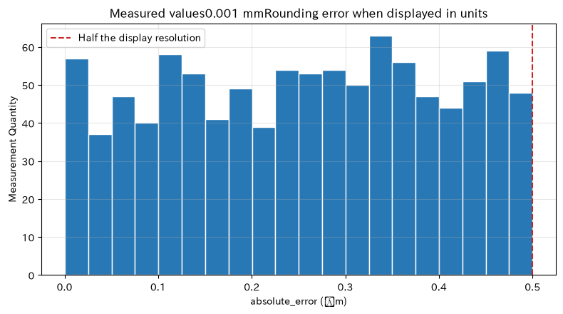 ### Reading the results The absolute error from rounding is, in theory, less than half the display increment of 0.001 mm. The operational requirements determine whether this error is sufficiently small for a tolerance ± 0.010 mm, or whether products near the judgment boundary should be remeasured. Even if the relative error is small, if you cross the pass/fail boundary, you can't ignore it. ## 17. Practical Insights Seen Through Target Exercise 1. **Data types are design items**: Determined not only by storage capacity but also by measurement resolution, cumulative period, and calculation content. 2. **The rounded rules are for business purposes.**: Standardize not only the number of digits but also the method and timing. 3. **The correctness of the formula and the stability of the calculation are different**: Even if mathematically equivalent, the results differ with finite precision. 4. **Do not mechanically exclude outliers**: Check whether `inf`, 0, and `NaN` indicate numerical limits. 5. **Connecting errors to judgment criteria**: Absolute and relative errors, measurement uncertainty, tolerances, and losses are evaluated together. ## 18. What is necessary for practical implementation - Inventory data types and units among PLCs, sensors, databases, and BIs - Define specifications for accuracy, rounding, defects, finiteness, and tolerance for each key KPI - Prepare automated tests including boundary values, large and small values, and addition order - Record source data, conversion history, library versions, and random seed numbers to ensure reproducibility. - Quality assurance, accounting, production technology, and IT are all confirmed to be accepted using the same calculation example If you want to start small, it's realistic to select three KPIs directly related to pass/fail, billing, and equipment downtime, and visualize the current calculation path and error budget. ## 19. Summary Floating-point numbers are convenient but represent finite expressions. By understanding rounding errors, digit drops, information drops, overflow, and underflow, and distinguishing between machine epsilon and operational tolerances, calculation results can be safely used for decision-making. What matters is not just increasing the number of digits, but designing data representation, stable computation, and verification criteria as a unified whole. ## 20. Consultations for Corporations At Surikoubo, we offer consultations not only on manufacturing data analysis, numerical simulation, mathematical optimization, and AI implementation, but also on reviewing the calculation accuracy of existing KPIs and conducting in-house training. We organize the characteristics of field data and decision-making flows, supporting everything from PoC to operational design. > 📩 **Contact Us**: [surikobo.co.jp/contact](https://surikobo.co.jp/contact) > Please feel free to consult us first.